Seismic Vulnerability Assessment of a Shallow Two-Story Underground RC Box Structure

Abstract

Tunnels, culverts, and subway stations are the main parts of an integrated infrastructure system. Most of them are constructed by the cut-and-cover method at shallow depths (mainly lower than 30 m) of soil deposits, where large-scale seismic ground deformation can occur with lower stiffness and strength of the soil. Therefore, the transverse racking deformation (one of the major seismic ground deformation) due to soil shear deformations should be included in the seismic design of underground structures using cost- and time-efficient methods that can achieve robustness of design and are easily understood by engineers. This paper aims to develop a simplified but comprehensive approach relating to vulnerability assessment in the form of fragility curves on a shallow two-story reinforced concrete underground box structure constructed in a highly-weathered soil. In addition, a comparison of the results of earthquakes per peak ground acceleration (PGA) is conducted to determine the effective and appropriate number for cost- and time-benefit analysis. The ground response acceleration method for buried structures (GRAMBS) is used to analyze the behavior of the structure subjected to transverse seismic loading under quasi-static conditions. Furthermore, the damage states that indicate the exceedance level of the structural strength capacity are described by the results of nonlinear static analyses (or so-called pushover analyses). The Latin hypercube sampling technique is employed to consider the uncertainties associated with the material properties and concrete cover owing to the variation in construction conditions. Finally, a large number of artificial ground shakings satisfying the design spectrum are generated in order to develop the seismic fragility curves based on the defined damage states. It is worth noting that the number of ground motions per PGA, which is equal to or larger than 20, is a reasonable value to perform a structural analysis that produces satisfactory fragility curves.

1. Introduction

In previous design specifications for underground structures in Japan, the seismic design is not usually considered in the transverse direction because there has been a strong belief that underground structures are stable following the deformation of the surrounding soil during an earthquake. Consequently, the Daikai subway system as well as tunnels and metro stations where the design did not consider the earthquake load [1] were hit by the Hyogoken-Nanbu earthquake of magnitude 7.2 based on Japan Meteorological Agency scale (roughly equivalent to a moment magnitude M_w of 6.9) in 1995 [2]. The general damage pattern showed the lack of load carrying capacity against shear at the center columns that led to the collapse of the tunnel ceiling slabs [1,3]. Moreover, many of infrastructures worldwide have also experienced significant damages in recent earthquakes such as in the M_w 7.7 Chi-Chi Taiwan in 1999 [4], M_w 6.3 Baladeh in 2004 [5], and M_w 7.0 Haiti in 2010 [6]. Several design hypotheses for the analysis applying seismic loadings are suggested. However, the real seismic behavior during shaking remains unaddressed [7]. There are many methods used to perform the soil–structure interaction (SSI). Whereas the sophisticated model using full dynamic numerical analysis is expected to provide accurate results at high computational cost, other methods such as pseudo-static or equivalent static solutions are also acceptable for practical purposes despite a low accuracy in calculation. The static seismic analysis method, so-called the ground response acceleration method for buried structures (GRAMBS) has proven its effectiveness in modeling the dynamic response behavior considering the SSI [8,9]. The method was first proposed by Katayama in 1990 [8], where the calculated accelerations were converted into static force and applied to the finite element method (FEM) model which assigning horizontal rollers at both sides and a fixed base condition. The analytical method had been verified to be effective by comparing its results with those of the dynamic analysis using FLUSH-VB [8]. From the experiment in Katayama’s research, the required computing time for GRAMBS was only one-tenth of that for the analysis using FLUSH-VB, with relatively identical results. In addition, other recent quasi-static methods also show satisfactory results similar to GRAMBS. Particularly, Akira Tateishi proposed a new method called the ground response method (GRM) in 2005 [9] by studying a seismic load for the seismic deformation method based on the dynamic substructure method. Then, those seismic stresses and seismic deformation of the ground were verified to be applied to underground structure. The GRM uses the inertia forces calculated from response accelerations of a free field as the main seismic load similar to GRAMBS, and the difference is that the outer boundary conditions are replaced with equivalent nodal forces that reproduce seismic strains of a free field to a near field. The GRM results had proven the accuracy of Katayama’s method. Out of the GRAMBS’s benefits such as time efficiency and its simplicity, its main shortcoming is not applicable to an inclined input of a shear wave and a longitudinal wave because of the constraints of displacements at the boundaries [9]. Even though GRAMBS has been developed for a long time, it is still the most effective and reliable static seismic analysis method because it was verified with various dynamic finite element analyses [10,11,12], especially the validity of GRAMBS was confirmed from the result of a small-scale model of tunnel embedded in a shear soil column on shaking table conducted by Tohma et al. [13]. Therefore, GRAMBS is trusted to be a tool for structural analysis in this study.

Most of the structures in the form of tunnels or parking lots have at least two levels, which allow functional arrangements for ticket machines, platforms, ATM, passenger access, ventilation, equipment, and staff rooms. Therefore, a typical two-story reinforced concrete underground box structure is considered as the main subject of this research. The objective is to propose a comprehensive numerical approach for the development of fragility curves. In addition, the number (10, 20, 30, 40, and 50) of earthquakes per peak ground acceleration (PGA) is investigated in order to determine the effective number, which is appropriate in a practical analysis.

2. Analytical Procedure for Constructing Fragility Curves

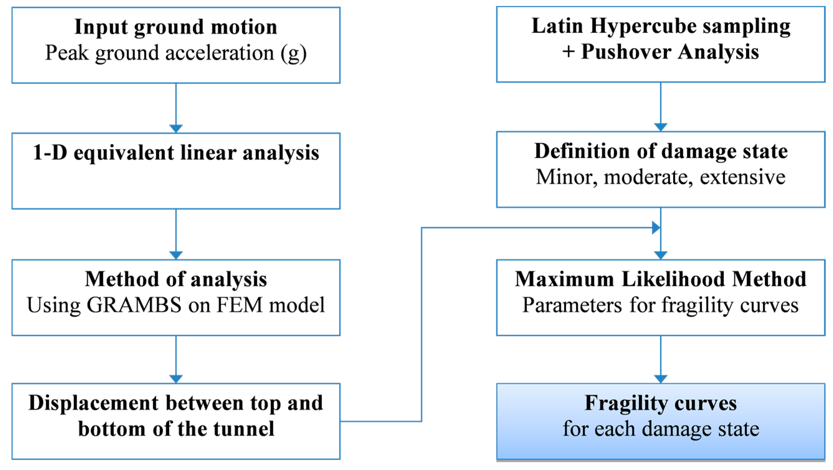
As mentioned above, the objective of this study is to develop a comprehensive numerical approach for the construction of fragility curves focusing on a shallow two-story reinforced concrete underground box structure in a highly-weathered soil. The frame work of the study is divided into many subtasks as shown in Figure 1. The numerical approach is based on the GRAMBS method for analyzing the subway station structure instead of applying the dynamic time-history analysis because it significantly improves the efficiency by reducing the computational cost without sacrificing the accuracy. A large set of input artificial ground motions representing different levels of earthquake intensity are generated. The responses of the free-field ground shaking are calculated through a 1D equivalent linear analysis for an increasing level of earthquake intensity. Then, the accelerations at the time of the maximum displacement between top and bottom of the tunnel are obtained. All the accelerations along the soil depth are converted into static force and applied to the structure. On the other hand, the damage states that indicate the exceedance level of the structural strength capacity are described by the pushover analysis considering the uncertainties on the material properties and concrete cover. For this purpose, the Latin hypercube sampling method is used to generate a set of random variables. Finally, the fragility curves are constructed based on the development of a damage index (DI) with the increase of seismic intensity. The fragility curve parameters are estimated by applying the maximum likelihood estimate (MLE).

2.1. Structural Analysis Using GRAMBS

In a soil-structure system, the major external forces on the structure are provided by the effective dynamic response of the surrounding soil. The dynamic problem of such a buried structure certainly becomes the quasi-static soil-structure interaction problem of the system. When a two-dimensional system is excited by the horizontal input ground motion, ${\ddot{\mathrm{X}}}_{\mathrm{g}}\left(\mathrm{t}\right)$, the equation of motion [8] is

$$\left[\mathrm{M}\right]\{\ddot{\mathrm{X}}\left(\mathrm{t}\right)\}+\left[\mathrm{C}\right]\{\dot{\mathrm{X}}\left(\mathrm{t}\right)\}+\left[\mathrm{K}\right]\left\{\mathrm{X}\left(\mathrm{t}\right)\right\}=-\left[\mathrm{M}\right]\left\{\mathsf{\iota }\right\}{\ddot{\mathrm{X}}}_{\mathrm{g}}\left(\mathrm{t}\right),$$

(1)

where [M], [C], and [K] are the mass matrix, damping matrix, and stiffness matrix, respectively. X(t) is the relative displacement vector. $\left\{\mathsf{\iota }\right\}$ is the influence vector which represents the relationship between seismic input direction and analytical model degree-of-freedom (DOF). At first, the tunnel structure is neglected, and the system is assumed to consist only of the soil layer. The problem therefore turns out to be a free-field response of a uniform soil. The stress of a small portion of soil from the depth j to j + 1 can be expressed as [8]

$${\mathsf{\sigma }}^{\mathrm{j}}=\left[\mathrm{D}\right]\left[\mathrm{B}\right]{\mathrm{u}}^{\mathrm{j}},$$

(2)

where σ^j represents the stress of the soil from the depth j to j + 1, [D] is the material property matrix, related to Young’s modulus and Poisson’s ratio, [B] is the strain-displacement matrix which indicates the relationship between relative displacement and shear strain, and u^j is the relative displacement between the depth j and j + 1. Taking the time, t_m, when the portion of the soil to be replaced by the tunnel shows the maximum relative displacement between the top and bottom levels of the tunnel, Equation (2) must be maximized and should also satisfy Equation (1) as

$${\mathrm{X}}^{\mathrm{j}}\left({\mathrm{t}}_{\mathrm{m}}\right){=\mathrm{X}}^{\mathrm{j}+1}\left({\mathrm{t}}_{\mathrm{m}}\right){+\mathrm{u}}^{\mathrm{j}},$$

(3)

Rewriting Equation (1), we obtain

$$\left[\mathrm{K}\right]\left\{\mathrm{X}\left({\mathrm{t}}_{\mathrm{m}}\right)\right\}=-\left[\mathrm{M}\right](\{\ddot{\mathrm{X}}\left({\mathrm{t}}_{\mathrm{m}}\right)\}+\left\{\mathsf{\iota }\right\}{\ddot{\mathrm{X}}}_{\mathrm{g}}\left({\mathrm{t}}_{\mathrm{m}}\right))-\left[\mathrm{C}\right]\{\dot{\mathrm{X}}\left({\mathrm{t}}_{\mathrm{m}}\right)\},$$

(4)

where the right-hand side of Equation (4) is the dynamic force applied on the full depth of the soil column at time t_m. Because the time is fixed, it becomes a solution to the static problem. If the damping of the soil is small, Equation (4) can be approximated as [8]

$$\left[\mathrm{K}\right]\left\{\mathrm{X}\left({\mathrm{t}}_{\mathrm{m}}\right)\right\}=-\left[\mathrm{M}\right](\{\ddot{\mathrm{X}}\left({\mathrm{t}}_{\mathrm{m}}\right)\}+\left\{\mathsf{\iota }\right\}{\ddot{\mathrm{X}}}_{\mathrm{g}}\left({\mathrm{t}}_{\mathrm{m}}\right)),$$

(5)

If the portion of the soil is replaced by the tunnel, then the corresponding parts of the matrices [M], [K], [D], and [B] relating to the calculation of the maximum stress described earlier are replaced by those of the tunnel. In addition, u^j becomes equivalent to the maximum relative displacement between the top and bottom levels of the tunnel. Finally, the maximum stress state of the tunnel surrounded by the soil is predicted.

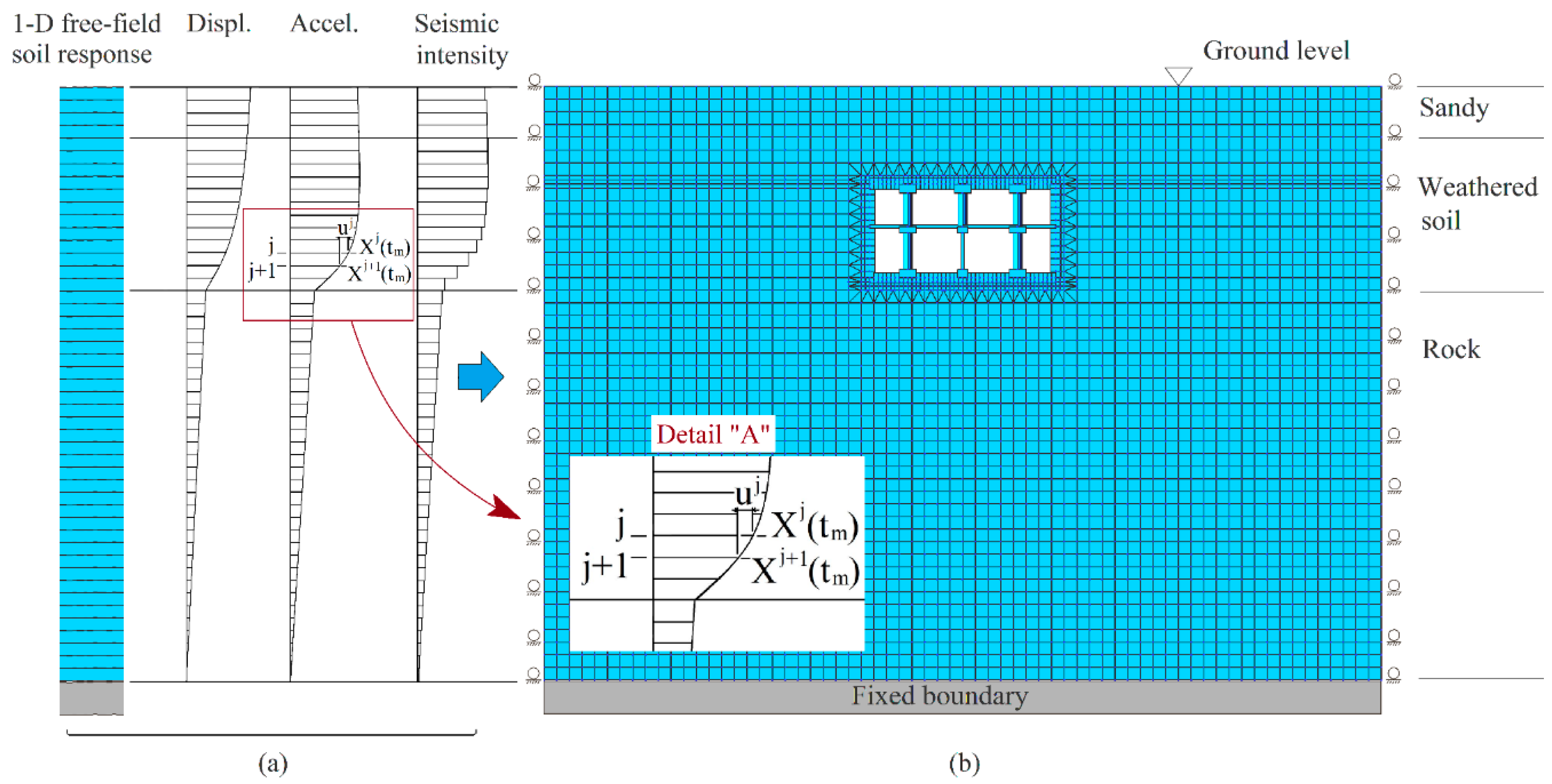
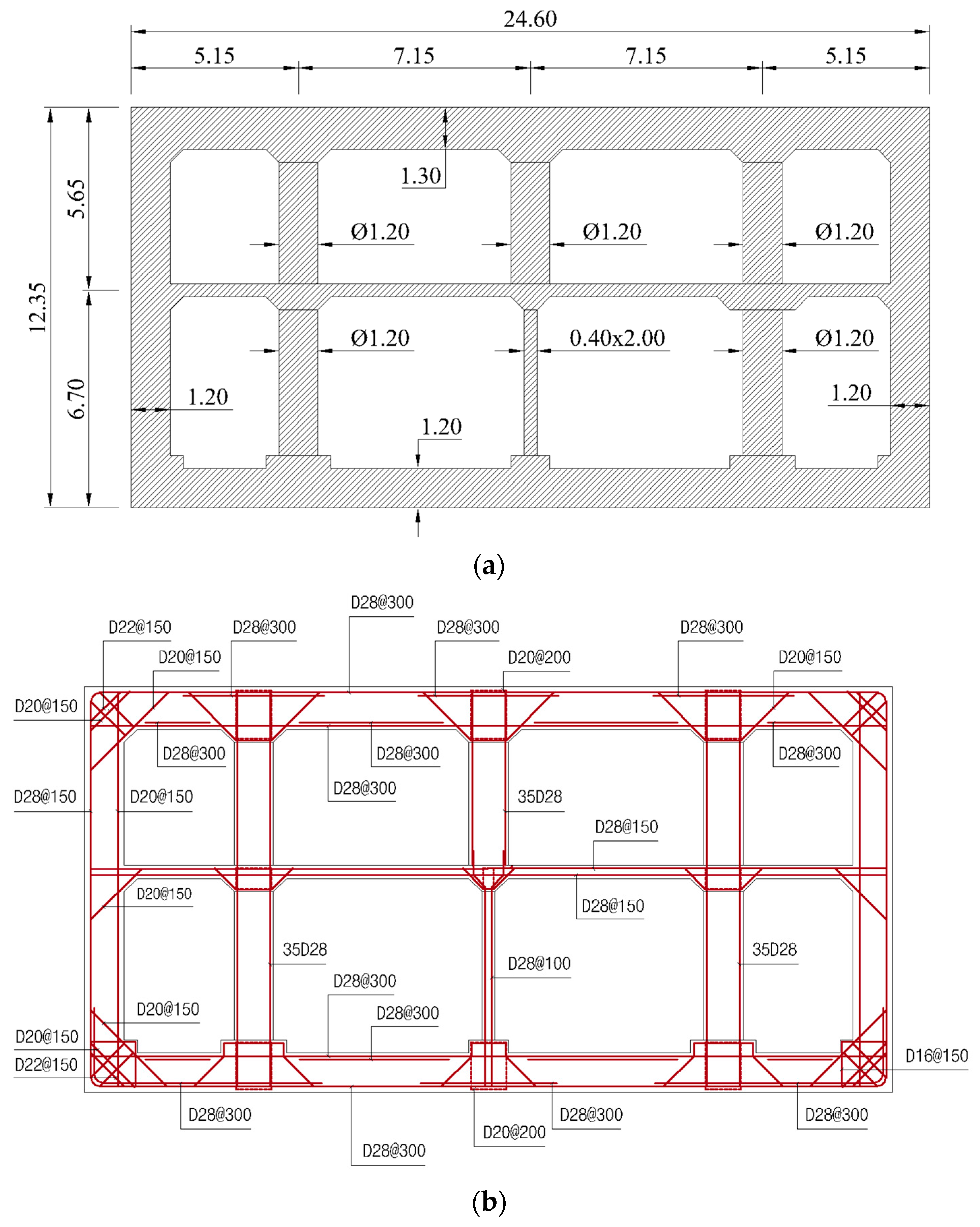
In this study, at first, without considering the subway station structure, the free-field soil response analysis for each sub-layer is performed using the 1D equivalent linear method [14]. The aim is mainly to obtain the time-dependent displacement and acceleration responses of each layer. The ground response acceleration at time t_m is considered for the whole depth of the soil column and converted into a body force as illustrated in Figure 2a. Then, it is applied to every node of a 2D finite element model for the static analysis. A numerical example has been solved, in which a two-story reinforced concrete subway station and near field of the adjacent ground are modeled using the MIDAS finite element program [15]. The subway station base is placed on a rocky layer at 22.6 m depth with a buried soil cover of approximately 10.25 m high. Boundary conditions of the ground model comprise a fixed base and roller supports at both sides which fix vertical direction and free to rotate and translate in horizontal direction when the ground subjected by horizontal shaking as shown in Figure 2b. The soil layers and their physical properties are summarized in

Table 1. Physical properties of soil.

Soil Layer	Unit	Sandy	Weathered Soil	Rock
Mass density	kg/m3	1800	2000	2300
Shear wave velocity	m/s	275	500	1500
Poisson’s ratio	-	0.35	0.35	0.25
Thickness	m	6.0	16.6	-

.

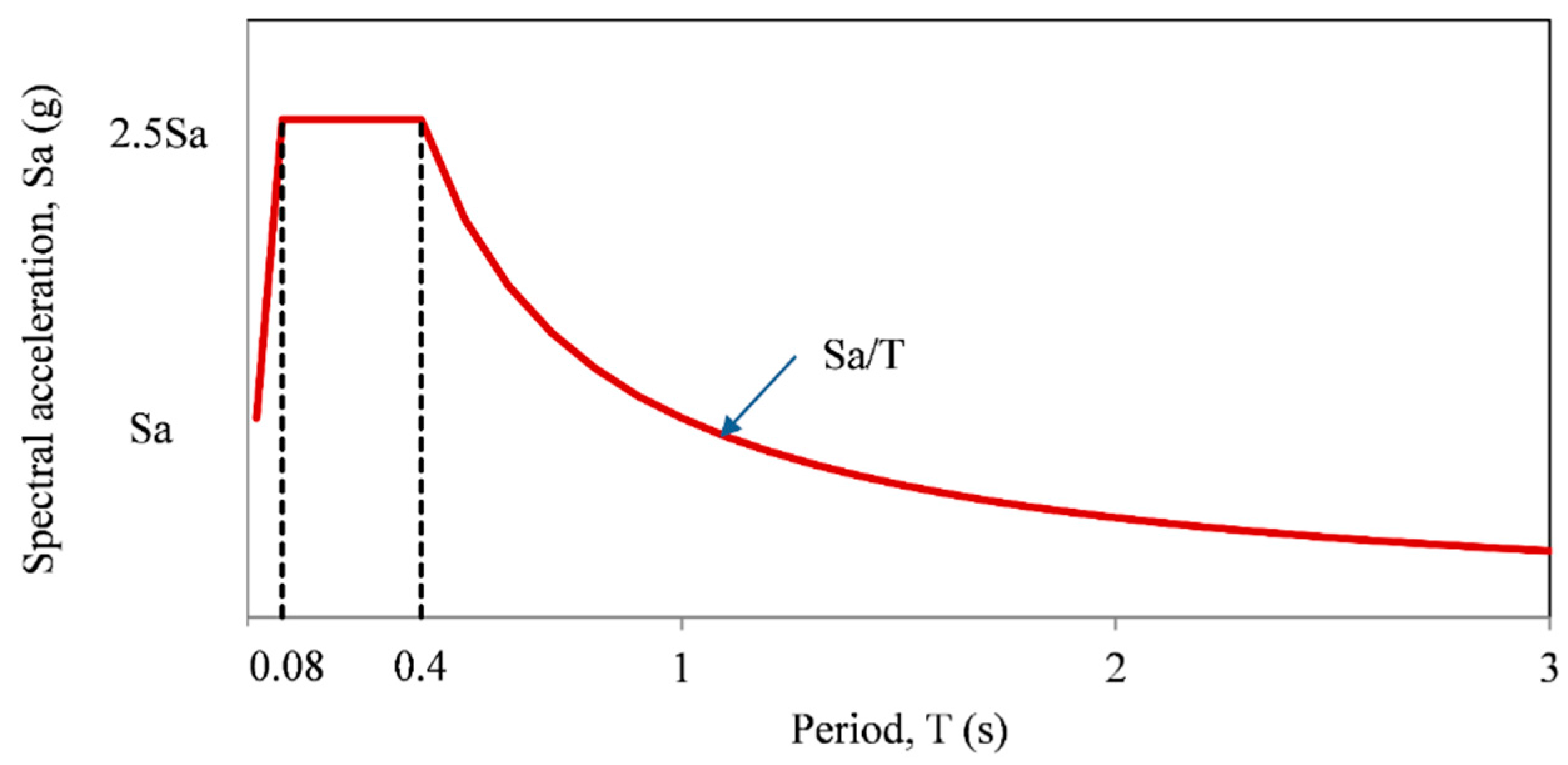
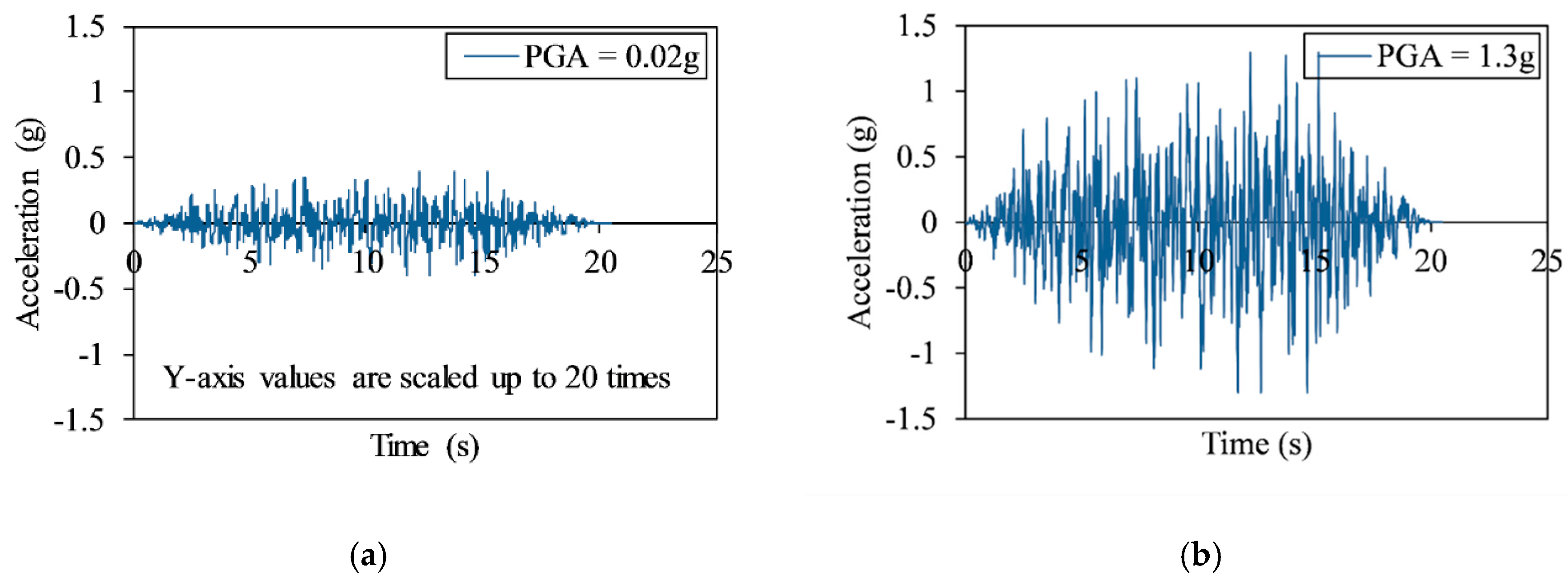
Owing to the lack of sufficient and suitable earthquake records in Korea, a set of artificial ground motions are used in this study to derive the vulnerability curves considering the design spectrum suggested in the Korean Building Code [16], as shown in Figure 3. Twenty-three different seismic PGA levels are considered, and 50 acceleration time histories are artificially generated for each PGA level by using the QuakeGem program [17], which is based on the spectral-representation-based simulation algorithm proposed by Deodatis in 1996 [18,19]. Thus, 1150 ground shaking time histories are produced as inputs to the 1D free-field soil analysis. The PGA level ranges from 0.02 g to 1.3 g. The two minimum and maximum ground motion time histories are illustrated in Figure 4.

2.2. Definition of Damage State of Underground Subway Station

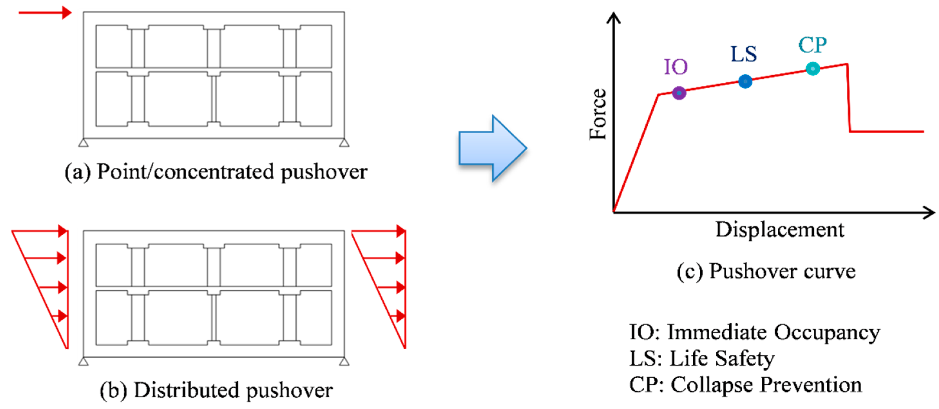
In the pushover analyses, a lateral force is applied incrementally to produce displacements from zero to the ultimate value in order to observe the nonlinear behavior of the structure. The type of lateral force applied on the structure should be selected based on the characteristics of interaction between the soil and structure. For deep tunnels, shear force developed at the exterior surface of the roof is the primary cause of the structural racking deformation. Thus, the racking effects of a deep rectangular tunnel can be simulated by applying a point/concentrated loading at the top of the wall. On the contrary, for a shallow tunnel with a thin overburden soil cover, the racking deformation may be developed along the side walls of the tunnel owing to the normal earth pressures. Therefore, the racking deformation should be imposed by applying an inverse triangular displacement loading along the wall depth [20]. When the structure is buried relatively deep in the soil, both two types of pseudo-static lateral force models (concentrated and inverse triangular force) are expected to be used to produce a unit displacement of the tunnel station, as depicted in Figure 5. The tunnel station is considered as a frame structure, and the plastic hinges are assumed to be developed at the end of the frames. The plastic hinge properties used are those suggested by FEMA 356 [21].

The evaluation of damage is normally based on the deflection response of the structure. The damage states can be divided into three performance levels based on ATC 40 and FEMA 356 [21,22,23], i.e., (a) immediate occupancy (IO), (b) life safety (LS), and (c) collapse prevention (CP), which indicate the correlation between the material nonlinearity and deterministic projections for the structural damage sustained. They can be classified as minor, moderate, and extensive damage states, respectively.

To demonstrate the behavior of a structure, a two-story reinforced concrete tunnel station is modeled by using SAP2000 [24] with the dimensions and details of reinforcement bars depicted in Figure 6. In this program, a post-yield behavior is assigned by concentrated plastic hinges to frames. The inelastic behavior is obtained through integration of the plastic strain and plastic curvature which suggested in FEMA 356. One of the main factors that control the uncertainty of the response of a reinforced concrete structure is the variability of the material strength. The mean and coefficient of variation are used to describe the statistical variation of the material properties. Thus, uncertainties in the design parameters are considered as random variables, and their statistical properties are given in

Table 2. Statistical properties of the random variables.

Random variables	Unit	Distribution	Mean	COV
Elastic modulus of concrete	GPa	Normal	31.23	0.120
Poisson’s ratio of concrete	-	Normal	0.17	0.050
Compression strength of concrete	MPa	Normal	29.42	0.175
Concrete cover	mm	Normal	78.00	0.145
Yield strength of steel	MPa	Log-normal	400.00	0.093
Elastic modulus of steel	GPa	Log-normal	199.95	0.033

[25,26]. In this study, the Latin hypercube approach is applied to simulate the uncertainty and randomness of the random variables. The reason of using this method is that Latin hypercube sampling stratifies the input probability distributions, in which it divides the cumulative curve into equal intervals on the cumulative probability scale, then takes a random value from each interval of the input distribution [27]. Therefore, with a small amount of sample, it shows a good representative of the real variability comparing to the traditional technique such like Monte Carlo Sampling, without sacrificing much accuracy.

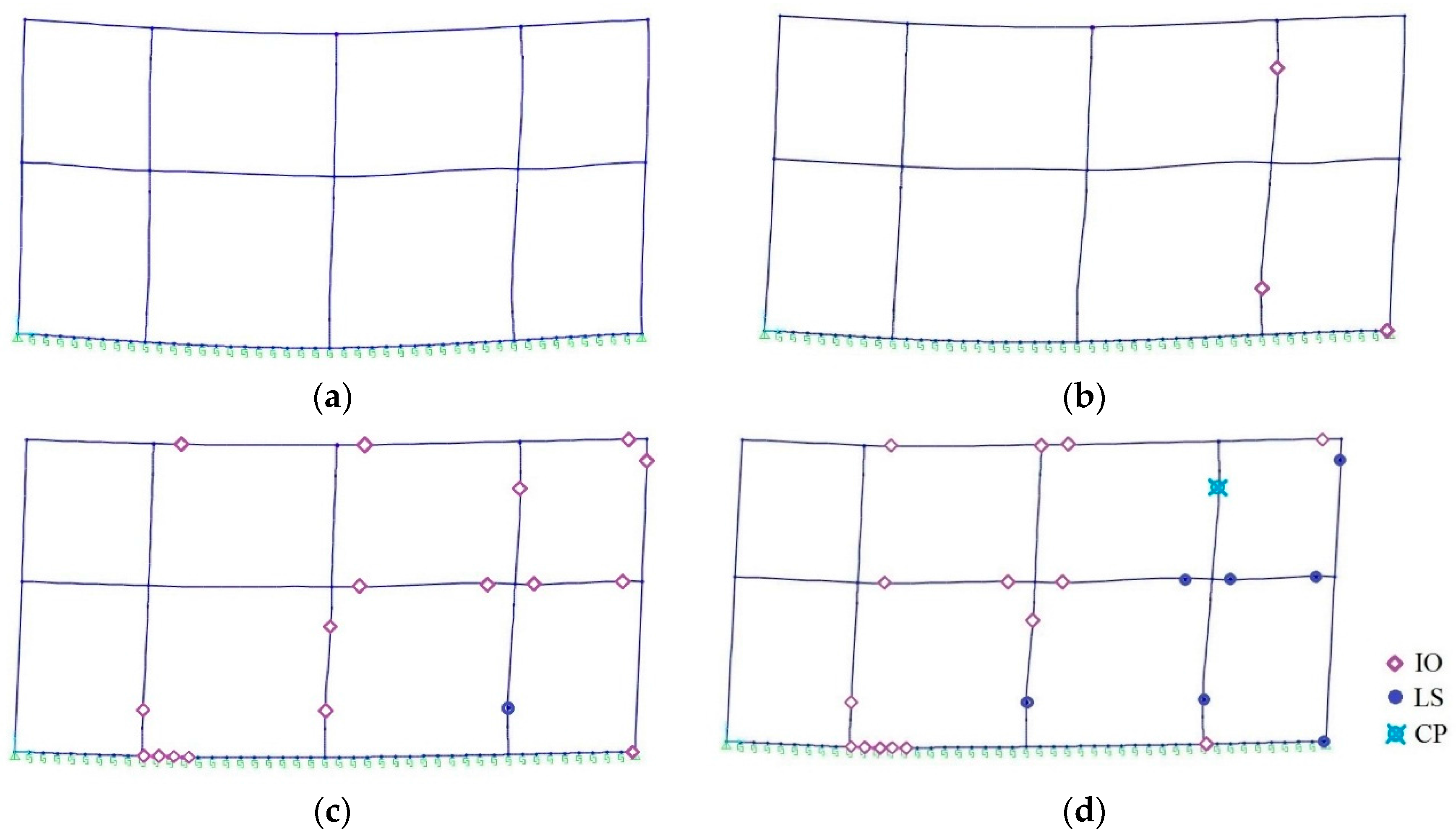
Fifty different pushover analyses per model are conducted. Figure 7 illustrates the deformation of the tunnel and the distribution of plastic hinges in various phases obtained from the pushover analysis. The first hinges of the IO level appear at the joints of the side column and bottom floor as shown in Figure 7b. Under a continuously increasing load, the plastic hinges at the IO level occurred more at several other positions. In addition, a plastic hinge at the toe of the side column first reaches the LS level, as shown in Figure 7c, which causes a potential collapse at the toe of that column. With a gradual increase of load, the most dangerous hinge moves to the top of the same column, reaching the CP level as illustrated in Figure 7d. It indicates that the collapse would first occur at the top of the side column.

Based on the IO, LS, and CP performance level defined in FEMA 356 and ATC 40, the DI is defined as the ratio of the lateral displacement (between the top and bottom of the tunnel) and height of the tunnel in this study. By taking the average of drift capacity values at each performance level, the DI can be derived. The four different damage states are introduced in

Table 3. Definition of damage index (DI).

Damage State	Types of Pseudo-Static Lateral Force
	Concentrated Load	Invert Distributed Load
No damage	DI ≤ 0.11%	DI ≤ 0.13%
Minor	0.11% < DI ≤ 0.36%	0.13% < DI ≤ 0.36%
Moderate	0.36% < DI ≤ 0.88%	0.36% < DI ≤ 0.90%
Extensive	DI > 0.88%	DI > 0.90%

. Under an identical earthquake intensity, the DI from the concentrated load, assuming that the primary cause is due to the shear force developed at the exterior surface of the tunnel roof, reaches the same damage state more easily than the DI from the distributed load, considering that the cause is due to the normal earth pressures developed along the side walls.

3. Fragility Curve Development

The probability of failure or collapse is a conditional probability that the maximum drift between the top and bottom of the tunnel exceeds the drift threshold under the earthquake intensity. After calculating the probability of exceedance of the limit states for each PGA, the vulnerability curve can be constructed by plotting the calculated data versus PGA. There are parametric (e.g., log-normal function) and non-parametric method (e.g., binned Monte Carlo simulation and Kernel density estimation [28]) to establish fragility curve. In this study, the log-normal cumulative distribution function is used to define the fragility function [29,30,31,32,33].

$$\mathrm{P}\left(\mathrm{PGA}=\mathrm{x}\right)=\mathsf{\Phi }\left(\frac{\ln \left(\mathrm{x}/\mathsf{\theta }\right)}{\mathsf{\beta }}\right),$$

(6)

where P(PGA = x) represents the probability that a ground motion with PGA = x causes the structure to collapse; $\mathsf{\Phi }()$ is the standard normal cumulative distribution function; θ and β are the median and standard deviation of ln(PGA), respectively.

At each PGA = x_j, the structural analyses produce some number of collapses out of the total number of ground motions. The probability of observing collapses or no collapses is given by the binomial distribution. Hence, the MLE function is

$$\mathrm{Likelihood}={\displaystyle \prod _{\mathrm{j}=1}^{\mathrm{m}}\left(\begin{array}{c}{\mathrm{n}}_{\mathrm{j}}\\ {\mathrm{z}}_{\mathrm{j}}\end{array}\right)}{\mathrm{p}}_{\mathrm{j}}^{{\mathrm{z}}_{\mathrm{j}}}{\left({1-\mathrm{p}}_{\mathrm{j}}^{{\mathrm{z}}_{\mathrm{j}}}\right)}^{{\mathrm{n}}_{\mathrm{j}}{-\mathrm{z}}_{\mathrm{j}}},$$

(7)

where p_j represents the probability that a ground motion with PGA = x_j causes the collapse, z_j is the number of collapses out of n_j ground motions, and m represents the number of PGA level. In order to perform this maximization, Equation (6) is substituted to Equation (7), so the fragility parameters are explicit in the likelihood function:

$$\mathrm{Likelihood}={\displaystyle \prod _{\mathrm{j}=1}^{\mathrm{m}}\left(\begin{array}{c}{\mathrm{n}}_{\mathrm{j}}\\ {\mathrm{z}}_{\mathrm{j}}\end{array}\right)}\mathsf{\Phi }{\left(\frac{\ln \left({\mathrm{x}}_{\mathrm{j}}/\mathsf{\theta }\right)}{\mathsf{\beta }}\right)}^{{\mathrm{z}}_{\mathrm{j}}}{\left(1-\mathsf{\Phi }\left(\frac{\ln \left({\mathrm{x}}_{\mathrm{j}}/\mathsf{\theta }\right)}{\mathsf{\beta }}\right)\right)}^{{\mathrm{n}}_{\mathrm{j}}{-\mathrm{z}}_{\mathrm{j}}},$$

(8)

The parameters that maximize this likelihood function also maximize the log of the likelihood. The “$\wedge$” notation denotes an estimate of a parameter:

$$\left\{\stackrel{\wedge }{\mathsf{\theta }},\stackrel{\wedge }{\mathsf{\beta }}\right\}=\arg \max {\displaystyle \sum _{\mathrm{j}=1}^{\mathrm{m}}\left\{\ln \left(\begin{array}{c}{\mathrm{n}}_{\mathrm{j}}\\ {\mathrm{z}}_{\mathrm{j}}\end{array}\right){+\mathrm{z}}_{\mathrm{j}}\ln \mathsf{\Phi }\left(\frac{\ln \left({\mathrm{x}}_{\mathrm{j}}/\mathsf{\theta }\right)}{\mathsf{\beta }}\right)+\left({\mathrm{n}}_{\mathrm{j}}{-\mathrm{z}}_{\mathrm{j}}\right)\ln \left(1-\mathsf{\Phi }\left(\frac{\ln \left({\mathrm{x}}_{\mathrm{j}}/\mathsf{\theta }\right)}{\mathsf{\beta }}\right)\right)\right\}},$$

(9)

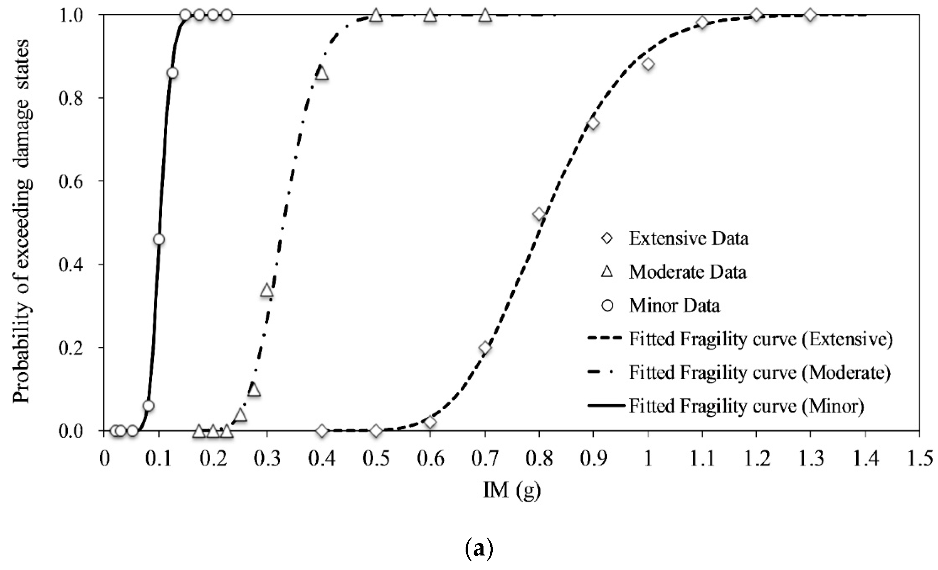
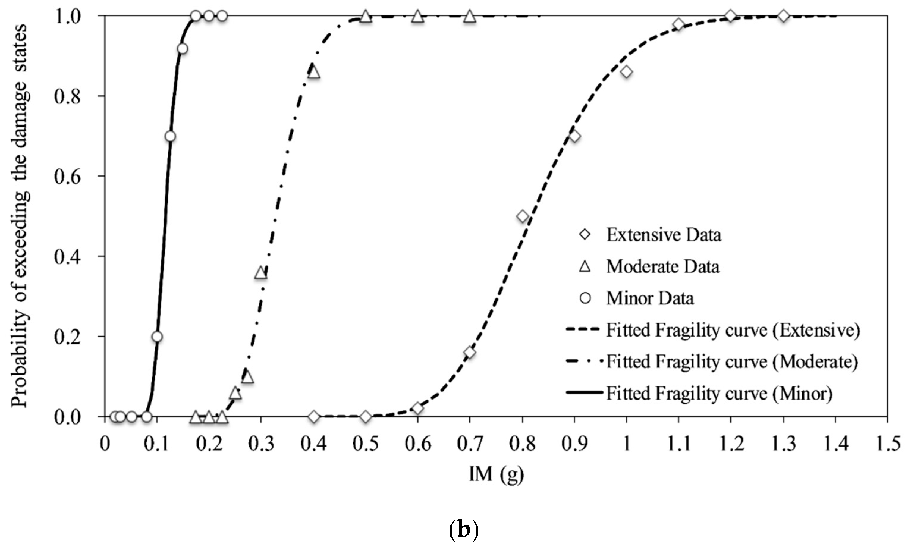
To determine the probability of exceeding the damage states, the resulting displacements of the tunnel obtained by GRAMBS method on twenty-three PGA levels ranging from 0.02 g to 1.3 g as summarized in

Table 4. Number of failures per each PGA level.

PGA (g)	Concentrated			Distributed
	Minor	Moderate	Extensive	Minor	Moderate	Extensive
0.02	0	-	-	0	-	-
0.03	0	-	-	0	-	-
0.05	0	-	-	0	-	-
0.08	3	-	-	0	-	-
0.10	23	-	-	9	-	-
0.13	43	-	-	33	-	-
0.15	50	-	-	46	-	-
0.18	50	0	-	50	0	-
0.20	50	0	-	50	0	-
0.23	50	0	-	50	0	-
0.25	-	2	-	-	3	-
0.28	-	5	-	-	4	-
0.30	-	17	-	-	18	-
0.40	-	43	0	-	41	0
0.50	-	50	0	-	50	0
0.60	-	50	1	-	50	1
0.70	-	50	10	-	50	7
0.80	-	-	26	-	-	25
0.90	-	-	37	-	-	33
1.00	-	-	44	-	-	43
1.10	-	-	49	-	-	49
1.20	-	-	50	-	-	50
1.30	-	-	50	-	-	50
θ	0.103	0.330	0.806	0.116	0.328	0.818
β	0.164	0.157	0.158	0.161	0.161	0.157

Note: θ, β: median and standard deviation of ln(PGA).

, were then compared with the defined damage states as presented in Table 3 for both types of pushover analyses, in order to find the number of failures per each PGA level. Figure 8 shows separately the three fragility curves built from the data of three damage states obtained after the tunnel sustained artificial ground motions, which are indicated by the white circle (for minor), triangular (for moderate), and diamond (for extensive) shapes. A group of ten earthquake PGAs were applied to calculate the three damage states including the minor (PGA from 0.02 g to 0.23 g), moderate (PGA from 0.18 g to 0.7 g), and extensive (PGA from 0.4 g to 1.3 g) states, in which each PGA level contains 50 different artificial earthquakes. As a result, for the concentrated load condition, the median values of PGA (50% probability of exceedance) were 0.103 g, 0.330 g, and 0.806 g for minor, moderate, and extensive damage states respectively, while they were 0.116 g, 0.328 g, and 0.818 g for the distributed load condition, respectively.

In addition, considering the influence of the degree of earthquake intensity increment, there was a significant difference between both pushover models in the minor state. For example, at a PGA of 0.1 g, only 9 minor damage cases happened after sustaining 50 earth shakes under the distributed load case, whereas 23 minor damage cases were expected by the hypothesis of the shear force acting on the tunnel roof. On the other hand, the number of collapse increased significantly with a slight increase in the seismic PGA, especially in the minor and moderate damage states.

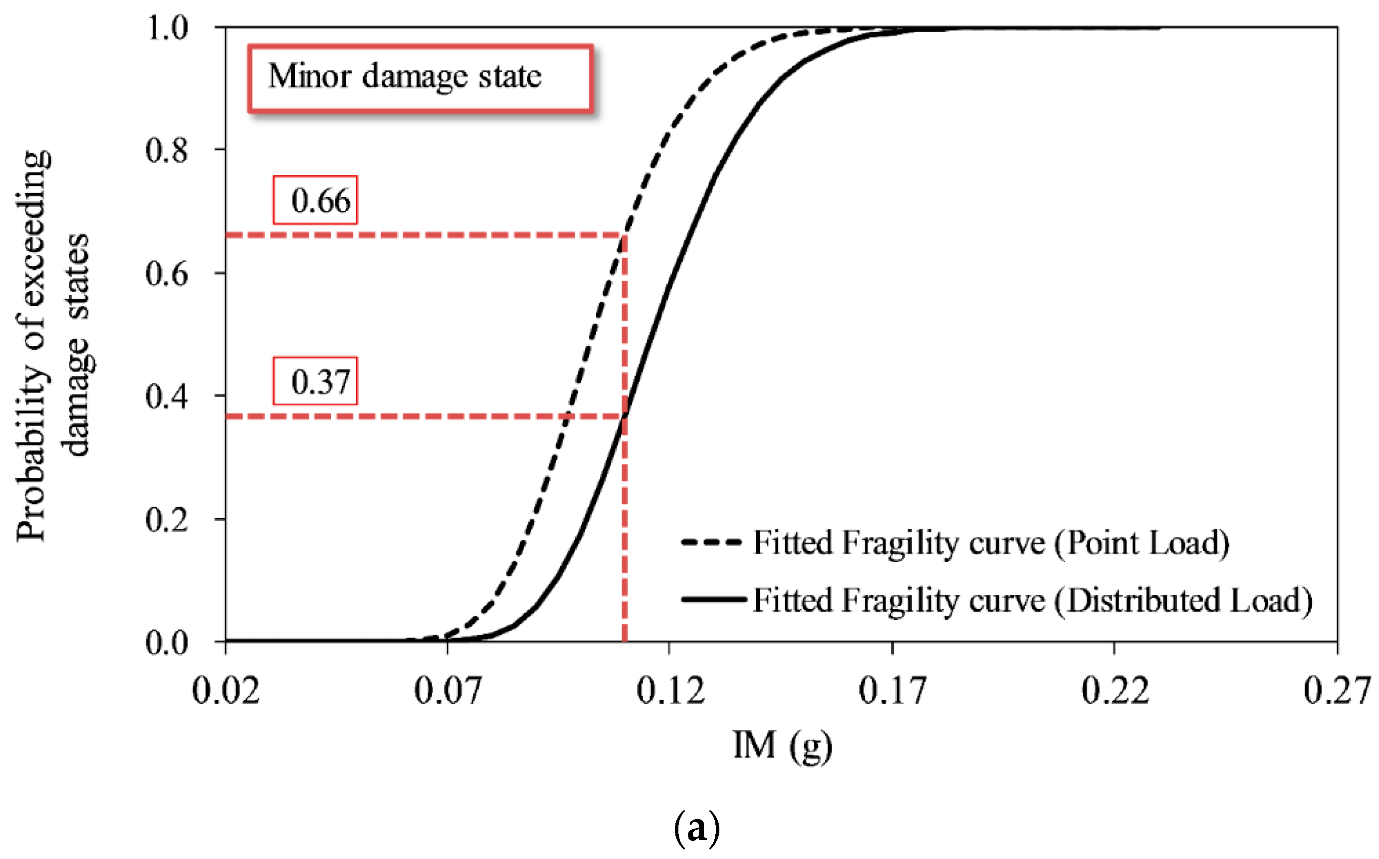
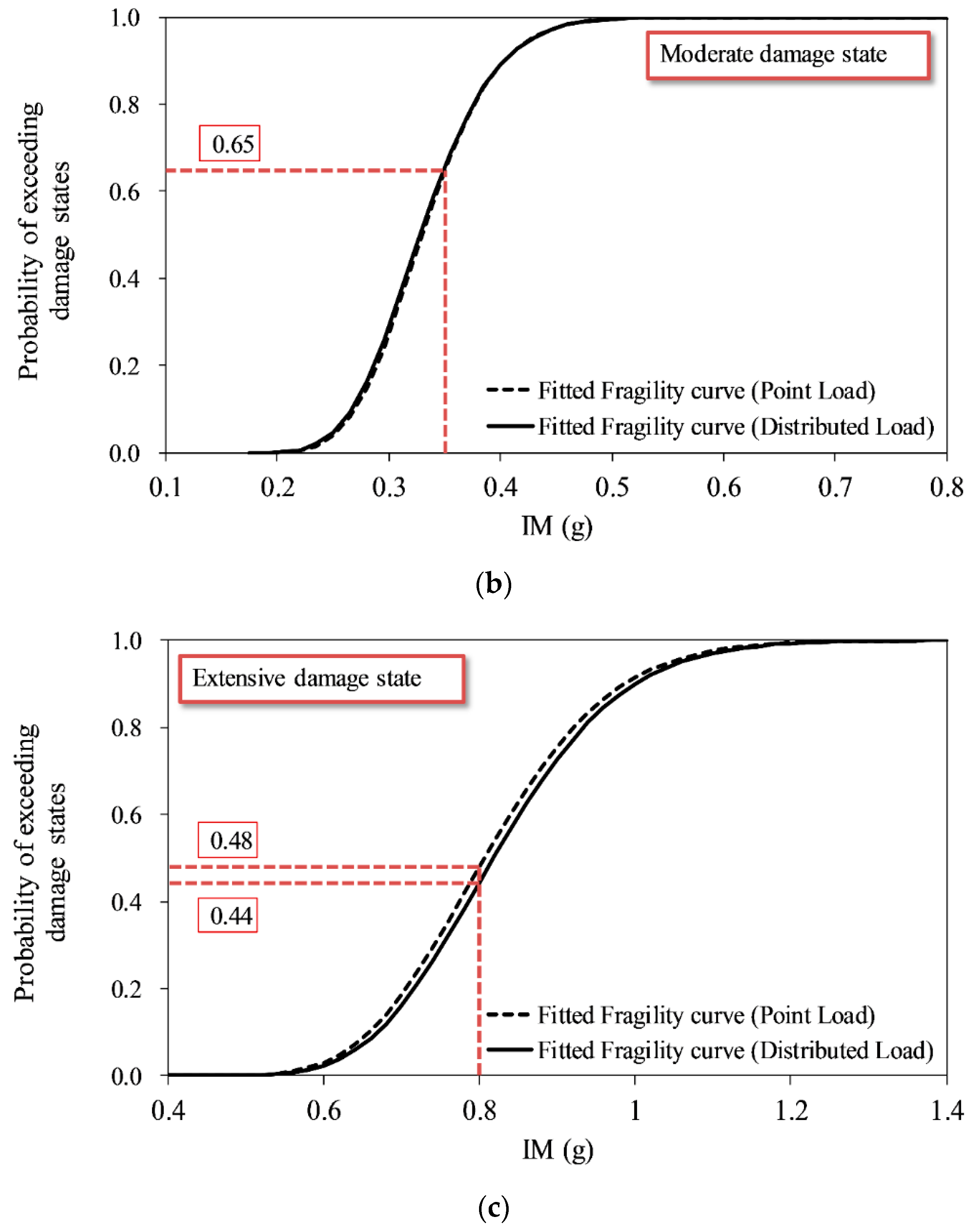
To compare two hypotheses of concentrated load and invert distributed load, the data from Table 4 and the fitted fragility curves from Figure 8 are broken down into three Figure 9a–c. It is clearly seen that the shapes of fragility curves of both hypotheses are similar. However, at the same PGA level, the probability of exceeding the damage state is larger with the point load comparing to the distributed load, except for moderate damage state, it showed nearly same results. For example, in minor damage state, at the same PGA of 0.11 g, the exceedance probability for the point load hypothesis is double the distributed load, which are 66% and 37%, respectively. For extensive state, at the PGA of 0.8 g, they were 48% for point load and 44% for distributed load. The results are similar with a value of 65% for moderate state at a PGA of 0.35 g as shown in Figure 9.

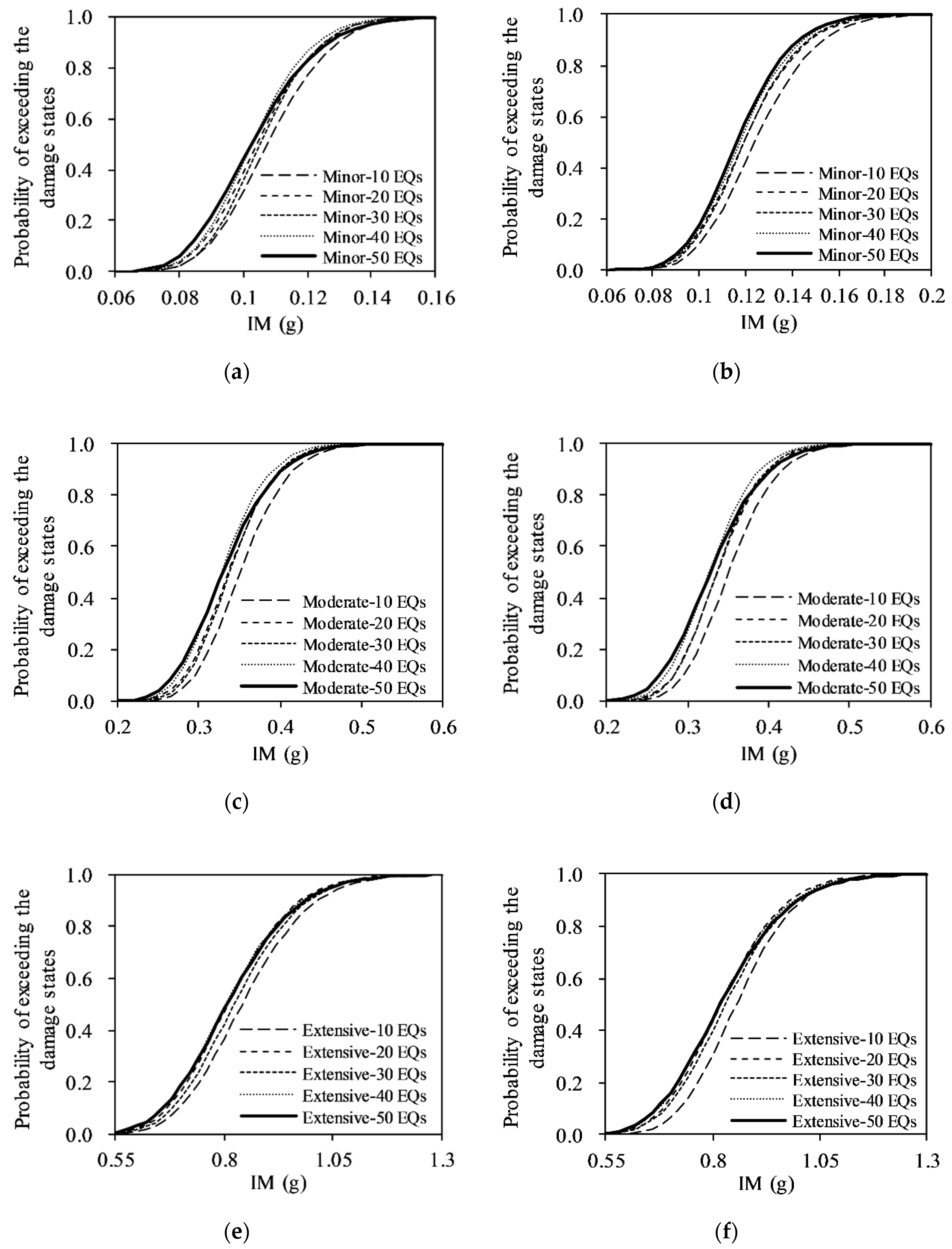
To determine the required number of earthquakes to be applied in practical structural analysis, two statistical parameters, which are required to define a fragility curve, are obtained using the proposed method and three fragility curves, ranging from 10 to 50 earthquakes per PGA level, are derived gradually. The median value at each damage state is acquired with its corresponding log-normal standard deviation value summarized in

Table 5. Fragility curve parameters for 10, 20, 30, 40, and 50 earthquakes per PGA.

Load Type	Concentrated Load						Invert Distributed Load
Earthquakes per PGA		10	20	30	40	50	10	20	30	40	50
Minor	θ	0.107	0.104	0.105	0.103	0.103	0.124	0.119	0.119	0.117	0.116
	β	0.148	0.146	0.137	0.142	0.164	0.167	0.168	0.162	0.162	0.161
Moderate	θ	0.351	0.337	0.338	0.328	0.330	0.351	0.337	0.336	0.327	0.328
	β	0.135	0.137	0.131	0.139	0.157	0.135	0.137	0.133	0.139	0.161
Extensive	θ	0.841	0.809	0.823	0.804	0.806	0.854	0.819	0.830	0.816	0.818
	β	0.148	0.147	0.148	0.155	0.158	0.130	0.142	0.145	0.151	0.157

and plotted in Figure 10.

The fragility curves for the three damage states with a range of 10 to 50 earthquakes per PGA level as illustrated in Figure 10, show similar trends but the lower the number of earthquakes per PGA, the steeper the curves can be observed. Moreover, the cases of 10 earthquakes per PGA show slightly larger values of medians than those for other cases, whereas the cases of equal to or larger than 20 earthquakes per PGA provide more identical values in Figure 10. Therefore, it can be concluded that the analysis with approximately 20 ground motions in each PGA level is a reasonable value for performing the structural analysis to derive the fragility curves of tunnels. In addition, the interval of PGA level is also important to have a good estimation of fragility curve. However, this topic is beyond the scope of this paper.

4. Conclusions

This study examines the fragility curves of a shallow two-story reinforced concrete underground box structure subjected to seismic loading. A total of 1150 artificial ground motions in 23 PGAs ranging from 0.02 g to 1.3 g (with 50 ground motions per PGA level) were applied to a two-dimensional plane strain FEM model.

The effect of the near-field ground domain adjacent to the tunnel structures was investigated to estimate the relative displacement between the top and bottom of the tunnel following the GRAMBS method. An efficient and practical guide based on GRAMBS method, nonlinear static analysis (or pushover) with Latin hypercube sampling, and maximum likelihood method was proposed to construct fragility curves of a RC box structure in a highly-weathered soil. In addition, the definition of damage states was provided by conducting comprehensive pushover analyses with considering the uncertainties of material properties and concrete cover, to help in making a good decision for the recovery time and repair cost, without taking much time for dynamic analysis.

In the comparison of the required earthquakes per PGA level for developing fragility curves, the results suggest that the analysis with equal to or larger than 20 ground motions in each PGA is a reasonable value for performing the structural analyses to derive the fragility curves of tunnels.

The shapes of fragility curves of both hypotheses, the shear force developed at the exterior surface of the roof (point load) and the racking deformation developed along the side walls (invert distributed load), are similar. However, at the same PGA level, the probability of exceeding the damage state of the point load is larger than the distributed load in the minor and extensive damage state, except for the moderate damage state, it shows nearly same results.

In this study, the tunnel material properties and concrete cover had been considered as random variables. This approach can be extended further by considering other uncertainties such as the difference in geometric shapes of underground tunnels owing to a possible incorrect construction or the variability of soil properties.

References

- Yoshida, N.; Nakamura, S. Damage to Daikai Subway Station during the 1995 Hyogoken-Nunbu Earthquake and its Investigation. Proceedings of Eleventh World Conference on Earthquake Engineering, Acapulco, Mexico, 23–28 June 1996. [Google Scholar]
- EQE International. The January 17, 1995 Kobe Earthquake; An EQE Summary Report; EQE International: San Francisco, CA, USA, April 1995. [Google Scholar]
- Matsuda, T.; Tanaka, N. Seismic Response Analysis for a Collapsed Underground Subway Structure with Intermediate Columns. In Proceedings of the 11th World Conference on Earthquake Engineering, Acapulco, Mexico, 23–28 June 1996. [Google Scholar]
- Tsai, Y.; Huang, M. Strong Ground Motion Characteristics of the Chi-Chi, Taiwan Earthquake of 21 September 1999. Earthq. Eng. Eng. Seismol. 2000, 2, 1–21. [Google Scholar]
- Donner, S.; Rößler, D.; Krüger, F.; Ghods, A.; Strecker, M. Source mechanisms of the 2004 Baladeh (Iran) earthquake sequence from Iranian broadband and short-period data and seismotectonic implications. In Proceedings of the AG Seismologie: 37. Meeting, Sankelmark, Germany, 27–29 September 2011. [Google Scholar]
- Earthquake Engineering Research Institute (EERI). Learning from Earthquakes: The Mw 7.0 Haiti Earthquake of 12 January 2010; EERI Special Earthquake Report; Earthquake Science Center: Menlo Park, CA, USA, May 2010.
- Pitilakis, K.; Tsinidis, G. Chapter 11—Performance and Seismic Design of Underground Structures. In Earthquake Geotechnical Engineering Design; Springer: Cham, Switzerland, 2014; pp. 279–340. [Google Scholar]
- Katayama, I. Studies on Fundamental Problems in Seismic Design Analyses of Critical Structures and Facilities. Ph.D. Thesis, Kyoto University, Kyoto, Japan, 1990. [Google Scholar]
- Tateishi, A. A Study on Seismic Analysis Methods in The Cross Section of Underground Structures using Static Finite Elements Method. JSCE 2005, 22, 41–53. [Google Scholar] [CrossRef]
- Kaizu, N.; Annaka, T.; Ohki, H. Observation of behavior of underground power transmission shaft during earthquake. Jpn. Soc. Civ. Eng. 1989, 20, 409–412. (In Japanese) [Google Scholar]
- Ohki, H.; Annaka, T.; TKaizu, N. Analysis of behavior of underground power transmission shaft during earthquake. Jpn. Soc. Civ. Eng. 1989, 20, 413–416. (In Japanese) [Google Scholar]
- Kaizu, N.; Harada, M.; Annaka, T.; Ohki, H. Observation and numerical analyses of shaft for underground transmission lines. PVP (Am. Soc. Mech. Eng.) 1989, 162, 183–190. [Google Scholar]
- Tohma, J. Model experiment of sea water intake duct of nuclear power plant. Denryoku Doboku 1985, 197, 36–44. (In Japanese) [Google Scholar]
- Idriss, I.M.; Sun, J.I. A Computer Program for Conducting Equivalent Linear Seismic Response Analyses of Horizontally Layered Soil Deposits; University of California: Davis, CA, USA, 1992. [Google Scholar]
- MIDAS CIVIL. Technical Lecture; MIDAS Information Technology Co., Ltd.: Gyeonggi, Korea, 2011. (In Korean) [Google Scholar]
- Architectural Institute of Korea. Korean Building Code; Architectural Institute of Korea: Seoul, Korea, 2013. [Google Scholar]
- Kim, J.M. QuakeGem-Computer Program for Generating Multiple Earthquake Motions; Chonnam National University: Gwangju, Korea, 2007. [Google Scholar]
- Deodatis, G. Non-stationary Stochastic Vector Processes: Seismic Ground Motion Applications. Probab. Eng. Mech. 1996, 11, 149–168. [Google Scholar] [CrossRef]
- Deodatis, G. Simulation of Ergodic Multivariate Stochastic Processes. J. Eng. Mech. 1996, 122, 778–787. [Google Scholar] [CrossRef]
- Wang, J.N. Seismic Design of Tunnel-A simple State-of-the-Art Design Approach; Parsons Brinckerhoff Quade & Douglas Inc.: New York, NY, USA, 1993. [Google Scholar]
- Federal Emergency Management Agency (FEMA) 356. Prestandard and Commentary for the Seismic Rehabilitation of Buildings; FEMA: Washington, DC, USA, 2000.
- Applied Technology Council ATC40. Seismic Evaluation and Retrofit of Concrete Buildings; Seismic Safety Commission: Redwood, CA, USA, 1996.
- Freeman, S.A. Review of the development of the capacity spectrum method. ISET J. Earthq. Technol. 2004, 41, 438. [Google Scholar]
- SAP2000. Linear and Nonlinear Static and Dynamic Analysis and Design of 3D Structures: Basic Analysis Reference Manual; CSI: Berkeley, CA, USA, 2006. [Google Scholar]
- Lee, T.H.; Mosalam, K.M. Probabilistic Seismic Evaluation of Reinforced Concrete Structural Components and Systems; PEER Center: Berkeley, CA, USA, 2006. [Google Scholar]
- Matos, J.C.; Batista, J.; Cruz, P.; Valente, I. Chapter 429—Uncertainty Evaluation of Reinforced Concrete Structures Behavior. In Bridge Maintenance, Safety, Management and Life-Cycle Optimization; CRC Press: Boca Raton, FL, USA, 2010; p. 609. [Google Scholar]
- Iman, R.L.; Conover, W. Small sample sensitivity analysis techniques for computer models.with an application to risk assessment. Commun. Stat. Theory Methods 1980, 9, 1749–1842. [Google Scholar] [CrossRef]
- Mai, C.; Konakli, K.; Sudret, B. Seismic Fragility Curves for Structures Using Non-Parametric Representations. Front. Struct. Civ. Eng. 2017, 11, 169–186. [Google Scholar] [CrossRef]
- Baker, J.W. Efficient analytical fragility function fitting using dynamic structural analysis. Earthq. Spectr. 2015, 31, 579. [Google Scholar] [CrossRef]
- Shinozuka, M.; Feng, M.Q.; Kim, H.; Uzawa, T.; Ueda, T. Statistical Analysis of Fragility Curves; University of Southern California: Los Angeles, CA, USA, 2001. [Google Scholar]
- Argyroudis, S.A.; Pitilakis, K.D. Seismic fragility curves of shallow tunnels in alluvial deposits. Soil Dyn. Earthq. Eng. 2012, 35, 1–12. [Google Scholar] [CrossRef]
- Lee, D.H.; Kim, B.H.; Jeong, S.H.; Jeon, J.S.; Lee, T.H. Seismic fragility analysis of a buried gas pipeline based on nonlinear time-history analysis. Int. J. Steel Struct. 2016, 16, 231–242. [Google Scholar] [CrossRef]
- Ibarra, L.F.; Krawinkler, H. Global Collapse of Frame Structures under Seismic Excitations; College of Engineering, University of California: Berkeley, CA, USA, September 2005. [Google Scholar]
Figure 1.
Analytical process of proposed methodology.
Figure 2.
(a) 1D free-field soil response analysis; (b) Plane strain 2D finite element method (FEM) model.
Figure 3.
Typical spectral response acceleration.
Figure 4.
Artificial ground motion time histories with peak ground acceleration (PGA) of (a) 0.02 g and (b) 1.3 g.
Figure 5.
Models of lateral force type and pushover curve: (a) Concentrated load; (b) Inverse triangular load; and (c) Typical pushover curve.
Figure 6.
(a) Typical cross section of the tunnel (in meter); (b) Details of reinforcement bars (in mm).
Figure 7.
An example of deformation and hinges in various phases under inverse triangular loading (a) gravity load; (b) Hinges at immediate occupancy (IO) level; (c) Hinges at life safety (LS) level; and (d) Hinges at collapse prevention (CP) level.
Figure 8.
Fragility curves for damage states: (a) for concentrated load; (b) for Invert distributed load.
Figure 9.
Fitted fragility curves of 50 earthquakes per each PGA level: (a) Minor; (b) Moderate; and (c) Extensive damage state.
Figure 10.
Fragility curves for damage states ranging from 10 to 50 earthquakes per PGA level: (a) Concentrated load (Minor); (b) Distributed load (Minor); (c) Concentrated load (Moderate); (d) Distributed load (Moderate); (e) Concentrated load (Extensive) and (f) Distributed load (Extensive).