Motion Planning for Bipedal Robot to Perform Jump Maneuver

Abstract

The remarkable ability of humans to perform jump maneuvers greatly contributes to the improvements of the obstacle negotiation ability of humans. The paper proposes a jumping control scheme for a bipedal robot to perform a high jump. The half-body of the robot is modeled as three planar links and the motion during the launching phase is taken into account. A geometrically simple motion was first conducted through which the gear reduction ratio that matches the maximum motor output for high jumping was selected. Then, the following strategies to further exploit the motor output performance was examined: (1) to set the maximum torque of each joint as the baseline that is explicitly modeled as a piecewise linear function dependent on the joint angular velocity; (2) to exert it with a correction of the joint angular accelerations in order to satisfy some balancing criteria during the motion. The criteria include the location of ZMP (zero moment point) and the torque limit. Using the technique described above, the jumping pattern is pre-calculated to maximize the jump height. Finally, the effectiveness of the proposed method is evaluated through simulations. In the simulation, the bipedal robot model achieved a 0.477-m high jump.

1. Introduction

Recently, the number of disasters, such as earthquakes and tsunamis, is increasing, and humanoid robots have commonly been expected to work in place of humans in such dangerous environments, in which the terrain can be uneven and unpredictable. Improvement of their locomotion abilities by addition of walking, crawling, climbing, fall protection, and jumping capabilities [1,2,3,4,5,6,7,8,9,10,11,12,13] is important to allow these robots to navigate across such adverse terrain. Unfortunately, most contemporary humanoid robots only have segmental functions. Some robots are designed simply for walking or crawling [2,4,7], while others are designed for jumping alone [9,10]. The purpose of this paper is to add a jumping pattern to a versatile BHR6 robot, which is actuated using electric motors, and that already has walking, rolling, and fall protection capabilities [11,12,13].

Quick and harmonized coordination of the jumper’s body segments is essential for jumping tasks. Humans take advantage of the elasticity of their tendons to store and use kinetic energy during jumping motions. Jumping using elastic elements has been studied intensively. Raibert and colleagues studied hopping robots [14] that were driven by pneumatic and hydraulic actuators to perform various actions, including somersaults [15]. Other researchers successfully demonstrated jumping motions using robots with artificial muscles [16,17]. Curran [9] and Ugurlu [18] proposed jumping mechanisms that use the potential energy of a spring. These research efforts are focused on development of a jumping mechanism and its control. All of these robots have elastic mechanisms that are used to retrieve kinetic energy during dynamic movement cycles. Use of elastic elements has obvious advantages for storage and use of kinetic energy, but they may also affect the performance of the fundamental functions of the robots, e.g., walking, crawling, climbing, and carrying objects. Because our intention is to add jumping functionality to an already versatile robot BHR6 without any elastic mechanism, the robot is modeled as three rigid planer links.

A jumping robot not only requires a high torque output to accelerate its COM (center of mass) at the beginning of the motion but also must realize a high velocity at the end of the motion. As the joints become increasingly extended, the transfer of the joint angular motion to produce the desired translation of the COM becomes less effective. When the joint is fully extended, the effect of this joint on the COM’s translational motion in a specific direction is equal to zero. When these factors are taken into consideration, an appropriate reduction gear is required for the motor [19].

The prime criterion for the robot’s obstacle negotiation ability is the required height of the jump, which is dependent on the vertical velocity of the robot’s COM at the moment when its feet leave the ground. During the push-off phase, when the mechanical limitations are considered, a high-torque output is required to generate high angular acceleration. Sakka et al. proposed an adaptation of human jumping motion based on the ground force [8]. Using a similar algorithm, Okada et al. designed a nonlinear gear ratio profile to maximize the ground force [19]. Ugurlu et al. used the base resonance frequency to realize high acceleration [18]. By addition of elastic devices, Hondo et al. realized jumping motion in the low-power humanoid robot Nao [20] that would not originally have had sufficient power to jump. All these methods planned jump patterns based on the trajectory of the leg length or the force of the ground. It leads to the lack of consideration of each joint state, e.g., the torque, velocity and acceleration. Consequently, the relevant motors could not work in the ultimate states required to supply higher kinetic energy and thus achieve a higher jump. To produce as much energy as possible, an optimal motion pattern is generated by commanding every joint torque as much as possible to match the profile of the motor torque speed curve.

During the push-off phase of the jump, the robot must keep stable. Okada kept the trunk upright while the shank and thigh have the same length [19]. Urata and his colleagues at the University of Tokyo Jouhou System Kougaku Laboratory, used the same method [21]. Nunez planned COM above the ankle to prevent it from falling [22]. Ugurlu proposed a ZMP-based jumping controller design method [23,24]. The ZMP is defined as the point on the ground about which the sum of all the moments of the active forces equals zero. The ZMP always exists inside the support polygon form by all contact points. The distance from the ZMP to the boundary of the support polygon directly influence the stability of the robot. A larger distance leads to a more stable state. Our strategy is based on fine-tuning of the joint torque on the basis of the maximum torque being limited by the motor characteristics while minimizing the cost function via ZMP constraints.

In this paper, we introduce a motion planning method to allow a bipedal robot to perform a jump maneuver without the use of elastic elements. Using the premise of dynamic balance, we command each joint torque as much as possible to match the motor torque speed curve to ensure that the robot can jump to the greatest possible height. In Section 2, we present the robot model that is used in this paper. The method used to generate the jumping pattern is described in detail in Section 3. In Section 4, using playback of an offline pattern that was generated in the previous section, we present experimental results for a bipedal robot model of jumping about 0.477-m-high. We draw conclusions and address our future plans in Section 5.

2. Robot Model

In this section, we present the physical model to be used in this study, along with the assumptions that are made in our analysis. Throughout the complete jumping pattern, by keeping the robot symmetrical with respect to the sagittal plane [18,22], the movements, torques and forces acting on each leg will be identical. This restriction helps us to study jumping using a simplified model that contains only half of the robot.

2.1. Mechanical Model

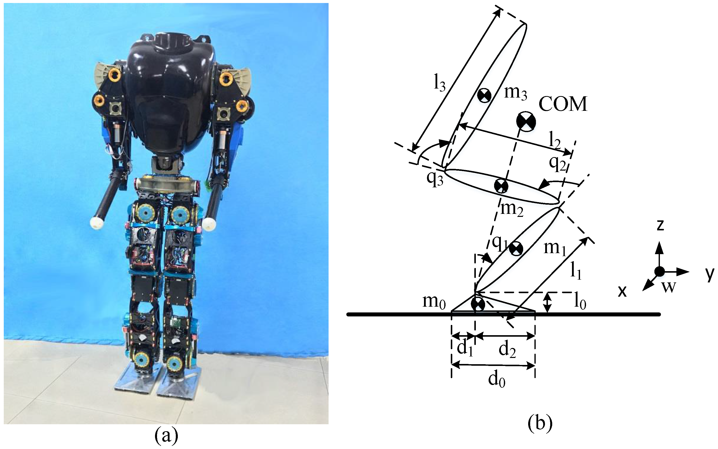
The BHR6 robot and its simplified physical model are shown in Figure 1. Referring to the physical properties of BHR6, we built a model of four links (foot, shank, thigh and trunk) and three articulations (ankle, knee and hip). The foot length is $d_0$, and $d_1,d_2$ represent the distances from the projection of ankle joint on the ground to the heel and tiptoe, respectively. We therefore find that $d_0=d_1+d_2$. The parameter $l_0$ represents the vertical distance from the ankle joint to the ground and $m_0$ is the mass of foot. Additionally, $m_i(i=1,2,3)$ and $l_i(i=1,2,3)$ are the masses and lengths of the shank, the thigh and the trunk, respectively, and the mass center of each link is located at its center. Note also that $m_3$ is only half of the mass of the robot trunk. The model information is listed in detail in

Table 1. Parameters of the simplified model.

${\mathit{m}}_0$	${\mathit{m}}_1$	${\mathit{m}}_2$	${\mathit{m}}_3$	${\mathit{l}}_0$	${\mathit{l}}_1$	${\mathit{l}}_2$	${\mathit{l}}_3$	${\mathit{d}}_0$	${\mathit{d}}_1$	${\mathit{d}}_2$
0.5 (kg)	5.0 (kg)	5.0 (kg)	15 (kg)	0.12 (m)	0.33 (m)	0.33 (m)	0.75 (m)	0.30 (m)	0.10 (m)	0.20 (m)

. The total mass and height of the robot are 51 (kg) and 1.53 (m), respectively.

2.2. Mathematical Model

During the push-off phase, assuming that the friction between the robot foot and the ground is sufficient, the robot will not slide on the ground. Additionally, if the robot foot remain flat on the ground, the model can be represented as a three-part linkage that is fixed to the ground [18,22]. The dynamic equation is given by

$$M(q)\ddot{q}+V(q,\dot{q})+G(q)=F,$$

(1)

where the inertia matrix $M\in R^{3\times 3}$, the coriolis and centripetal coupling vector $V\in R^{3\times 1}$, and the gravity vector $G\in R^{3\times 1}$ are not dependent on the state of the foot. These matrices can be calculated using physical parameters from Table 1 and the instantaneous leg configuration. In this work, we represent all vectors of position, velocity, acceleration, angle, angular velocity and angular acceleration within the world frame ${\sum }_w$. We define the angle, the angular velocity and the angular acceleration of each joint as $q_i$, ${\dot{q}}_i$, and ${\ddot{q}}_i(i=1,2,3)$, respectively. $q={(q_1,q_2,q_3)}^T$ represents the generalized coordinates and $F={({\tau }_1,{\tau }_2,{\tau }_3)}^T$ represents the joint torque.

3. Method

A jumping robot not only requires a high torque output to accelerate its COM at the beginning of the motion but also must realize a high velocity at the end of the motion [19]. From this viewpoint, (1) we selected the appropriate reduction ratio for a specific motor by using a simplified control system; and (2) using the appropriate reduction ratio, a jumping pattern was generated by commanding each motor produces as much kinetic energy as possible within the limitations of the motor properties and dynamic balance throughout the complete push-off phase.

3.1. Selection of an Appropriate Reduction Ratio

Okada et al. designed a nonlinear gear ratio profile with the aim of performing a high jump using direct current motors [19]. However, this profile led to major difficulties in mechanical design, processing and assembly. Our purpose in this work is to determine an appropriate reduction ratio for a specific motor without consideration of the energy transfer efficiency of the gear reducer.

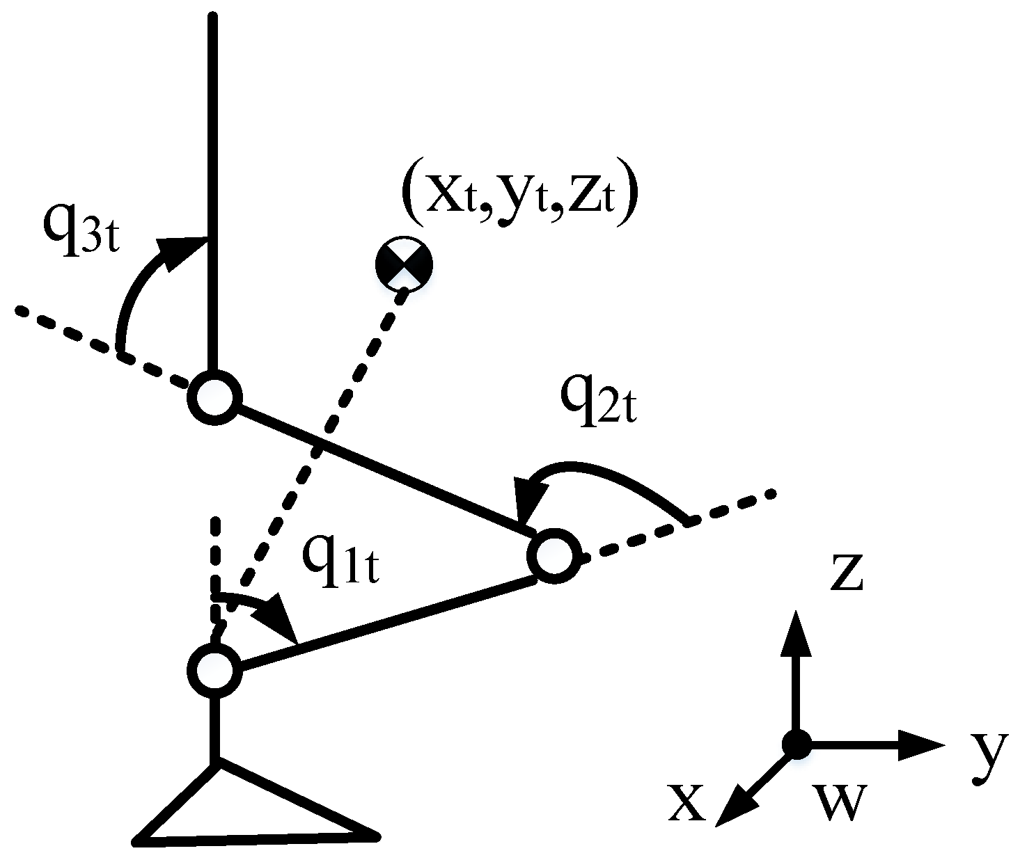
Because of the nonlinearity of the dynamic equation, i.e., Equation (1), it is difficult to determine three appropriate reduction ratios for three motors simultaneously. With reference to the work of Okada and Urata [19,21], we designed a simple jumping pattern in which the trunk remains upright and above the ankle joint during the push-off phase, as shown in Figure 2. In this simple pattern, we can then estimate that of the three joints, and the knee joint will output the maximum torque and speed.

The BHR6 is equipped with the same motor K044100-6Y-4.98Ams (Parker Hannifin Corp, Clifford, OH, USA) on the ankle, knee and hip joint. In Figure 3, according to the instructions from Parker Hannifin, we showed the torque speed curve and properties of motor K044100-6Y-4.98Ams when the voltage supplied to this motor is 120 V. The blue line is the peak output torque of the motor and the red line is the continue output torque of the motor. Because jumping is a fast and dynamic motion, the peak output torque is used in the push-off phase. By the using of the motor driver, the motor can work at an arbitrary point in the right trapezoid formed by the blue line and axis.

From Figure 3, the peak torque speed curve of this motor can be modeled as a segmented function. When the motor speed ${\omega }_{motor}\le {\omega }_{break}({\omega }_{break}=$ 10634 (rpm)), the peak motor torque ${\tau }_{motor}$ is ${\tau }_{peak}=$ 1.17 (Nm). When ${\omega }_{motor}\in [{\omega }_{break},{\omega }_{max}]$ (${\omega }_{max}=18835$ (rpm)), ${\tau }_{motor}$ decreases linearly with increasing ${\omega }_{motor}$. Given these parameters, we can then obtain the relationship between ${\omega }_{motor}$ and ${\tau }_{motor}$, as shown below:

$${\tau }_{motor}=\left\{\begin{array}{cc}{\tau }_{peak}\hfill & {\omega }_{motor}\le {\omega }_{break},\hfill \\ {\tau }_{peak}-\frac{{\tau }_{peak}\ast {\omega }_{motor}}{({\omega }_{max}-{\omega }_{break})}\hfill & {\omega }_{motor}\in [{\omega }_{break},{\omega }_{max}].\hfill \end{array}\right.$$

(2)

We used the harmonic reducer to deliver the motor torque. If the reduction ratio applied to the motor is $i_r$, then the joint speed ${\omega }_{joint}$ will be $\frac{1}{i_r}$ of the ${\omega }_{motor}$. If the transfer efficiency of reducer is assumed as 100%, the output power of motor and joint are identical, ${\omega }_{joint}{\tau }_{joint}={\omega }_{motor}{\tau }_{motor}$. In addition, the peak joint torque ${\tau }_{joint}$ will be $i_r$ times as ${\tau }_{motor}$:

$${\tau }_{joint}=i_r{\tau }_{motor}(\mathrm{Nm}),$$

(3)

$${\omega }_{joint}=\frac{{\omega }_{motor}}{i_r}(\mathrm{rpm})=\frac{2\pi {\omega }_{motor}}{60i_r}(\mathrm{rad}/\mathrm{s}).$$

(4)

It is assumed that the model state at time t is $X_t(q_t,\dot{q_t})$. $q_t=(q_{1t},q_{2t},q_{3t})$ (rad) and $\dot{q_t}=({\dot{q}}_{1t},{\dot{q}}_{2t},{\dot{q}}_{3t})$ (rad/s). Parameter $C_t=(x_t,y_t,z_t)$ (m) represents the coordinate of the COM. The translational velocity of the COM ${\dot{C}}_t$ can then be calculated using the COM Jacobian matrix $J(q_t)$:

$${\dot{C}}_t=J(q_t){\dot{q}}_t.$$

(5)

Using the parameters given in Table 1, where $l_1=l_2$, and the simple jumping pattern, we can obtain the joint constraint equations as shown below:

$$\left\{\begin{array}{ccc}\hfill q_{2t}& =\hfill & \hfill -2q_{1t}=-2q_{3t},\\ \hfill {\dot{q}}_{2t}& =\hfill & \hfill -2{\dot{q}}_{1t}=-2{\dot{q}}_{3t},\\ \hfill {\ddot{q}}_{2t}& =\hfill & \hfill -2{\ddot{q}}_{1t}=-2{\ddot{q}}_{3t}.\end{array}\right.$$

(6)

We can estimate that, of the three joints, the knee joint will output the maximum torque and speed. Using the basic idea of maintaining the knee joint torque’s compliance with the motor torque speed curve, we substitute ${\dot{q}}_{2t}$ into Equations (2)–(4) to calculate the peak knee joint torque ${\tau }_{2t}$ (Nm) at time t:

$${\tau }_{2t}=\left\{\begin{array}{cc}{\tau }_{peak}{i}_r\hfill & {\dot{q}}_{2t}\le \frac{2\pi {\omega }_{break}}{60i_r},\hfill \\ {\tau }_{peak}{i}_r-\frac{60{\tau }_{peak}{i}_r^2{\dot{q}}_{2t}}{2\pi ({\omega }_{max}-{\omega }_{break})}\hfill & {\dot{q}}_{2t}\in [\frac{2\pi {\omega }_{break}}{60i_r},\frac{2\pi {\omega }_{max}}{60i_r}].\hfill \end{array}\right.$$

(7)

With the joint constraint of Equation (6), the second row of Equation (1) then becomes

$$\left(\begin{array}{ccc}{M}_{21}& M_{22}& M_{23}\end{array}\right)\left(\begin{array}{c}-0.5\\ 1\\ -0.5\end{array}\right){\ddot{q}}_{2t}+V_2+G_2={\tau }_{2t},$$

(8)

where $V_2,G_2$ represent the second rows of $V,G$ in state $X_t$, respectively. $M_{ij}(i=2,j=1,2,3)$ is the i-th row and j-th column element of M. Therefore, the maximum angular acceleration ${\ddot{q}}_{2t}$ of the knee joint at time t is

$${\ddot{q}}_{2t}=\frac{{\tau }_{2t}-V_2-G_2}{\left(\begin{array}{ccc}{M}_{21}& M_{22}& M_{23}\end{array}\right)\left(\begin{array}{c}-0.5\\ 1\\ -0.5\end{array}\right).}$$

(9)

Using the joint constraint Equation (6), we can get the $q_t$, ${\dot{q}}_t$ and ${\ddot{q}}_t$ at time t. Thus, the torque of each joint ${\tau }_t=({\tau }_{1t},{\tau }_{2t},{\tau }_{3t})$ then becomes

$${\tau }_t=M(q_t){\ddot{q}}_t+V(q_t,{\dot{q}}_t)+G(q_t).$$

(10)

Obviously, the knee joint torque ${\tau }_{2t}$ is equal to the peak torque limited by motor characteristics. By taking the derivative of Equation (5) with respect to t, we can calculate the translational acceleration of COM ${\ddot{C}}_t$ at time t:

$${\ddot{C}}_t=\dot{J}(q_t){\dot{q}}_t+J(q_t){\ddot{q}}_t.$$

(11)

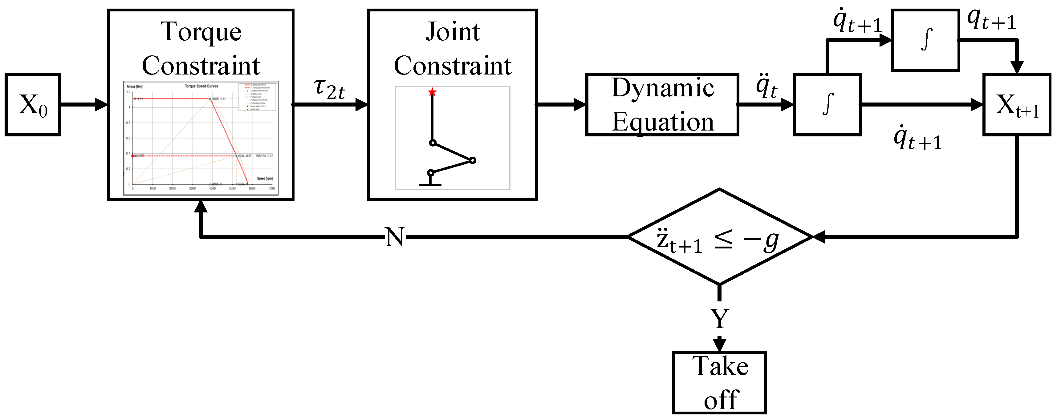
Integration of ${\ddot{q}}_t$ with respect to t allows the next moment state $X_{t+1}(q_{t+1},{\dot{q}}_{t+1})$ to be obtained. Therefore, by providing the initial state $X_0(q_0,{\dot{q}}_0)$, we can then calculate iteratively the $X_t$, ${\ddot{q}}_t$, ${\tau }_t$, $C_t$, ${\dot{C}}_t$, and ${\ddot{C}}_t$ throughout the entire push-off phase, which guarantees that the COM maintains maximum acceleration. The control system is shown in Figure 4.

Since our objective is to jump, we have to detect the take-off time to make the robot foot free when the robot is going to take off. At the beginning of the motion, the ${\ddot{z}}_t$ is positive and the COM is accelerated. When the leg is going to full extension, the ${\ddot{z}}_t$ will decrease rapidly. Since the computation is iterative and has a certain computation period, the take-off time most likely exists within one of the computation periods. The vertical acceleration of COM calculated is ≤$-g$ before the take-off time, and ≤$-g$ after the take-off time. In addition, ${\ddot{z}}_{t+1}\le -g$ is a condition that only happens in mathematical calculations not in the real jump motion. If we get a vertical acceleration of COM, which is ≤$-g$ during the push-off phase, it means that the robot has left the ground. The jump height h is then estimated as

$$h=\frac{{\dot{z}}_{takeoff}^2}{2g},$$

(12)

where ${\dot{z}}_{takeoff}$ is the vertical velocity of the COM at the take-off time and g is the acceleration due to gravity.

To select the appropriate reduction ratio, we define the same initial state $X_0$ = ($-{75}^{\circ }$, ${150}^{\circ }$, $-{75}^{\circ }$, 0, 0, 0) for different values of the reduction ratio $i_r$. The results of the relationship between h and $i_r$ can then be presented graphically. Referring to Figure 5, it shows that when $i_r=97$, the maximum jump height is approximately $h_{max}=0.343$ (m). However, the gear reduction ratio has only certain specific values, e.g., 30, 50, 80, 100, and 120. Finally, therefore, we choose the most appropriate reduction ratio of $i_r=100$.

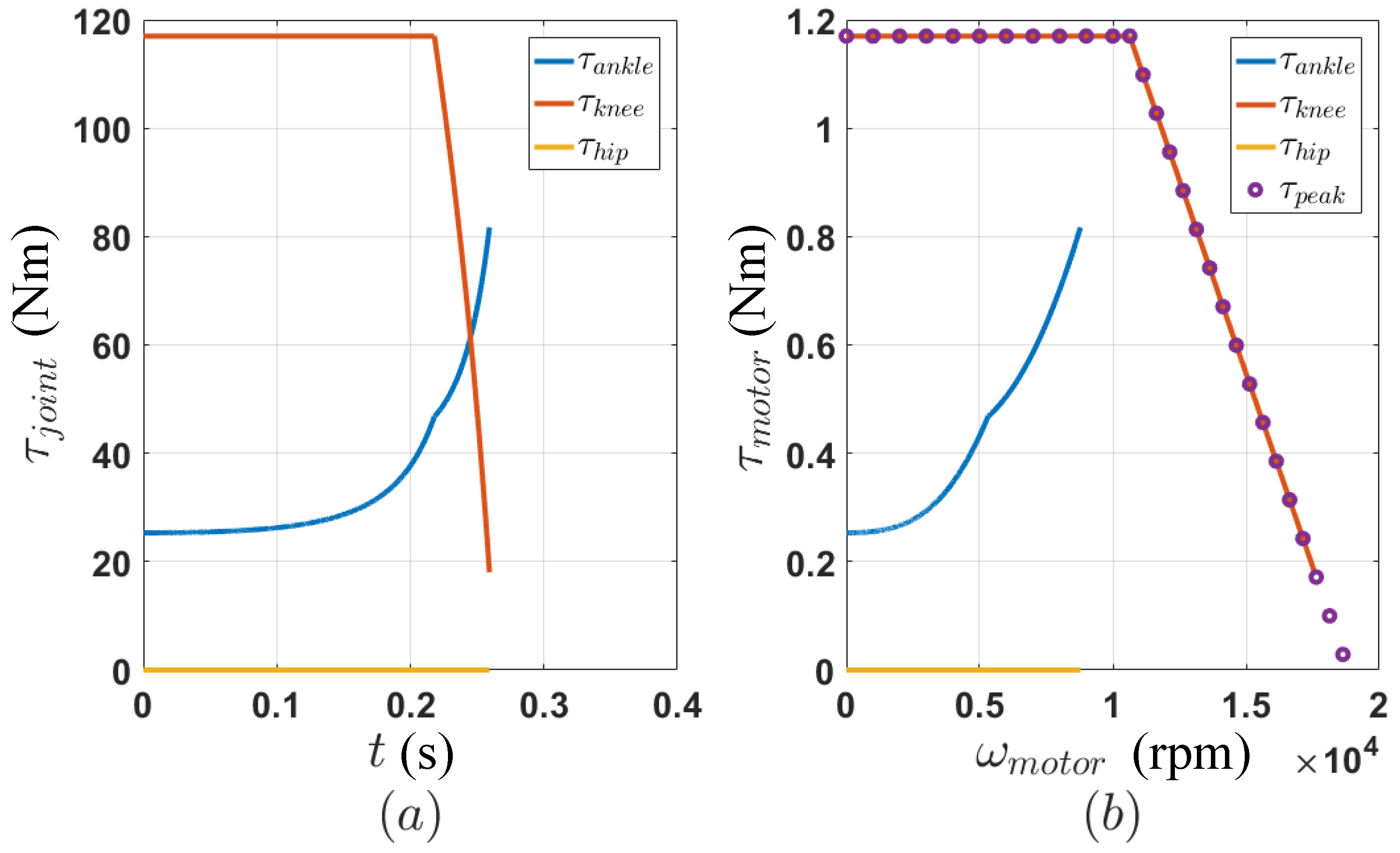
Most of the robots are equipped with the same or similar motor and reduction ratio on these three joints, e.g., NAO [20], HRP3L [21], DARwin [25] and Honda E2-DR [26] . We equip these three joints with the same K044100-6Y-4.98Ams motor and the same reduction ratio of $i_r=100$. Using the control system shown in Figure 4, we obtain the torques of the three joints over the entire push-off phase, as shown in Figure 6. In Figure 6b, the purple circle ${\tau }_{peak}$ is the peak output torque of the motor. The other three lines are composed by the working points of three joints when the robot jumps. All the working points are always in the right trapezoid form by ${\tau }_{peak}$ and axis. Furthermore, as expected, the knee joint torque coincides with the maximum torque permitted by the motor’s characteristics. However, the ankle and hip motors are ineffective as suppliers of kinetic energy. The hip joint doesn’t work and its torque is a constant 0 (Nm), while the ankle joint works at a low efficiency and its torque is much less than the maximal torque allowed. To address this problem, we removed the joint constraint of Equation (6) and take the ZMP constraint into consideration. The details are described in the Section 3.2.

3.2. Motion Planning for Jumping Maneuver

In the original control system in Figure 4, under the joint constraint of Equation (6), we could only ensure that the knee joint torque matched the ultimate torque. To ensure that all three joint torques yield the torque speed curve profile simultaneously as much as possible, we removed the joint constraint and commanded each motor output torque to the torque speed curve. Driven by these torques, the robot will turn over. Thus, we added the ZMP constraint to help the robot to be stable in the push-off phase. If the ZMP constraint is violated, we will fine-tune these torques through optimization. If the ZMP constraint is satisfied, we will directly apply these torques to the joints.

We substitute ${\dot{q}}_{1t},{\dot{q}}_{2t},{\dot{q}}_{3t}$ into Equations (2)–(4) to calculate the peak ankle, knee and hip joint torques ${\tau }_{1t},{\tau }_{2t},{\tau }_{3t}$, respectively, at time t. The maximum angular accelerations of the three joints can then be obtained as follows:

$${\ddot{q}}_t=M{(q_t)}^{-1}({\tau }_t-V(q_t,{\dot{q}}_t)-G(q_t)),$$

(13)

where ${\tau }_t=({\tau }_{1t},{\tau }_{2t},{\tau }_{3t})$ represents the peak torques of the three joints within the limitations of the motor characteristics and $M,C,G$ can be calculated with state $X_t(q_t,{\dot{q}}_t)$. Using Equations (5) and (11), the ZMP of the robot at time t can be given as below [24]:

$$\left(\begin{array}{c}{p}_{xt}\\ p_{yt}\\ p_{zt}\end{array}\right)=\left(\begin{array}{c}{x}_t-\frac{(z_t-p_{zt}){\ddot{x}}_t}{{\ddot{z}}_t+g}\\ y_t-\frac{(z_t-p_{zt}){\ddot{y}}_t}{{\ddot{z}}_t+g}\\ 0\end{array}\right),$$

(14)

where $(x_t,y_t,z_t)$ is the coordinate of the COM that can be calculated with $q_t$. Generally, if the joints move with maximum angular acceleration calculated by Equation (13), the $p_{yt}$ may move out of the supporting polygon formed by the feet and the ZMP constraint will be violate. Assuming that the limitation to $p_{yt}$ is $p_{ylim}\in (-0.05,0.15)$ (m), which is smaller than the distances from the projection of ankle joint on the ground to the heel $d_1$ (0.10 (m)) and to the tiptoe $d_2$ (0.20 (m)) as Figure 7 shows.

At time t, according to the state of the robot $X_t(q_t,{\dot{q}}_t)$ and Equation (5), (11) and (14), the ZMP can be expressed as a function of ${\ddot{q}}_t=({\ddot{q}}_{1t},{\ddot{q}}_{2t},{\ddot{q}}_{3t})$. By taking the total derivative, we can get the $\Delta p_{yt}$ as below:

$$\Delta p_{yt}=\frac{\partial p_{yt}}{\partial {\ddot{q}}_{1t}}\Delta {\ddot{q}}_{1t}+\frac{\partial p_{yt}}{\partial {\ddot{q}}_{2t}}\Delta {\ddot{q}}_{2t}+\frac{\partial p_{yt}}{\partial {\ddot{q}}_{3t}}\Delta {\ddot{q}}_{3t}=\sum _{i=1}^3(\frac{\partial p_{yt}}{\partial {\ddot{q}}_{it}}\Delta {\ddot{q}}_{it}).$$

(15)

If $p_{yt}$ is located beside $p_{ylim}$, then the $\Delta {\ddot{q}}_t$ added to ${\ddot{q}}_t$ should satisfy the following equation:

$$-0.05-p_{yt}\le \sum _{i=1}^3(\frac{\partial p_{yt}}{\partial {\ddot{q}}_{it}}\Delta {\ddot{q}}_{it})\le 0.15-p_{yt}.$$

(16)

The same method can also be applied to the joint torque constraint. Due to the dynamic equation and $X_t(q_t,{\dot{q}}_t)$, the joint torque ${\tau }_t$ can be expressed as a function of ${\ddot{q}}_t=({\ddot{q}}_{1t},{\ddot{q}}_{2t},{\ddot{q}}_{3t})$. By taking the total derivative, we can get the $\Delta {\tau }_{it}(i=1,2,3)$ as below:

$$\Delta {\tau }_{it}=\frac{\partial {\tau }_{it}}{\partial {\ddot{q}}_{1t}}\Delta {\ddot{q}}_{1t}+\frac{\partial {\tau }_{it}}{\partial {\ddot{q}}_{2t}}\Delta {\ddot{q}}_{2t}+\frac{\partial {\tau }_{it}}{\partial {\ddot{q}}_{3t}}\Delta {\ddot{q}}_{3t}=\sum _{j=1}^3(\frac{\partial {\tau }_{it}}{\partial {\ddot{q}}_{jt}}\Delta {\ddot{q}}_{jt});(i=1,2,3).$$

(17)

To maintain the torque constraint, the $\Delta {\ddot{q}}_t$ added to ${\ddot{q}}_t$ must satisfy the following equation:

$$|\sum _{j=1}^3(\frac{\partial {\tau }_{it}}{\partial {\ddot{q}}_{jt}}\Delta {\ddot{q}}_{jt})+{\tau }_{it}|\le |{\tau }_{it}|(i=1,2,3),$$

(18)

where ${\tau }_{it}(i=1,2,3)$ is the maximal torque allowed by torque speed curve at speed ${\dot{q}}_{it}(i=1,2,3)$. To get the optimal solution for the set of inequalities composed by Equations (16) and (18), we built a cost function

$$Cost(\Delta {\ddot{q}}_t)=\sum _{i=1}^3\sum _{j=1}^3|\frac{\partial {\tau }_{it}}{\partial {\ddot{q}}_{jt}}\Delta {\ddot{q}}_{jt}{\dot{q}}_{it}|.$$

(19)

Since $|\Delta {\tau }_{it}|$ is the decrease of each joint torque, then $|\Delta {\tau }_{it}{\dot{q}}_{it}|$ will be the decrease of each joint power. The sum decreases of the three joint output power can be expressed as the Equation (19). A smaller value of Equation (19) leads to a more output energy that affects the jump height directly. Using the linear programming, we obtain the optimum $\Delta {\ddot{q}}_t$ required to minimize the cost function of Equation (19) while simultaneously satisfying the the set of inequalities composed by Equation (16) and Equation (18).

Figure 8 shows the control system. In this program process, there is no joint constraint any more. The torque constraint is used to ensure that all three joint torques yield the torque speed curve profile. In addition, the ZMP constraint is used to keep the dynamic balance throughout the entire puss-off phase. From the control system, we can see that the initial state $X_0$ plays an important role in the jump height. We used the traversal method to obtain the jump height for different $X_0(q_{10}\in [-{65}^{\circ },-{30}^{\circ }]$, $q_{20}\in [-{180}^{\circ },{180}^{\circ }],q_{30}\in [-{180}^{\circ },{180}^{\circ }],{\dot{q}}_{10}=0,{\dot{q}}_{20}=0,{\dot{q}}_{30}=0)$. For various initial values of ankle angle $q_{10}\in [-{65}^{\circ },-{30}^{\circ }]$, we got the optimal $q_{20}$, $q_{30}$ and the jump height as shown in Figure 9a–c. With the increasing $q_{10}$, the jump height h increases while $q_{10}<-{57}^{\circ }$ and subsequently decreases. When compared with the original control method, the height h obtained using the proposed method is obviously greater. In particular, at $X_0=(-{57}^{\circ },{158}^{\circ },-{126}^{\circ },0,0,0)$, we obtained a maximum jump height of 0.61 (m). The jumping height is increased by nearly 70%. Additionally, we calculated the jumping direction $\theta$ with

$$\theta =atan2({\dot{z}}_{takeoff},{\dot{y}}_{takeoff}).$$

(20)

Figure 9d shows that the jumping direction $\theta$ and the initial ankle angle $q_{10}$ have an almost linear relationship. Therefore, we can almost control the jumping direction $\theta$ via the initial ankle angle $q_{10}$.

Assuming that $X_0=(-{57}^{\circ },{158}^{\circ },-{126}^{\circ },0,0,0)$, Figure 10 and Figure 11 show the torques of the three joints ${\tau }_i$ and the ZMP $p_y$, respectively, during the entire push-off phase. For most of the motion time, the ankle, knee, and hip joint torques are all equal to the maximal torques allowed by motors, which greatly increases the kinetic energy. At the beginning of the jump motion, we can see the effectiveness of the control system, which reduces the ankle joint torque slightly to satisfy the ZMP constraint. Similar effectiveness can also be observed when the robot is about to take off. During the whole push-off phase, the working points of three joints are always in the right trapezoid form by ${\tau }_{peak}$ and axis.

4. Simulation Results

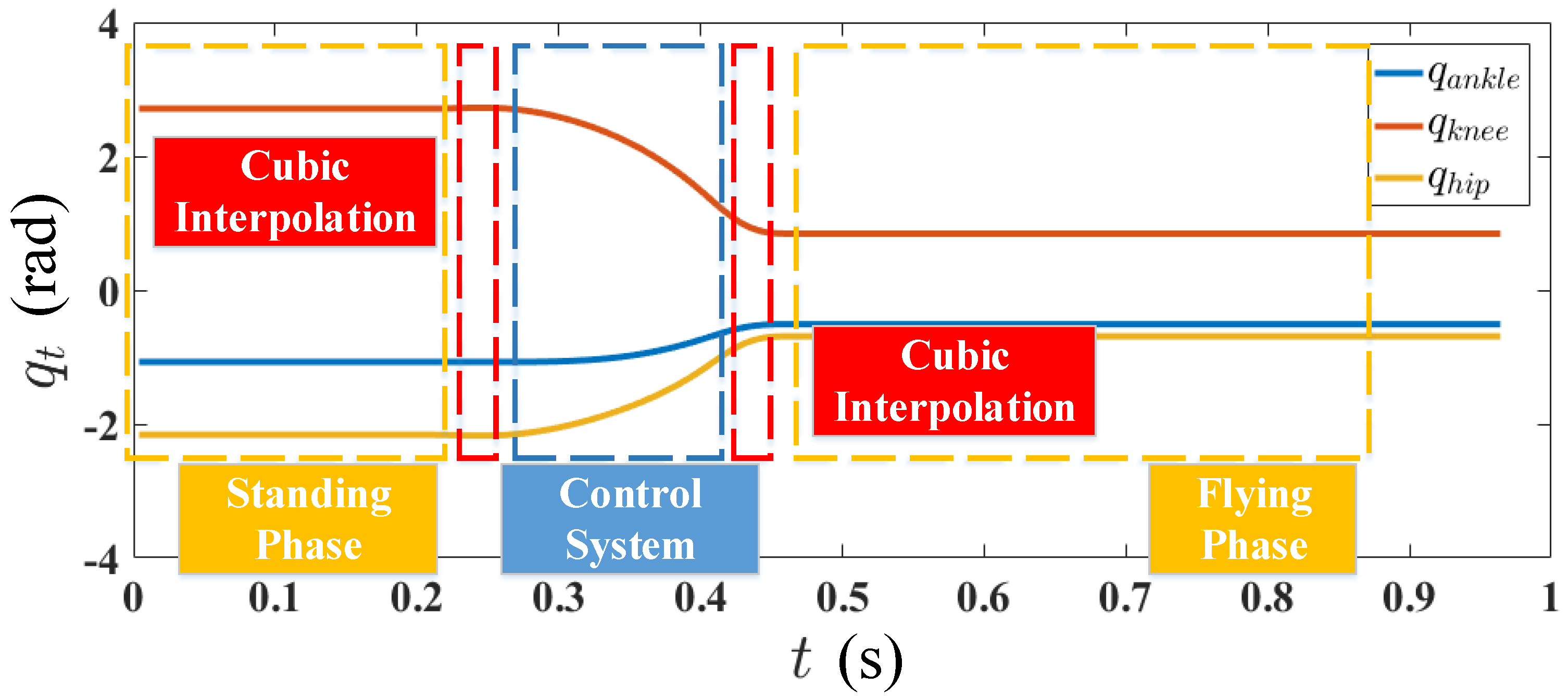
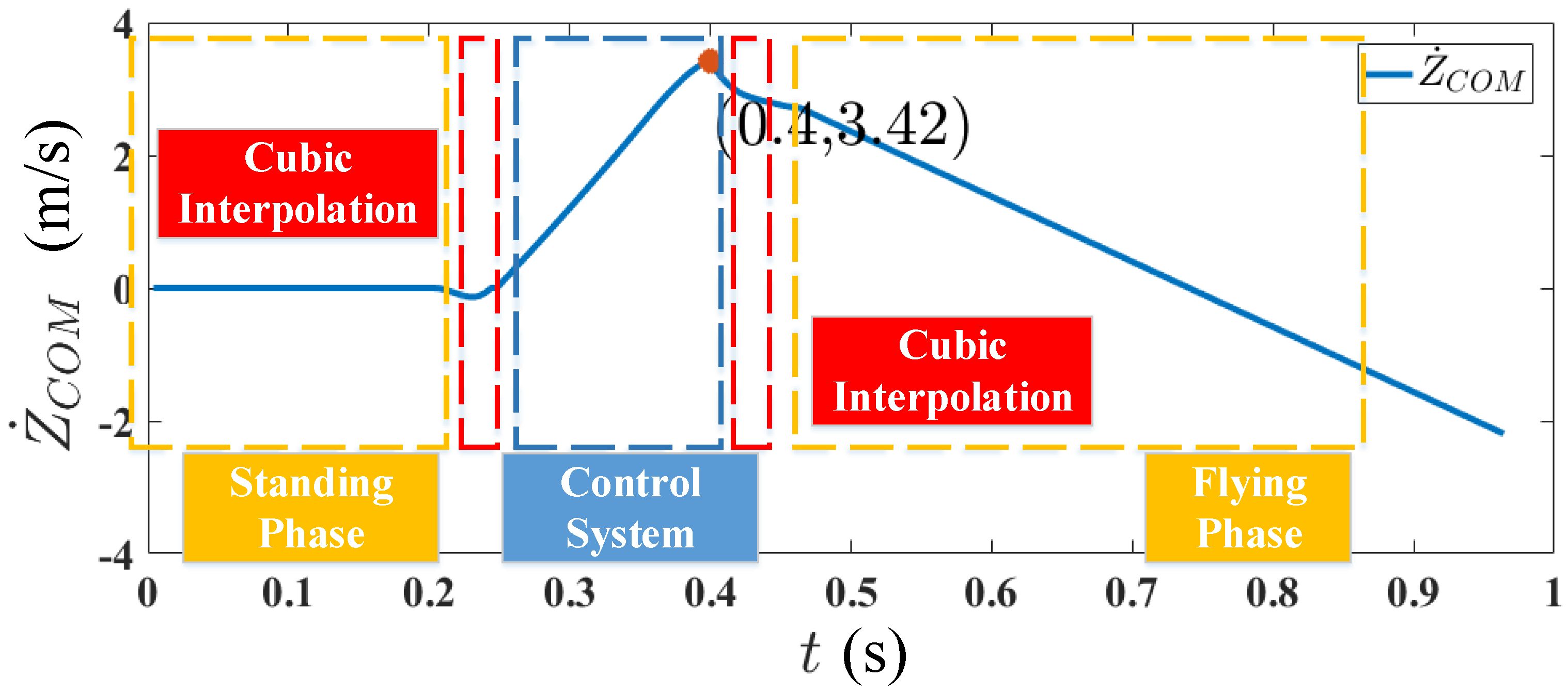
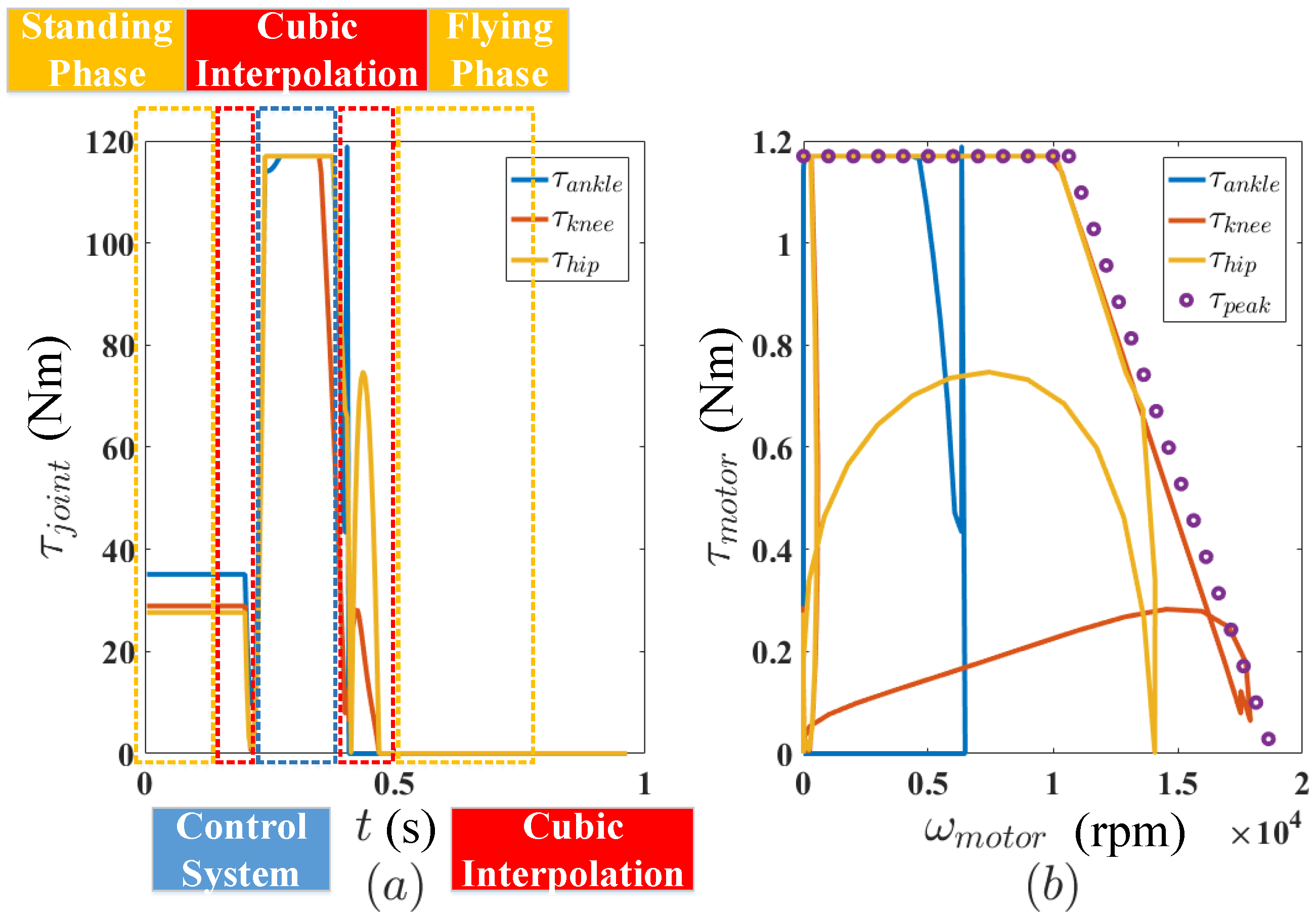
To verify our control method, we built a simplified model with the parameters in Table 1 in V-rep, a virtual robot experimentation platform. In the simulator, the model is controlled in position mode. In Figure 8, when the robot is going to take off, the jumping controller will not generate data any more, and the angles will be the same as the angles at the take-off time, and each joint will brake suddenly. Since the values of joint angular velocity and angular acceleration are large at the take-off time. If we don’t smooth the joint trajectory after take-off, the motor will violate the torque constraint. Thus, we use the cubic interpolation in a joint trajectory to help the joint brake smoothly. The cubic interpolation is also used to smooth the joint trajectory at the beginning of the jump, and the initial state changes from $X_0=(-{57}^{\circ },{158}^{\circ },-{126}^{\circ },0,0,0)$ to $X_0=(-{61.5}^{\circ },{155.2}^{\circ },-{123.8}^{\circ },0,0,0)$. Figure 12 shows the joint trajectory during simulation. By using playback of this offline pattern, we get the velocity of COM as shown in Figure 13. At $t=0.40$ (s), the translational velocity of COM in vertical direction reaches a maximum $3.42$ (m/s). Without consideration of the influence of the added trajectory near the taking off time, the jump height is about $0.596$ (m), which can be calculated by Equation (12). The added trajectory leads to the slight decrease in vertical velocity at the take-off time, which is a little delayed. From the simulation, we got the position of the foot and COM in vertical direction and the torque of each joint as shown in Figure 14 and Figure 15. If we take the distance between foot and ground as the jump height, then the maximal jump height is about $0.477$ (m) and the COM is increased by $0.83$ (m). During the entire motion, the joint torque profiles are within the profile of the motor torque speed curve. Finally, the jumping motion sequence is shown in Figure 16.

5. Conclusions

This paper proposes a motion planning method to allow a bipedal robot to perform a jumping maneuver. It proves the possibility for bipedal robot driven by electric motors to perform a high jump. Using a simplified model without any elastic elements, we greatly increased the jumping height by commanding every motor as much as possible to yield the profile of the torque speed curve, which reflects the obstacle negotiation capability. During the push-off phase, linear programming is used to fine-tune the joint torques to ensure that the torque and ZMP constraints are satisfied. Finally, in simulations, the robot successfully jumped 0.477 (m) high, and the COM is increased by 0.83 (m). However, some limitations should be noted.

• In this paper, the efficiency of harmonic reducer is not considered. Thus, we have to calibrate the torque speed curve of the motor on a professional motor test platform, with and without reducer.
• While we can obtain an increased jump height based on the premise of the torque and ZMP constraints, how to reduce the impact force and maintain landing equilibrium during the landing phase remains a significant problem.
• We only found that the jump direction $\theta$ and the initial ankle angle $q_{10}$ have an almost linear relationship. However, this relationship alone is not sufficiently reliable to specify jumping direction.

In the future, we will take the efficiency of harmonic reducer, flying and landing phase of jump into consideration. Future work should include development of a sequential jumping motion and a running motion to provide further improvements in the obstacle negotiation abilities of the bipedal robot. It is also necessary to design experiments to validate the theory in the future.

References

- Huang, Q.; Yokoi, K.; Kajita, S.; Kaneko, K.; Arai, H.; Koyachi, N.; Tanie, K. Planning walking patterns for a biped robot. IEEE Trans. Robot. Autom. 2001, 17, 280–289. [Google Scholar] [CrossRef]
- Huang, Q.; Kajita, S.; Koyachi, N.; Kaneko, K.; Yokoi, K.; Arai, H.; Komoriya, K.; Tanie, K. A high stability, smooth walking pattern for a biped robot. In Proceedings of the 1999 IEEE International Conference on Robotics and Automation, Detroit, MI, USA, 10–15 May 1999; Volume 1, pp. 65–71. [Google Scholar]
- Li, C.; Lowe, R.; Duran, B.; Ziemke, T. Humanoids that crawl: comparing gait performance of iCub and NAO using a CPG architecture. In Proceedings of the 2011 IEEE International Conference on Computer Science and Automation Engineering (CSAE), Shanghai, China, 10–12 June 2011; Volume 4, pp. 577–582. [Google Scholar]
- Kuehn, D.; Bernhard, F.; Burchardt, A.; Schilling, M.; Stark, T.; Zenzes, M.; Kirchner, F. Distributed computation in a quadrupedal robotic system. Int. J. Adv. Robotic. Syst. 2014, 11, 110. [Google Scholar] [CrossRef]
- Fujiwara, K.; Kanehiro, F.; Kajita, S.; Kaneko, K.; Yokoi, K.; Hirukawa, H. Falling motion control to minimize damage to biped humanoid robot. In Proceedings of the Conference on Intelligent Robots and Systems, Lausanne, Switzerland, 30 September–4 October 2002. [Google Scholar]
- Fujiwara, K.; Kajita, S.; Harada, K.; Kaneko, K.; Morisawa, M.; Kanehiro, F.; Nakaoka, S.; Hirukawa, H. Towards an optimal falling motion for a humanoid robot. In Proceedings of the 6th IEEE-RAS International Conference on Humanoid Robots, Genova, Italy, 4–6 December 2006; pp. 524–529. [Google Scholar]
- Kajita, S.; Nagasaki, T.; Kaneko, K.; Yokoi, K.; Tanie, K. A hop towards running humanoid biped. In Proceedings of the IEEE International Conference on Robotics and Automation, New Orleans, LA, USA, 26 April–1 May 2004; Volume 1, pp. 629–635. [Google Scholar]
- Sakka, S.; Yokoi, K. Humanoid vertical jumping based on force feedback and inertial forces optimization. In Proceedings of the IEEE International Conference on Robotics and Automation, Barcelona, Spain, 18–22 April 2005; pp. 3752–3757. [Google Scholar]
- Curran, S.; Orin, D.E. Evolution of a jump in an articulated leg with series-elastic actuation. In Proceedings of the IEEE International Conference on Robotics and Automation, Pasadena, CA, USA, 19–23 May 2008; pp. 352–358. [Google Scholar]
- Raibert, M.H.; Brown, H.B., Jr.; Chepponis, M. Experiments in balance with a 3D one-legged hopping machine. Int. J. Robot. Res. 1984, 3, 75–92. [Google Scholar] [CrossRef]
- Chen, X.; Zhangguo, Y.; Zhang, W.; Zheng, Y.; Huang, Q.; Ming, A. Bio-inspired Control of Walking with Toe-off, Heel-strike and Disturbance Rejection for a Biped Robot. IEEE Trans. Ind. Electron. 2017, 64, 7962–7971. [Google Scholar] [CrossRef]
- Yu, D.; Yu, Z.; Fang, X.; Lei, S.; Chen, X.; Huang, Q.; Meng, L.; Zhou, Q.; Zhang, W.; Han, J. Rolling motion generation of multi-points contact for a humanoid robot. In Proceedings of the International Conference on Advanced Robotics and Mechatronics (ICARM), Macau, China, 18–20 August 2016; pp. 153–158. [Google Scholar]
- Li, Q.; Chen, X.; Zhou, Y.; Yu, Z.; Zhang, W.; Huang, Q. A minimized falling damage method for humanoid robots. Int. J. Adv. Robot. Syst. 2017, 14, 1729881417728016. [Google Scholar] [CrossRef]
- Raibert, M.H. Legged Robots That Balance; MIT Press: Cambridge, MA, USA, 1986. [Google Scholar]
- Playter, R.R.; Raibert, M.H. Control of a Biped Somersault in 3D. In Proceedings of the IEEE/RSJ International Conference on Intelligent Robots and Systems, Raleigh, NC, USA, 7–10 July 1992; Volume 1, pp. 582–589. [Google Scholar]
- Vanderborght, B.; Van Ham, R.; Verrelst, B.; Van Damme, M.; Lefeber, D. Overview of the lucy project: Dynamic stabilization of a biped powered by pneumatic artificial muscles. Adv. Robot. 2008, 22, 1027–1051. [Google Scholar] [CrossRef]
- Hosoda, K.; Takuma, T.; Nakamoto, A.; Hayashi, S. Biped robot design powered by antagonistic pneumatic actuators for multi-modal locomotion. Robot. Autonom. Syst. 2008, 56, 46–53. [Google Scholar] [CrossRef]
- Ugurlu, B.; Saglia, J.A.; Tsagarakis, N.G.; Caldwell, D.G. Hopping at the resonance frequency: A trajectory generation technique for bipedal robots with elastic joints. In Proceedings of the IEEE International Conference on Robotics and Automation, Saint Paul, MN, USA, 14–18 May 2012; pp. 1436–1443. [Google Scholar]
- Okada, M.; Takeda, Y. Optimal design of nonlinear profile of gear ratio using non-circular gear for jumping robot. In Proceedings of the IEEE International Conference on Robotics and Automation, Saint Paul, MN, USA, 14–18 May 2012; pp. 1958–1963. [Google Scholar]
- Hondo, T.; Kinase, Y.; Mizuuchi, I. Jumping motion experiments on a NAO robot with elastic devices. In Proceedings of the 12th IEEE-RAS International Conference on Humanoid Robots (Humanoids), Osaka, Japan, 29 November–1 December 2012; pp. 823–828. [Google Scholar]
- Guizzo, E. Japanese Humanoid Robot Can Keep Its Balance After Getting Kicked. Available online: https://0-spectrum-ieee-org.brum.beds.ac.uk/automaton/robotics/humanoids/japanese-high-power-humanoid-robot-hrp3l-jsk/ (accessed on 8 May 2012).
- Nunez, V.; Drakunov, S.; Nadjar-Gauthier, N.; Cadiou, J. Control strategy for planar vertical jump. In Proceedings of the 12th International Conference on Advanced Robotics, Seattle, WA, USA, 18–20 July 2005; pp. 849–855. [Google Scholar]
- Ugurlu, B.; Kawamura, A. Real-time running and jumping pattern generation for bipedal robots based on ZMP and Euler’s equations. In Proceedings of the IEEE/RSJ International Conference on Intelligent Robots and Systems, St. Louis, MO, USA, 10–15 October 2009; pp. 1100–1105. [Google Scholar]
- Kajita, S.; Hirukawa, H.; Harada, K.; Yokoi, K. Introduction to Humanoid Robotics; Springer: Berlin, Germany, 2014; Volume 101. [Google Scholar]
- Hong, Y.D.; Lee, B. Evolutionary Optimization for Optimal Hopping of Humanoid Robots. IEEE Trans. Ind. Electron. 2017, 64, 1279–1283. [Google Scholar] [CrossRef]
- Takahide Yoshiike, M.K.; Ujino, R. Development of Experimental Legged Robot for Inspection and Disaster Response in Plants. In Proceedings of the IEEE International Conference on Intelligent Robots and Systems (IROS), Vancouver, BC, Canada, 24–28 September 2017; pp. 4869–4876. [Google Scholar]
Figure 1.
(a) BHR6 humanoid robot; (b) the simplified model with the similar physical properties of BHR6.
Figure 2.
The joint constraint for appropriate reduction ratio selection.
Figure 3.
Torque speed curve of the motor K044100-6Y-4.98Ams when the voltage supplied to the motor is 120 V.
Figure 4.
The control system for choosing an appropriate reduction radio for motor K044100-6Y-4.98Ams.
Figure 5.
With the same motor and model, different reduction ratio leads to different jump height. When the same initial state = (, , 0, 0, 0) is determined, the relationship between h and can be presented.
Figure 6.
All three joints are equipped with the same K044100-6Y-4.98Ams motor and the same reduction ratio of . (a) shows the torque of each joint; and (b) represents relationships between the motor torque and speed.
Figure 7.
(a) the ZMP (zero moment point) limitation in the y-direction (m); (b) the added to to maintain the ZMP constraint.
Figure 8.
The joint constraint is removed. The torque constraint is used to ensure that all three joint torques yield the torque speed curve profile. Furthermore, the ZMP constraint is used to keep the dynamic balance throughout the entire puss-off phase.
Figure 9.
(a) optimal knee angle for various initial values of ankle angle ; (b) optimal hip angle for various initial values of ankle angle ; (c) maximum jump height h for various initial values of ankle angle ; (d) jump direction for various initial values of ankle angle .
Figure 10.
Assuming that , (a) shows the torque of each joint; and (b) represents relationships between the motor torque and speed. At the beginning of the jump motion, the ankle joint torque is slightly reduced to satisfy the ZMP constraint. Similar effectiveness can also be observed when the robot is about to take off.
Figure 11.
Assuming that , the ZMP is limited by the ZMP constraint to maintain balance throughout the push-off phase.
Figure 12.
The trajectory of each joint during the simulation.
Figure 13.
The velocity of COM (center of mass) during the simulation.
Figure 14.
The foot and COM (center of mass) position in vertical direction in the simulation.
Figure 15.
(a) shows the torque of each joint in the simulation; and (b) represents relationships between the motor torque and speed in the simulation.
Figure 16.
Screenshot of the simulation.