GARLM: Greedy Autocorrelation Retrieval Levenberg–Marquardt Algorithm for Improving Sparse Phase Retrieval

Abstract

The goal of phase retrieval is to recover an unknown signal from the random measurements consisting of the magnitude of its Fourier transform. Due to the loss of the phase information, phase retrieval is considered as an ill-posed problem. Conventional greedy algorithms, e.g., greedy spare phase retrieval (GESPAR), were developed to solve this problem by using prior knowledge of the unknown signal. However, due to the defect of the Gauss–Newton method in the local convergence problem, especially when the residual is large, it is very difficult to use this method in GESPAR to efficiently solve the non-convex optimization problem. In order to improve the performance of the greedy algorithm, we propose an improved phase retrieval algorithm, which is called the greedy autocorrelation retrieval Levenberg–Marquardt (GARLM) algorithm. Specifically, the proposed GARLM algorithm is a local search iterative algorithm to recover the sparse signal from its Fourier transform magnitude. The proposed algorithm is preferred to existing greedy methods of phase retrieval, since at each iteration the problem of minimizing the objective function over a given support is solved by using the improved Levenberg–Marquardt (ILM) method and matrix transform. A local search procedure such as the 2-opt method is then invoked to get the optimal estimation. Simulation results are given to show that the proposed algorithm performs better than the conventional GESPAR algorithm.

1. Introduction

In recent years, sampling theory has made significant progress [1], which has a great impact on signal processing and communication. More and more scholars ignore Nyquist’s sampling law and use a series of filtering operations to accurately recover the signal from its linear sample.

As we know, Fourier analysis and wavelet analysis are essential for these signal processing techniques, and the mathematical tools involving Fourier and wavelet analysis for sampling and reconstruction are very important [2,3]. Reference [2] used Riesz bases and frames to study stable reconstructions and generalize the concept of oblique double frames to the infinite-dimensional framework. The authors of Reference [3] developed a redundant sampling procedure that can be used to reduce quantization errors when quantizing measurements before reconstruction.

Concerning reconstruction techniques taking advantage of sparsity in general, the basic work of processing noise measurements and non-ideal sampling is an important part of recovering unknown signals from random measurements [4,5]. The problem of linear reconstruction based on Fourier analysis has also been recently considered [6,7,8,9]. For signal reconstruction techniques that are not based on sparsity assumptions, the random interpolation of linear interpolation can solve this problem. The first attempt to stochastically characterize the sampling via point process (PP) was done in Reference [10], where sample positions are the outcome of a Poisson PP (independently scattered points). Extensions of such a result to the multidimensional domain can be found in References [11,12,13] for homogeneous and inhomogeneous sampling with uncertainties, while PPs taking stochastic repulsion/attraction into account (i.e., the Ginibre PP and the Gauss–Poisson PP) have been recently considered [14,15]. In addition, the machine learning approach based on Gaussian random processes can also be used to solve signal reconstruction problems [16,17,18,19].

In this paper, the method we use to reconstruct the signal is phase retrieval. Phase retrieval is a typical signal reconstruction problem which seeks to recover a signal or image from the magnitude of linear measurements [20]. This problem occurs in many application areas, such as crystallography [21], optical imaging [22], waveform optimization [23], and other areas [24,25,26]. In general, because of the loss of Fourier phase information, the problem of phase retrieval is ill-posed and non-convex. The existing approach to address this problem involves exploiting prior knowledge of the signal domain [27,28,29,30]. Here we focus on the recovery of one-dimensional sparse signals from their Fourier measurements, which has been emphasized in recent works. The most popular method for phase retrieval is based on the use of alternating projections between the different constraints in time and the Fourier magnitude constraints [31,32,33], pioneered by Gerchberg and Saxton, and later extended by Fienup. The Gerchberg and Saxton (GS) algorithm in [32] uses image amplitude and Fourier transform spectral amplitude as a priori information to reconstruct the image by alternately applying amplitude constraints in the object and frequency domains. However, the GS algorithm converges slowly and is prone to stagnation. Fienup et al. have improved the GS algorithm and proposed the addition of error reduction (ER) and hybrid input–output (HIO) [31]. ER and HIO algorithms are used to determine the image pixel estimation value obtained in the object domain by iteratively alternating projection in the object domain and the frequency domain, setting the pixel value that does not satisfy the constraint to zero, and replacing the image Fourier amplitude with the measured value in the frequency domain.

Another state-of-the-art method uses the semi-definite programming (SDP) technique and low-rank matrix recovery framework [34,35,36]. Candes et al. proposed the PhaseLift algorithm [36], which involves lifting the phase retrieval problem that satisfies the non-convex constraint, and directly transforming this problem into solving the Hermitian matrix with rank one, achieving the transformation from non-convex constraints to convex constraints. However, because of the matrix lifting procedure, these SDP algorithms are unsuitable for large-scale signal recovery problems. These algorithms are simple, and it is easy to obtain a local minimum solution.

In recent years, many researchers have begun to explore the relationship between phase retrieval and structural information processing, such as applying the sparse representation of image structures to phase retrieval problems [37,38]. Sparse representation is one of the core research issues of compression sensing. It utilizes a linear combination of a small number of elements to describe the signal in some bases or dictionaries, simplifying the representation of complex signals [39,40]. Hence it is widely used in multiple image processing fields [41,42,43]. More recently, several robust phase recovery algorithms combating Gaussian noise have been proposed for targeting the noise in the measured values. For example, a fast local search method called greedy sparse phase retrieval (GESPAR) [44] is used. This is based on a fast 2-opt local search method with the known sparsity priors, and by iteratively updating the support of the underlying signal, the damped Gauss–Newton method is used to estimate the local minimum of the objective function. However, this algorithm cannot be used efficiently due to the defect of the Gauss–Newton method in the local convergence problem, especially when the residual is large.

In order to improve the calculation efficiency, this paper proposes an improved efficient local alternative search algorithm for sparse phase retrieval. First, the phase retrieval problem is formulated as an optimization, in terms of minimizing the sum of squared errors with support information. We then use proprietary techniques to estimate the signal, using a continuous optimization algorithm to ensure convergence to the critical point. Compared with the existing methods, our method—referred to as greedy autocorrelation retrieval Levenberg–Marquardt (GARLM)—is easy to implement and can recover signals more effectively.

The rest of the paper is organized as follows: the formulation of the phase retrieval and the support information is discussed in Section 2. In Section 3, after a brief overview of the general Levenberg–Marquardt (LM) method and 2-opt method, we describe our proposed algorithm in detail. Simulation results are presented in Section 4, and conclusions are drawn in Section 5.

2. Problem Formulation

In the phase retrieval problem, we consider an estimation problem of a $N$-dimensional complex signal vector $\mathit{x}$ from $M$ magnitude-squared linear measurements $\mathit{y}$. A basic phase retrieval model with Fourier measurements is related as:

$$y_i={\left|{{\displaystyle \sum }}_{n=0}^{N-1}{x}_n{e}^{-\frac{2\pi j\left(n-1\right)\left(i-1\right)}{M}}\right|}^2,i=1,\cdots ,M.$$

(1)

This formulation (Equation (1)) is equivalent to the matrix-vector multiplication $y_i={\left|F_i\mathit{x}\right|}^2$, where ${|·|}^2$ denotes the element-wise absolute squared value, $F\in {ℂ}^{N\times N}$ denotes the discrete Fourier transform (DFT) matrix with elements ${\varphi }^{\left(n-1\right)\left(i-1\right)}={\left(e^{-2\pi j/M}\right)}^{\left(n-1\right)\left(i-1\right)}$, and $F_i$ is the $i$th row of $F$. Here the signal $\mathit{x}$ is known to be sparse, and the measurements $y_i$ are known. To recover the signal $\mathit{x}$ with known sparsity level $s$ from the given measurements $y_i$, we consider a minimizing the sum of squared errors cost as:

$$\underset{\mathit{x}}{\min }{{\displaystyle \sum }}_{i=0}^{N-1}{({\left|F_i\mathit{x}\right|}^2-y_i)}^{2}s.t.{\Vert \mathit{x}\Vert }_0\le s.$$

(2)

The matrix-vector multiplication $F_i\mathit{x}$ is the fast Fourier transform (FFT), which can be written in terms of the autocorrelation function, i.e.,

$$\begin{array}{ll}{\left|F_i\mathit{x}\right|}^2& ={\displaystyle \sum }_{n=0}^N{\varphi }^{\left(n-1\right)\left(i-1\right)}{x}_n{\displaystyle \sum }_{v=0}^N{\varphi }^{-\left(v-1\right)\left(i-1\right)}{x}_v^{*}\\ & ={{\displaystyle \sum }}_{n=0}^N{{\displaystyle \sum }}_{v=0}^N{x}_n{x}_v^{*}{\varphi }^{\left(n-v\right)\left(i-1\right)}\\ & ={{\displaystyle \sum }}_{k=-N}^N{\varphi }^{km}{{\displaystyle \sum }}_{n=\max \left(k,0\right)}^{\min \left(N+k,N\right)}{x}_n{x}_{n-k}^{*}\\ & ={{\displaystyle \sum }}_{k=-N}^N{\varphi }^{km}{g}_k,\end{array}$$

(3)

where $g_k={\displaystyle \sum }_{n=\max \left(k,0\right)}^{\min \left(N+k,N\right)}{x}_n{x}_{n-k}^{*},k=N,\cdots ,-1,0,1,\cdots ,N$ is the autocorrelation sequence of $\mathit{x}$, and obviously $g_k$ can be obtained by the inverse DFT of $\mathit{y}$. Here, referring to GESPAR [44], we assume that no support cancelations occur in $g_k$, then we divide the support of the signal $\mathit{x}$ into two parts: $S_1$ and $S_2$. $S_1$ denotes the known indices in the support, and $S_2$ is the unknown indices in the off-support.

With these notations, defining $A_i=\Re {\left(F_i\right)}^T\Re \left(F_i\right)+\Im {\left(F_i\right)}^T\Im \left(F_i\right)$, Equation (2) can be rewritten as:

$$\begin{array}{l}\underset{x}{\min }f\left(\mathit{x}\right)\equiv {\displaystyle \sum }_{i=0}^{N-1}{\left({\mathit{x}}^T{A}_i\mathit{x}-y_i\right)}^2,\\ s.t.{\Vert \mathit{x}\Vert }_0\le s,\\ S_1\subseteq supp\left(\mathit{x}\right)\subseteq S_2,\end{array}$$

(4)

which will be the studied formulation in the next section.

3. Greedy Autocorrelation Retrieval Levenberg–Marquardt Algorithm

In this section, we briefly describe how to directly use existing methods to design a new algorithm called GARLM that solves Formulation (4) with high efficiency.

3.1. The Improved Levenberg–Marquardt Method

We first invoked an improved Levenberg–Marquardt (ILM) [45] method under the framework of gradient. Compared to the damped Gauss–Newton (DGN) method in [44], an ILM algorithm can guarantee that the iterative process always decreases when convergence is slow, and it can also ensure that the iterative process converges quickly in the neighborhood of the solution.

Similar to the DGN method, the ILM method is a common algorithm for solving nonlinear optimal problems, and it can only handle quadratic functions like Formulation (4). In order to avoid the latter algorithm being trapped into a local optimal solution when invoking the ILM algorithm, we rewarded a weight parameter ${\lambda }_i$ for $f\left(\mathit{x}\right)$, and the simulation results show that this effectively reduced the possibility of getting into a local optimal solution. The weight ${\lambda }_i$ is 1 or 3 with equal probability. We can invoke the ILM algorithm to solve the minimizing objective function $f\left(\mathit{x}\right)$, i.e.,

$$\begin{array}{l}f\left(\mathit{x}\right)={{\displaystyle \sum }}_{i=1}^N{\lambda }_i{\left(y_i-{\mathit{x}}^T{A}_i\mathit{x}\right)}^2={{\displaystyle \sum }}_{i=1}^N{\left(\sqrt{{\lambda }_i}\left(y_i-{\mathit{x}}^T{A}_i\mathit{x}\right)\right)}^2,\\ s.t.{\Vert \mathit{x}\Vert }_0\le s,\\ S_1\subseteq S\subseteq S_2.\end{array}$$

(5)

Here we denote $\mathit{z}$ to be a signal vector consisting of non-zero elements of $\mathit{x}$. Given the sparsity level $s$ of signal $\mathit{x}$, we can get $\mathit{z}\in {ℝ}^s$ corresponding to $\mathit{x}=I_s\mathit{z}$, where the matrix $I_s\in {ℝ}^{\mathit{N}\times \mathit{s}}$ is the $s$ columns of the identity matrix. Therefore Formulation (5) can be written as:

$$\begin{array}{ll}\mathrm{h}\left(\mathit{z}\right)& ={{\displaystyle \sum }}_{i=1}^N{\left(\sqrt{{\lambda }_i}(y_i-{(I_s\mathit{z})}^T{A}_i{I}_s\mathit{z})\right)}^2\\ & ={{\displaystyle \sum }}_{i=1}^N{\left(\sqrt{{\lambda }_i}(y_i-{\mathit{z}}^T{I}_s^T{A}_i{I}_s\mathit{z})\right)}^2\\ & ={{\displaystyle \sum }}_{i=1}^N{\left(\sqrt{{\lambda }_i}(y_i-{\mathit{z}}^T{B}_i\mathit{z})\right)}^2\\ & ={\displaystyle \sum }_{i=1}^N{p}_i^2\left(\mathit{z}\right),\end{array}$$

(6)

where $B_i=I_s^T{A}_i{I}_s$, and and $p_i\left(\mathit{z}\right)=\sqrt{{\lambda }_i}\left(y_i-{\mathit{z}}^T{B}_i\mathit{z}\right)$. At each iteration of ILM, we expand and approximate the first order Taylor of $p_i\left(\mathit{z}\right)$ around ${\mathit{z}}_k$ as:

$$p_i\approx p_i\left({\mathit{z}}_k\right)+\nabla p_i{\left({\mathit{z}}_k\right)}^T\left(\mathit{z}-{\mathit{z}}_k\right),$$

(7)

which is a linear least squares problem. Then via the ILM method we can get the solution to Formulation (7):

$${\mathit{z}}_{k+1}={\mathit{z}}_k+d_k={\mathit{z}}_k-{\left(2J{\left({\mathit{z}}_k\right)}^{T}J\left({\mathit{z}}_k\right)+\mu I\right)}^{-1}2J{\left({\mathit{z}}_k\right)}^T{p}_i,$$

(8)

where the element of the Jacobian matrix $J\left({\mathit{z}}_k\right)$ is $J_{ij}=\partial p_i/\partial {\mathit{z}}_j$, which means the $i$th row of $J\left({\mathit{z}}_k\right)$ is $\nabla p_i{\left({\mathit{z}}_k\right)}^T=2{\left(B_i{\mathit{z}}_k\right)}^T$, and the matrix $I\in {ℝ}^{\mathit{s}\times \mathit{s}}$ is an identity matrix. At each iteration, $p_i$ can be computed efficiently via FFT of $\mathit{x}$, which can also be used in the calculation of $J\left({\mathit{z}}_k\right)$. The step-size in Equation (8) is:

$$d_k=-{\left(2J{\left({\mathit{z}}_k\right)}^{T}J\left({\mathit{z}}_k\right)+\mu I\right)}^{-1}2J{\left({\mathit{z}}_k\right)}^T{p}_i,$$

(9)

where the damping term $\mu$ is chosen via the trust region method [46], which is an important technique in the optimization algorithm to ensure global convergence. To ensure $\mu$, first we must ensure the gain ratio $q$ which is given by:

$$q=∆h_k/∆L_k=\frac{\left(\mathrm{h}\left({\mathit{z}}_k\right)-\mathrm{h}\left({\mathit{z}}_k+d_k\right)\right)}{\left(\frac{1}{2}{\left(d_k\right)}^T\left(\mu d_k-J{\left({\mathit{z}}_k\right)}^T{p}_i\right)\right)},$$

where $∆h_k=\mathrm{h}\left({\mathit{z}}_k\right)-\mathrm{h}\left({\mathit{z}}_k+d_k\right)$ is the actual decrease of $h$ at the $k$th iteration, and $∆L_k=L\left(0\right)-L\left(d_k\right)$ means the predicted decline of $h$, and $L\left(d_k\right)$ is the approximate function of $h$. If $q$ is large, indicating that $L\left(d_k\right)$ is very close to $\mathrm{h}\left({\mathit{z}}_k+d_k\right)$, we can reduce the damping term μ so that the algorithm is closer to the Gauss–Newton algorithm at the next iteration. If $q$ is small or negative, it means poor approximation. We need to increase $\mu$ and reduce the step-size, so that the algorithm is closer to the gradient descent method. Algorithm 1 describes the ILM method in detail. We choose the initial point ${\mathit{z}}_0$ as a white random Gaussian vector with zero mean and unit variance, the initial damping term $\mu =1$, the stopping parameter $\mathsf{\xi }={10}^{-6}$, and the maximum allowed iterations $L=100$.

Algorithm 1. ILM Algorithm.

Input: Symmetric matrices $A_i$, and measurement $y_i$, the given indices set $S$, the maximum number of iterations $L$, and the stopping threshold $\mathsf{\xi }$. Output: The optimal estimate of sparse signal x of (5). Generate an initial vector ${\mathit{x}}_0$ with the given support S, then we have ${\mathit{z}}_0={\mathit{x}}_0\left(S\right)$, the initial damping term $\mathsf{\mu }=1$, and the initial parameter $\mathrm{v}=2$. For $k=0,1,\cdots ,L$ do The solution of the linear least squares problem (6) is ${\mathit{z}}_{k+1}={\mathit{z}}_k-{\left(2J{\left({\mathit{z}}_k\right)}^{T}J\left({\mathit{z}}_k\right)+\mu I\right)}^{-1}2J{\left({\mathit{z}}_k\right)}^T$, the $i$th row of $J\left({\mathit{z}}_k\right)$ is $\nabla p_i{\left({\mathit{z}}_k\right)}^T=2{\left(B_i{\mathit{z}}_k\right)}^T$, and the damping term $\mu$ is determined by $q$. The gain ratio $q=\left(\mathrm{h}\left({\mathit{z}}_k\right)-\mathrm{h}\left({\mathit{z}}_k+d_k\right)\right)/\left(0.5\ast {\left(d_k\right)}^T\left(\mu d_k-J{\left({\mathit{z}}_k\right)}^T{p}_i\right)\right)$ if $q>0$ v=2; ${\mathit{z}}_k={\mathit{z}}_{k+1};\mu =\mu \ast \max \left\{1/3,1-{\left(2q-1\right)}^3\right\}$ else $\mu =\mu \ast \mathrm{v}$; $\mathrm{v}=2\mathrm{v}$. If $\parallel {\mathit{x}}_{k+1}-{\mathit{x}}_k\parallel <\mathsf{\xi }$, then stop the iteration, otherwise go to step 3. End for

3.2. 2-Opt Method of the Support Information

Similar to the GESPAR algorithm, our algorithm invokes a local search procedure, just like the 2-opt method. First, we have an initial random support set $S$ of the signal $\mathit{x}$, and $S$ satisfies the support constraints $S_1\subseteq S\subseteq S_2$. Then, the two indices $i$ in $S_1$ and $j$ in $S_2$ are exchanged to get a new support $S^{\prime }$. The swapped index $i$ in $S_1$ corresponds to the current iterate value ${\min }_i\left|{\mathit{x}}_k\right|$, and the swapped index $j$ in $S_2$ corresponds to ${\max }_j\nabla f\left({\mathit{x}}_k\right)$. After the exchange is completed, our algorithm will invoke the ILM algorithm with new support $S^{\prime }$ to get the optimal solution of Formulation (5). After the optimal value is output, it will be exchanged until the optimal solution is obtained. Algorithm 2 describes the 2-opt method in detail, and we set the total number of index replacements $T=6400$.

Algorithm 2. 2-Opt Algorithm.

Input: Symmetric matrices $A_i$, the measurement $y_i$, the stopping threshold $\tau$, and the maximum number of index exchanging T. Output: The optimal estimate of sparse signal $\mathit{x}$ for Formulation (5). Generate a random index set $S_0$, then invoke the ILM algorithm ${\mathit{x}}_0=\mathrm{ILM}\left[A_i,y_i,S_0,L,\mathsf{\xi }\right]$ For $k=1,2,\cdots$ do Let $i={\min }_i\left|{\mathit{x}}_k\right|$,$j={\max }_j\nabla f\left({\mathit{x}}_k\right)$, make an exchange between them to generate a new index set $S_k$. Invoke ILM algorithm ${\mathit{x}}_{k+1}=\mathrm{ILM}\left[{\mathit{w}}_i,y_i,S_k,L,\mathsf{\xi }\right]$ and advance T. If $f\left({\mathit{x}}_{k+1}\right)<f\left({\mathit{x}}_k\right)$, then advance k, otherwise continue to exchange up to T. Stop if $f\left({\mathit{x}}_{k+1}\right)<\tau$, and the output is ${\mathit{x}}_{k+1}$. End for

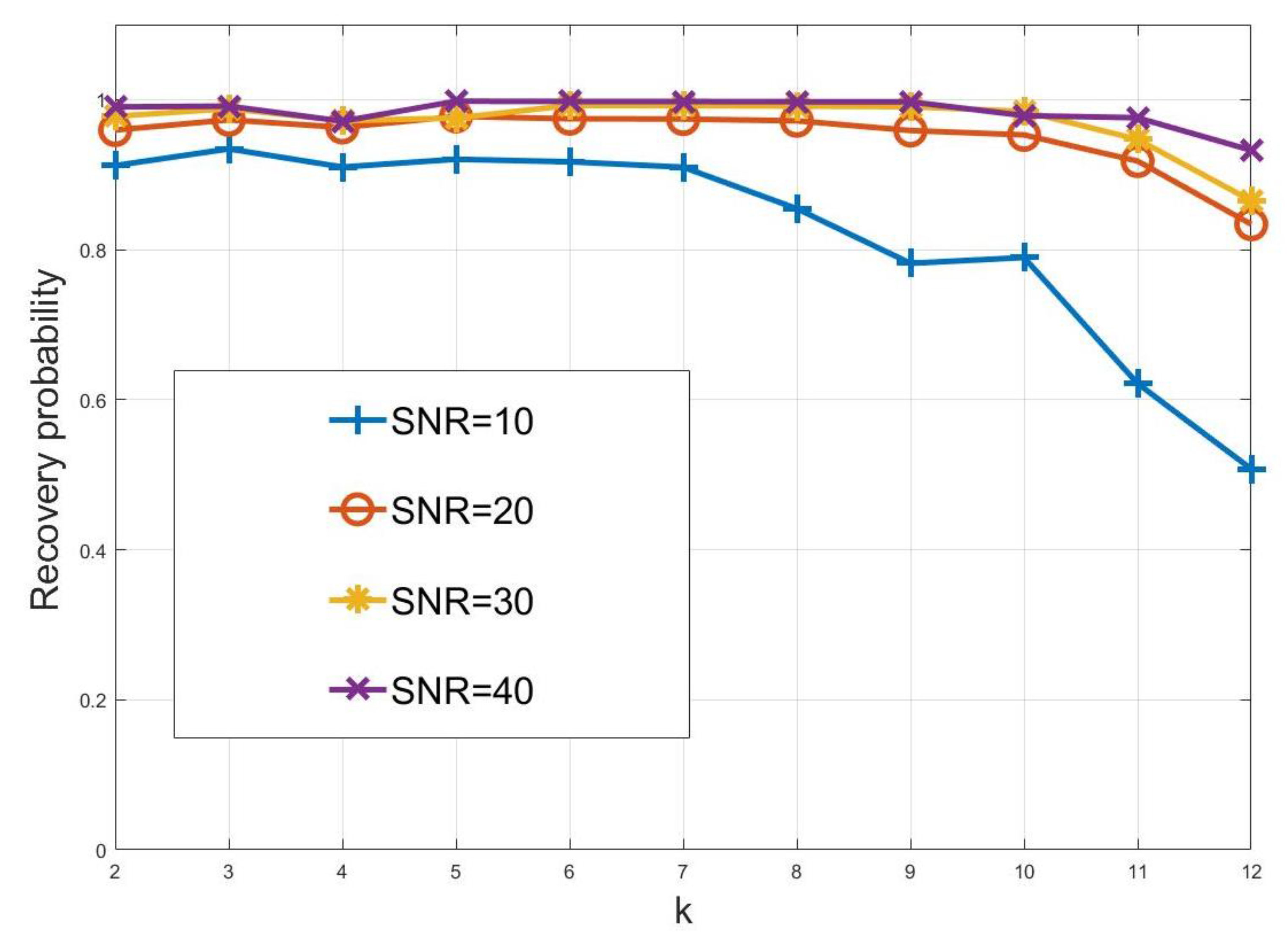
4. Simulation Results and Discussions

In this section we conducted some experimental simulations to investigate the performance of the proposed GARLM algorithm, comparing it to the typical greedy algorithm GESPAR in various situations, such as recovery probability, robustness to noise, and effectiveness.

We considered a random vector $\mathit{x}$ of length $n$ as the original unknown signal with randomly chosen elements, the sparsity level of this signal as $k$, and the magnitude square of its N-point DFT as $y$, as the sampling measurement. Our goal was to recover the unknown signal—which is known to be sparse—from the magnitude square of its Fourier transform. To achieve this target, we listed some important system parameters. The number of maximum indices in the index set $S$ is $n=64$ and the number of the sampling measurement $y_i$ is $N=128$, and the two algorithms both use $\tau ={10}^{-6}$ and $T=6400$ to recover the signal $\mathit{x}$. All the experiments were performed in MATLAB on a desk station with a two 2.3 GHz Intel Core i5 CPU and 4 GB of ROM.

We chose to use signal recovery probability to measure the effectiveness of different algorithms for signal recovery. The signal recovery probability was defined as the ratio of successful recovery signals in 100 simulations. Figure 1 shows the comparison of the effectiveness of the signal recovery probability of different algorithms, and the probability of successful recovery is shown by different sparsity levels. Here we compare the signal recovery probabilities of the GARLM and GESPAR algorithms at the same sparsity, and in each simulation both the original signal and its support are randomly reset. We observed that both the GARLM and GESPAR algorithms had a high successful recovery probability, the signal recovery probability was close to 100% before the signal sparsity level $k$ was less than or equal to 13, and the performance of GARLM was better because its successful recovery probability began to decline up to $k=16$. As the sparsity level $k$ continued to increase, we observed that the probability of successful recovery of the two algorithms decreased, but the performance of the GARLM algorithm was still obviously better than the GESPAR algorithm.

Although it was expected that our algorithm should outperform GESPAR in the measurement setup in a noise-free environment, in real life the measurements we get are always accompanied by noise, which degrades the performance of the algorithm. It is therefore necessary to consider the effectiveness of the algorithm in the presence of noise. We wanted to observe its normalized mean square error (NMSE) performances with different signal-to-noise ratio (SNR) values.

In our simulation, we still chose the random vector $\mathit{x}$ of length $n$ with randomly chosen elements as the original unknown signal, its sparsity level as $k$, and the magnitude square of its N-point DFT as $y$. We considered adding random white Gaussian noise $n$ to the measurements $y,y={\left|F\mathit{x}\right|}^2+n$. To recover the unknown signal, our algorithm GARLM chose $n=64,N=128,\tau ={10}^{-6},T=10000$, and SNR $=\left\{10,20,30,40\right\}$ dB, as well as GESPAR. Figure 2 shows the NMSE performances versus sparsity level $k$ at different SNR values—the NMSE defined as $\mathrm{NMSE}=\frac{{\Vert \mathit{x}-\widehat{\mathit{x}}\Vert }_2}{{\Vert \mathit{x}\Vert }_2}.$ We observed that when SNR = 10, the overall performance of the GARLM algorithm was better than the GESPAR algorithm. With the increase of sparsity $k$, the noise robustness of the GARLM algorithm was better than the GESPAR algorithm, except for $k=9$. This situation also occurred in other SNR values. We observed that as the SNR increases, the performance of our algorithm naturally increased, and it clearly performed better than GESPAR in terms of noise robustness under most SNR values.

Figure 3 shows the recovery probability under different channel sparsity levels under different SNR environments. We observed an almost 100% successful recovery with $\mathrm{SNR}>10$ before the sparsity $k=10$. The recovery probability at $\mathrm{SNR}=10$ also had a very high probability before the sparsity level $k<8$, which showed that the effectiveness of the algorithm is guaranteed even under low-SNR conditions. As the SNR increased, the effectiveness of the algorithm gradually increased. Hence Figure 3 implies that our proposed algorithm performed well under different SNRs.

5. Conclusions

In this paper, we proposed an improved and efficient local alternative search algorithm for phase retrieval named GARLM. Specifically, the proposed GARLM algorithm is a local search iterative algorithm to recover the sparse signal from its Fourier transform magnitude. The proposed algorithm is preferred to existing greedy methods of phase retrieval. The problem of phase retrieval is a non-convex problem of minimizing the sum of squared errors with support information. To recover the unknown signal, we first transformed this non-convex problem to a linear least squares problem, and then invoked ILM and 2-opt algorithms to recover the original signal. Simulation results have confirmed that compared to the classic greedy algorithm GESPAR for phase retrieval, our algorithm performs well in terms of recovery probability, robustness to noise, and effectiveness. The proposed algorithm GARLM has also proved to be effective in solving phase retrieval problems and performs well in terms of noise robustness via simulations.

References

1. O’Donnell, R. Sampling—50 Years After Shannon. Proc. IEEE 2000, 88, 567–568. [Google Scholar] [CrossRef]
2. Eldar, Y.C.; Werther, T. General Framework for Consistent Sampling in Hilbert Spaces. Int. J. Wavel. Multiresolut. Inf. Process. 2005, 3, 497–509. [Google Scholar] [CrossRef]
3. Eldar, Y.C. Sampling and reconstruction in arbitrary spaces and oblique dual frame vectors. J. Fourier Anal. Appl. 2003, 1, 77–96. [Google Scholar] [CrossRef]
4. Dvorkind, T.G.; Eldar, Y.C.; Matusiak, E. Nonlinear and nonideal sampling: Theory and methods. IEEE Trans. Signal Process. 2008, 56, 5874–5890. [Google Scholar] [CrossRef]
5. Eldar, Y.C.; Unser, M. Nonideal sampling and interpolation from noisy observations in shift-invariant spaces. IEEE Trans. Signal Process. 2006, 54, 2636–2651. [Google Scholar] [CrossRef] [Green Version]
6. Dardari, D.; Pasolini, G.; Zabini, F. An efficient method for physical fields mapping through crowdsensing. Pervasive Mob. Comput. 2018, 48, 69–83. [Google Scholar] [CrossRef]
7. Reise, G.; Matz, G.; Gröchenig, K. Distributed field reconstruction in wireless sensor networks based on hybrid shift-invariant spaces. IEEE Trans. Signal Process. 2012, 60, 5426–5439. [Google Scholar] [CrossRef]
8. Masry, E. Random sampling of deterministic signals: Statistical analysis of Fourier transform estimates. IEEE Trans. Signal Process. 2006, 54, 1750–1761. [Google Scholar] [CrossRef]
9. Tarczynski, A.; Allay, N. Spectral analysis of randomly sampled signals: Suppression of aliasing and sampler jitter. IEEE Trans. Signal Process. 2004, 52, 3324–3334. [Google Scholar] [CrossRef]
10. Marvasti, F.A. Signal Recovery from Nonuniform Samples and Spectral Analysis on Random Nonuniform Samples. In Proceedings of the IEEE International Conference on Acoustics, Speech, and Signal Processing (ICASSP), Tokyo, Japan, 7–11 April 1986; Volume 11, pp. 1649–1652. [Google Scholar]
11. Zabini, F.; Conti, A. Process estimation from randomly deployed wireless sensors with position uncertainty. In Proceedings of the 2011 IEEE Global Telecommunications Conference (GLOBECOM), Kathmandu, Nepal, 5–9 December 2011. [Google Scholar]
12. Zabini, F.; Conti, A. Inhomogeneous Poisson Sampling of Finite-Energy Signals with Uncertainties in Rd. IEEE Trans. Signal Process. 2016, 64, 4679–4694. [Google Scholar] [CrossRef]
13. Dardari, D.; Conti, A.; Buratti, C.; Verdone, R. Mathematical evaluation of environmental monitoring estimation error through energy-efficient wireless sensor networks. IEEE Trans. Mob. Comput. 2007, 6, 790–802. [Google Scholar] [CrossRef]
14. Zabini, F.; Conti, A. Ginibre sampling and signal reconstruction. In Proceedings of the 2016 IEEE International Symposium on Information Theory (ISIT), Barcelona, Spain, 10–15 July 2016; pp. 865–869. [Google Scholar]
15. Zabini, F.; Pasolini, G.; Conti, A. On random sampling with nodes attraction: The case of Gauss-Poisson process. In Proceedings of the 2017 IEEE International Symposium on Information Theory (ISIT), Aachen, Germany, 25–30 June 2017; pp. 2278–2282. [Google Scholar]
16. Särkkä, S.; Solin, A.; Hartikainen, J. Spatio-Temporal Learning via Infinite-Dimensional Bayesian Filtering and Smoothing. IEEE Signal Process. Mag. 2013, 30, 51–61. [Google Scholar] [CrossRef]
17. Xu, Y.; Choi, J. Spatial prediction with mobile sensor networks using Gaussian processes with built-in Gaussian Markov random fields. Automatica 2012, 48, 1735–1740. [Google Scholar] [CrossRef]
18. Krause, A.; Singh, A.; Guestrin, C. Near-Optimal Sensor Placements in Gaussian Processes: Theory, Efficient Algorithms and Empirical Studies. J. Mach. Learn. Res. 2008, 9, 235–284. [Google Scholar]
19. Krause, A.; Guestrin, C. Nonmyopic active learning of Gaussian processes: An exploration-exploitation approach. In Proceedings of the 24th International Conference on Machine Learning (ICML), Corvalis, OR, USA, 20–24 June 2007; pp. 449–456. [Google Scholar]
20. Hurt, N.E. Phase Retrieval and Zero Crossings: Mathematical Methods in Image Reconstruction; Springer Science & Business Media: New York, NY, USA, 2001; Volume 52. [Google Scholar]
21. Harrison, R.W. Phase problem in crystallography. J. Opt. Soc. Am. A 1993, 10, 1046–1055. [Google Scholar] [CrossRef]
22. Walther, A. The Question of Phase Retrieval in Optics. Opt. Acta Int. J. Opt. 1963, 10, 41–49. [Google Scholar] [CrossRef]
23. Patton, L.K.; Rigling, B.D. Phase retrieval for radar waveform optimization. IEEE Trans. Aerosp. Electron. Syst. 2012, 48, 3287–3302. [Google Scholar] [CrossRef]
24. Le Roux, J.; Vincent, E. Consistent Wiener Filtering for Audio Source Separation. IEEE Signal Process. Lett. 2013, 20, 217–220. [Google Scholar] [CrossRef] [Green Version]
25. Miao, J.; Ishikawa, T.; Johnson, B.; Anderson, E.H.; Lai, B.; Hodgson, K.O. High resolution 3D X-ray diffraction microscopy. Phys. Rev. Lett. 2002, 89, 088303. [Google Scholar] [CrossRef] [PubMed]
26. Sturmel, N.; Daudet, L. Signal reconstruction from STFT magnitude: A state of the art. In Proceedings of the 14th International Conference on Digital Audio Effects (DAFx’11), Paris, France, 19–23 September 2011; Volume 2012, pp. 375–386. [Google Scholar]
27. Ohlsson, H.; Eldar, Y.C. On conditions for uniqueness in sparse phase retrieval. In Proceedings of the 2014 IEEE International Conference on Acoustics, Speech and Signal Processing (ICASSP), Florence, Italy, 4–9 May 2014; pp. 1841–1845. [Google Scholar]
28. Jaganathan, K.; Oymak, S.; Hassibi, B. Recovery of sparse 1-D signals from the magnitudes of their Fourier transform. In Proceedings of the 2012 IEEE International Symposium on Information Theory, Cambridge, MA, USA, 1–6 July 2012; pp. 1473–1477. [Google Scholar]
29. Eldar, Y.C.; Mendelson, S. Phase retrieval: Stability and recovery guarantees. Appl. Comput. Harmon. Anal. 2014, 36, 473–494. [Google Scholar] [CrossRef] [Green Version]
30. Lu, Y.M.; Vetterli, M. Sparse spectral factorization: Unicity and reconstruction algorithms. In Proceedings of the 2011 IEEE International Conference on Acoustics, Speech and Signal Processing (ICASSP), Prague, Czech Republic, 22–27 May 2011; pp. 5976–5979. [Google Scholar]
31. Fienup, J.R.R. Phase retrieval algorithms: A comparison. Appl. Opt. 1982, 21, 2758–2769. [Google Scholar] [CrossRef] [PubMed]
32. Gerchberg, R.W.; Saxton, W.O. A practical algorithm for the determination of phase from image and diffraction plane pictures. Optik 1972, 35, 237–246. [Google Scholar]
33. Bauschke, H.H.; Combettes, P.L.; Luke, D.R. Phase retrieval, error reduction algorithm, and Fienup variants: A view from convex optimization. J. Opt. Soc. Am. A Opt. Image Sci. Vis. 2002, 19, 1334–1345. [Google Scholar] [CrossRef] [PubMed]
34. Shechtman, Y.; Eldar, Y.C.; Szameit, A.; Segev, M. Sparsity based sub-wavelength imaging with partially incoherent light via quadratic compressed sensing. Opt. Express 2011, 19, 14807–14822. [Google Scholar] [CrossRef] [PubMed]
35. Candes, E.J.; Eldar, Y.C.; Strohmer, T.; Voroninski, V. Phase retrieval via matrix completion. SIAM Rev. 2015, 57, 225–251. [Google Scholar] [CrossRef]
36. Candès, E.J.; Strohmer, T.; Voroninski, V. PhaseLift: Exact and stable signal recovery from magnitude measurements via convex programming. Commun. Pure Appl. Math. 2013, 66, 1241–1274. [Google Scholar] [CrossRef]
37. Wen, J.; Zhou, Z.; Wang, J.; Tang, X.; Mo, Q. A Sharp Condition for Exact Support Recovery with Orthogonal Matching Pursuit. IEEE Trans. Signal Process. 2017, 65, 1370–1382. [Google Scholar] [CrossRef]
38. Wen, J.; Li, D.; Zhu, F. Stable recovery of sparse signals via lp-minimization. Appl. Comput. Harmon. Anal. 2015, 38, 161–176. [Google Scholar] [CrossRef]
39. Wen, J.; Zhou, B.; Mow, W.H.; Chang, X. An Efficient Algorithm for Optimally Solving a Shortest Vector Problem in Compute-and-Forward Design. IEEE Trans. Wirel. Commun. 2016, 15, 6541–6555. [Google Scholar] [CrossRef]
40. Wen, J.; Chang, X. Success Probability of the Babai Estimators for Box-Constrained Integer Linear Models. IEEE Trans. Inf. Theory 2017, 63, 631–648. [Google Scholar] [CrossRef] [Green Version]
41. Li, Y.; Zhang, J.; Fan, S.; Yang, J.; Xiong, J.; Cheng, X.; Sari, H.; Adachi, F.; Gui, G. Sparse adaptive iteratively-weighted thresholding algorithm (SAITA) for Lp-regularization using the multiple sub-dictionary representation. Sensors 2017, 17, 2920. [Google Scholar] [CrossRef] [PubMed]
42. Li, Y.; Lin, Y.; Cheng, X.; Xiao, Z.; Shu, F.; Gui, G. Nonconvex Penalized Regularization for Robust Sparse Recovery in the Presence of SαS Noise. IEEE Access 2018, 6, 25474–25485. [Google Scholar] [CrossRef]
43. Li, Y.; Fan, S.; Yang, J.; Xiong, J.; Cheng, X.; Gui, G.; Sari, H. MUSAI-L1/2: MUltiple Sub-Wavelet-Dictionaries-Based Adaptively-Weighted Iterative Half Thresholding Algorithm for Compressive Imaging. IEEE Access 2018, 6, 16795–16805. [Google Scholar] [CrossRef]
44. Shechtman, Y.; Beck, A.; Eldar, Y.C. GESPAR: Efficient phase retrieval of sparse signals. IEEE Trans. Signal Process. 2014, 62, 928–938. [Google Scholar] [CrossRef]
45. Lourakis, M.I.A. A Brief Description of the Levenberg-Marquardt Algorithm Implemened by levmar. Found. Res. Technol. 2005, 1, 1–6. [Google Scholar]
46. Steihaug, T. The Conjugate Gradient Method and Trust Regions in Large Scale Optimization. SIAM J. Numer. Anal. 1983, 20, 626–637. [Google Scholar] [CrossRef]
Figure 1. Recovery probability versus sparsity. GARLM is described in Section 3, and GESPAR is the method presented in [44].
Applsci 08 01797 g001
Figure 2. Normalized mean square error (NMSE) versus sparsity at different signal-to-noise ratio (SNR) values. GARLM is described in Section 3, and GESPAR is the method presented in [44].
Applsci 08 01797 g002
Figure 3. Recovery probability versus sparsity at different signal-to-noise ratio (SNR) values.
Applsci 08 01797 g003