A Total Crop-Diagnosis Platform Based on Deep Learning Models in a Natural Nutrient Environment

1
Department of Computer Engineering, Catholic Kwandong University, Gangneung 25601, Korea
2
Department of Biomedical Engineering, Catholic Kwandong University, Gangneung 25601, Korea
*
Author to whom correspondence should be addressed.
Appl. Sci. 2018, 8(10), 1992; https://0-doi-org.brum.beds.ac.uk/10.3390/app8101992
Submission received: 28 August 2018
/
Revised: 14 October 2018
/
Accepted: 15 October 2018
/
Published: 19 October 2018
Abstract
:This paper proposes a total crop-diagnosis platform (TCP) based on deep learning models in a natural nutrient environment, which collects the weather information based on a farm’s location information, diagnoses the collected weather information and the crop soil sensor data with a deep learning technique, and notifies a farm manager of the diagnosed result. The proposed TCP is composed of 1 gateway and 2 modules as follows. First, the optimized farm sensor gateway (OFSG) collects data by internetworking sensor nodes which use Zigbee, Wi-Fi and Bluetooth protocol and reduces the number of sensor data fragmentation times through the compression of a fragment header. Second, the data storage module (DSM) stores the collected farm data and weather data in a farm central server. Third, the crop self-diagnosis module (CSM) works in the cloud server and diagnoses by deep learning whether or not the status of a farm is in good condition for growing crops according to current weather and soil information. The TCP performance shows that the data processing rate of the OFSG is increased by about 7% compared with existing sensor gateways. The learning time of the CSM is shorter than that of the long short-term memory models (LSTM) by 0.43 s, and the success rate of the CSM is higher than that of the LSTM by about 7%. Therefore, the TCP based on deep learning interconnects the communication protocols of various sensors, solves the maximum data size that sensor can transfer, predicts in advance crop disease occurrence in an external environment, and helps to make an optimized environment in which to grow crops.
1. Introduction
A recent report by UN’s Intergovernmental Panel on Climate Change (IPCG) says that there will be a number of effects of climate change on agriculture. Climate change can also bring about environmental consequences, such as changes to seasonal events in the life cycle of plants and animals [1]. In addition, Food and Agriculture Organization (FAO) predicts that agricultural output should rise by more than 70% by 2050. To produce high-quality food and feed a growing world population with a given amount of arable land in a sustainable manner, we must develop new methods of sustainable farming that increase yield while minimizing chemical inputs such as fertilizers, herbicides, and pesticides [2].
In order to increase food production efficiently, farms have been becoming more like factories. Agricultural farmers use the technology of the Internet of Things (IoT) and artificial intelligence (AI) to remotely manipulate agricultural machines such as drones and tractors and to forecast the yields. The agriculture farmers prepare for sudden climate changes (e.g., flood, storm, drought, etc.) and control the state of the farm. Farms using this technology are called “smart farms” [3].
In the smart farm, ongoing developments in information and communication technology (ICT) offer significant potential to manage information at the farm level. Sensing technologies, at least in principle, offer farmers the ability to monitor their farms with an unprecedented level of detail, in a multiplicity of dimensions and in near real time. This offers an intriguing possibility of developing farm-specific models that the individual farmer can use to plan their activities in response to changing circumstances, thus enabling the exploration of the various trade-offs inherent in any decision-making process whilst managing the information overload problem [4].
In order to prepare for the rapid changes in the environment, a sensor has been developed through recent studies that can confirm the situation of the farm in real time and inform farmers of the state of the farm [5]. Agricultural machines autonomously manage the smart farm by analyzing the collected sensor data. Another study of smart farms is as follows. In reference [6], they show the effectiveness of the combined use of numerical weather predictions and hydrological modeling to forecast soil moisture and crop water requirements in order to optimize irrigation scheduling.
Recently, a number of studies on smart farms diagnosing specific elements necessary to a farm by using sensors or transferring the big data collected from sensors to an agriculture machine and analyzing the farm status in the machine were proposed. However, contrary to these, this paper focuses on collecting the big data from sensors, transferring the collected sensor data to a cloud server and diagnosing the crop status by using deep learning in the cloud server.
Because an existing smart farm diagnoses only a specific area of a farm or prepares agricultural robots by function according to the environment of farms and the kinds of crops, it costs a lot to use and manage them. To solve these problems, this paper proposes a total crop-diagnosis platform (TCP) which collects the weather information based on a farm’s location information, analyzes the collected weather information and the crop soil sensor data with a deep learning technique and notifies a farm manager of the fully analyzed result. The TCP based on a cloud server does not depend on the environment of farms and the kinds of crops. Since the TCP is not required to buy and manage various agricultural robots, contrary to an existing farm, the cost is drastically reduced. If the environment of farms and the kinds of crops are changed, the TCP has only to customize its software. In addition, the TCP based on deep learning interconnects the communication protocols of various sensors, solves the maximum data size that the sensor can transfer, predicts in advance crop disease occurrence in the external environment, and helps to make optimized environment in which to grow crops.
2. Related Works
2.1. IoT Protocol
IoT requires low-power, high-speed communication. Existing communication protocols such as IP, HTTP, and TCP are not suitable for IoT. The following paragraphs describe current studies of the protocols and gateways for IoT communication.
Zigbee is for low-data rate, low-power applications and is an open standard. This, theoretically, enables the mixing of implementations from different manufacturers, but in practice, Zigbee products have been extended and customized by vendors and are thus plagued by interoperability issues. In contrast to Wi-Fi networks, used to connect endpoints to high-speed networks, Zigbee supports much lower data rates and uses a mesh networking protocol to avoid hub devices and create a self-healing architecture [7].
In the [8], this study aims to integrate named data networking (NDN) with Zigbee to give NDN a better support for IoT applications that are known to require wireless sensing/actuating abilities, mobility support and low power consumption. They propose to leverage the strengths of NDN and Zigbee, combining them to make a new step towards IoT application development. In real terms, they propose an implementation that allows NDN communication over the Zigbee protocol acting as a layer 2 support for NDN. Since our implementation can run on any Linux distribution with an NDN module, we believe that it will allow NDN to target a larger set of devices and gateways, and cover more IoT applications.
In reference [9], they present a mobile matrix (μMatrix), a routing protocol that uses hierarchical IPv6 address allocation to perform any-to-any routing and mobility management without changing a node’s address. In this way, device mobility is transparent to the application level favoring the Internet of Medical Things (IoMT) and the Social Internet of Things (SIoT) implementation and broader adoption. The protocol has a low memory footprint, adjustable control message overhead, and achieves optimal routing path distortion. Moreover, it does not rely on any particular hardware for mobility detection (a key open issue), such as an accelerometer.
2.2. Deep Learning
In reference [10], they perform a survey of 40 research efforts that employ deep learning techniques, applied to various agricultural and food production challenges. They examine the particular agricultural problems under study, the specific models and frameworks employed, the sources, nature and pre-processing of data used, and the overall performance achieved according to the metrics used at each work under study. Their findings indicate that deep learning provides high accuracy, outperforming the existing commonly used image processing techniques.
The deep neural network based meta regression and transfer learning (DNN-MRT) technique is expressed by comparing statistical performance measures in terms of root mean squared error (RMSE), mean absolute error (MAE), and standard deviation error (SDE) with other existing techniques [11].
In reference [12], convolutional neural network models were developed to perform plant disease detection and diagnosis using simple leaf images of healthy and diseased plants, through deep learning methodologies. The training of the models was performed with the use of an open database of 87,848 images, containing 25 different plants in a set of 58 distinct classes of [plant, disease] combinations, including healthy plants.
A novel deep-learning-based traffic flow prediction method is proposed, which considers the spatial and temporal correlations inherently. A stacked auto-encoder model is used to learn generic traffic flow features, and it is trained in a greedy layer-wise fashion. To the best of knowledge, this is the first time that a deep architecture model is applied using auto-encoders as building blocks to represent traffic flow features for prediction [13].
There is an increasing amount of unstructured text data produced in cross-enterprise social interaction media, forming a social interaction context that contains massive manufacturing relationships, which can be potentially used as decision support information for cross-enterprise manufacturing demand-capability matchmaking. How to enable decision-makers to capture these relationships remains a challenge. The text-based context contains high levels of noise and irrelevant information, causing both high complexity and sparsity. Under this circumstance, instead of exploiting man-made features which were carefully optimized for the relationship extraction task, a deep learning model based on an improved stacked denoising auto-encoder on sentence-level features is proposed to extract manufacturing relationships among various named entities (e.g., enterprises, products, demands, and capabilities) underlying the text-based context [14].
In reference [15], they present an approach to learning several specialist models using deep learning techniques, each focusing on one modality. Among these are a convolutional neural network, focusing on capturing visual information in detected faces, a deep belief net focusing on the representation of the audio stream, a K-means-based “bag-of-mouths” model, which extracts visual features around the mouth region, and a relational auto-encoder, which addresses spatio-temporal aspects of videos.
The utilization of a deep learning network (DLN) helps to the discover unknown feature correlation between input signals that is crucial for the learning task. The DLN is implemented with a stacked auto-encoder (SAE) using a hierarchical feature learning approach. The input features of the network are power spectral densities of 32-channel electroencephalograph (EEG) signals from 32 subjects. To alleviate the over-fitting problem, principal component analysis (PCA) is applied to extract the most important components of the initial input features. Furthermore, a covariate shift adaptation of the principal components is implemented to minimize the non-stationary effect of EEG signals [16].
An improved stack auto-encoder based on the deep learning techniques is proposed to learn the driving characteristics of an autonomous car. These techniques realize the input data adjustment and solve the diffusion gradient problem. A Raspberry Pi and a camera module are mounted on the top of the car. The camera module provides the images needed for training the DNN. There are two stages in the training. In the pre-training process, an improved auto-encoder is trained by the unsupervised learning mechanism, and the characterization of the track is extracted. In the fine-tuning stage, the whole network is trained according to the labeled data, and then this model learns the driving characteristics better according to the samples. In the experimental stage, the car will predict the action of the car by the trained model in the autonomous mode [17].
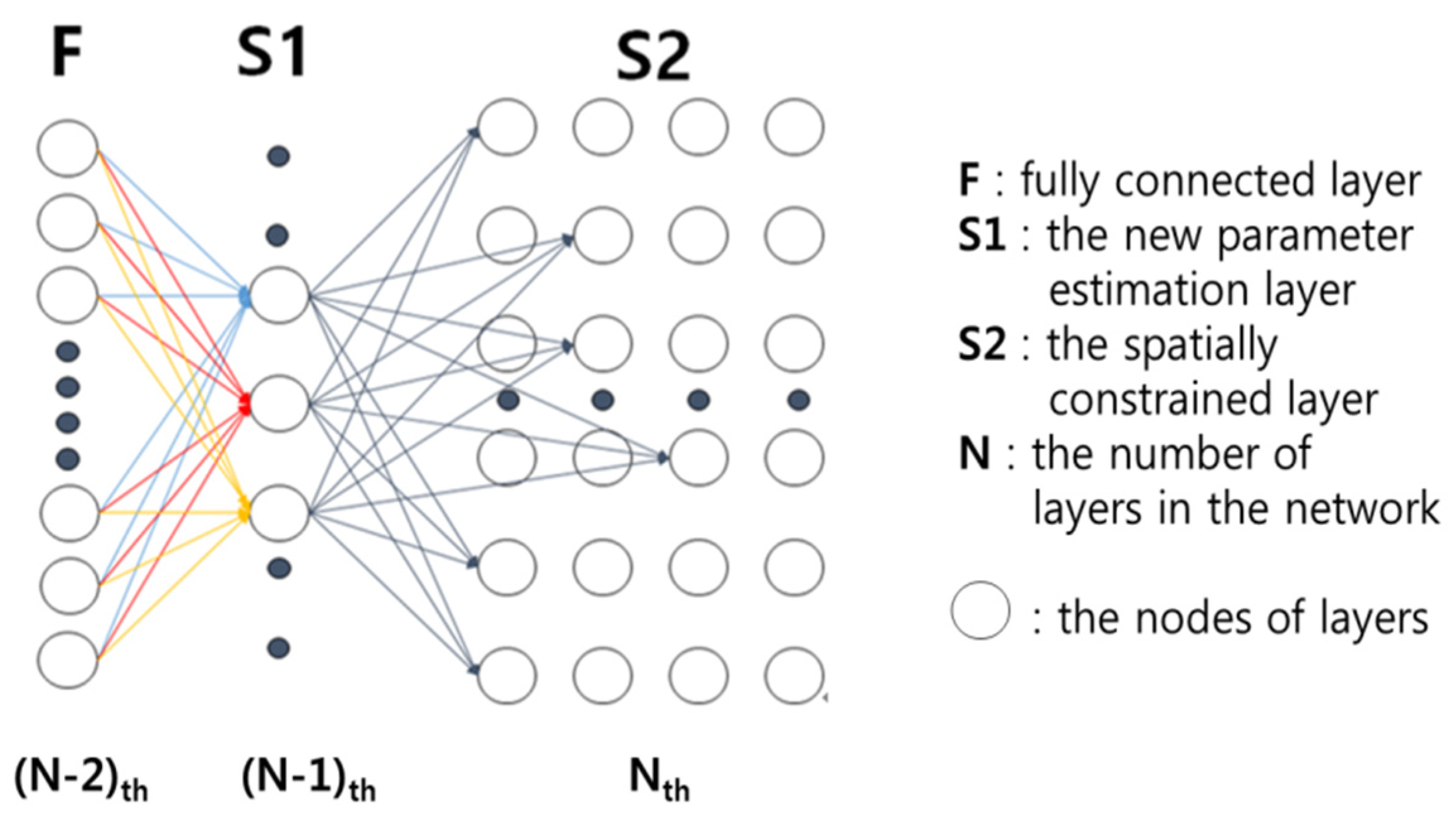
In [18], they proposed a spatially constrained convolutional neural network (SC-CNN) to perform nucleus detection. SC-CNN regresses the likelihood of a pixel being the center of a nucleus, where high probability values are spatially constrained to locate in the vicinity of the center of nuclei. For the classification of nuclei, they propose a novel neighboring ensemble predictor (NEP) coupled with CNN to more accurately predict the class label of the detected cell nuclei. Figure 1 shows the structure of the SC-CNN.
In reference [19], they propose a new deep architecture that uses support vector machines (SVMs) with class probability output networks (CPONs) to provide better generalization power for pattern classification problems. As a result, deep features are extracted without additional feature engineering steps, using multiple layers of the SVM classifiers with CPONs. The proposed structure closely approaches the ideal Bayes classifier as the number of layers increases.
In reference [20], a novel approach is proposed for training deep convolutional neural networks (DCNNs) that allows us to trade-off complexity and accuracy to learn lightweight models suitable for robotic platforms such as AgBot II (which performs automated weed management). Their approach consists of three stages. The first is to adapt a pre-trained model to the task at hand. This provides state-of-the-art performance but at the cost of high computational complexity, resulting in a low frame rate of just 0.12 frames per second (fps). The second is to use the adapted model and employ model compression techniques to learn a lightweight DCNN that is less accurate but has two orders of magnitude fewer parameters. The third is to combine K lightweight models as a mixture model to further enhance the performance of the lightweight models.
In reference [21], two implementations of the multiple-expert color feature extreme learning machine (MEC-ELM) are presented. The MEC-ELM is a cascading algorithm that has been implemented alongside a summed area table (SAT) for fast feature extraction and object classification, for a fully functioning object detection algorithm. The MEC-ELM is an implementation of the color feature extreme learning machine (CF-ELM), which is an extreme learning machine (ELM) with a partially connected hidden layer, taking three color bands as inputs.
In reference [22], research developments conducted within the last 15 years on machine learning based techniques for accurate crop yield prediction and nitrogen status estimation are discussed. They conclude that the rapid advances in sensing technologies and ML techniques will provide cost-effective and comprehensive solutions for better crop and environment state estimation and decision making.
In [23], an integrated self-diagnosis system (ISS) is proposed for an autonomous vehicle based on an IoT gateway and deep learning that collects information from the sensors of an autonomous vehicle, diagnoses itself and the influence between its parts by using deep learning, and informs the driver of the result. ISS reduces loss of life and overall cost by transferring the self-diagnosis information and by managing the time to replace the car parts of an autonomously driven vehicle safely.
3. A Total Crop-Diagnosis Platform (TCP) Based on Deep Learning Models in a Natural Nutrient Environment
3.1. Overview
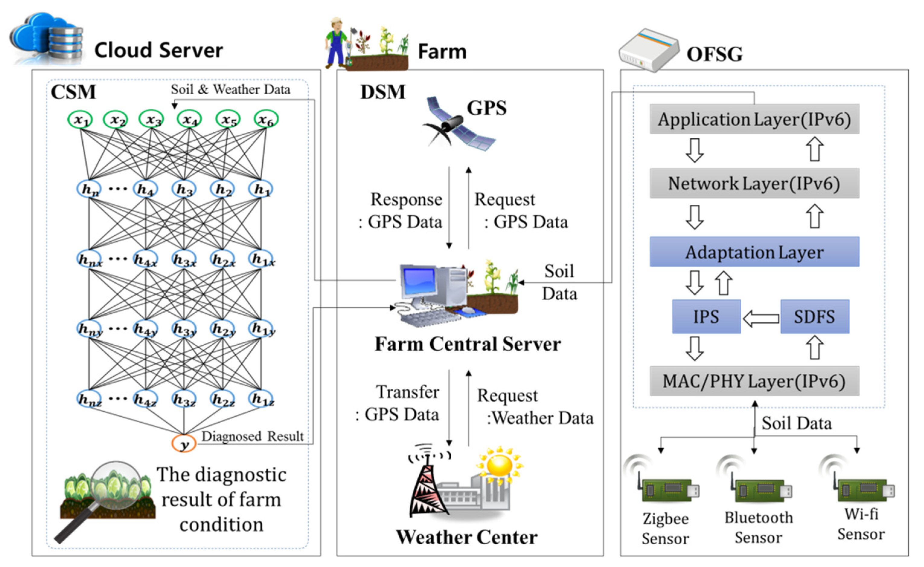
The proposed TCP collects the weather information based on a farm’s location information, diagnoses the collected weather information and the crop soil sensor data with a deep learning technique, and informs a farm manager of the diagnosed result. Figure 2 shows the structure of TCP. The proposed TCP is composed of 1 gateway and 2 modules as follows. First, the optimized farm sensor gateway (OFSG) collects soil data by internetworking sensor nodes which use Zigbee, Wi-Fi and Bluetooth protocol, reduces the number of sensor data fragmentation times through the compression of a fragment header and transfers the collected soil data to the DSM. Second, the data storage module (DSM) receives the collected soil data from the OFSG and stores it and the weather data from the weather center in a farm central server. The DSM transfers the stored data to the CSM. Third, the crop self-diagnosis module (CSM) works in the cloud server and diagnoses by deep learning whether or not the status of a farm is in good condition for growing crops with the soil data and weather data transferred from the DSM. The CSM transfers the diagnosed result to the farm central server of the DSM.
3.2. A Design of an Optimized Farm Sensor Gateway (OFSG) Based on Wireless Sensor Network
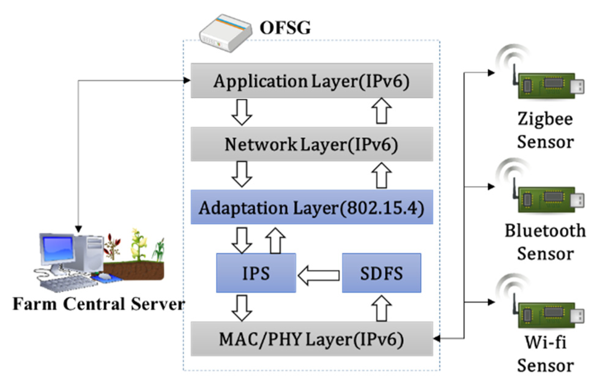
The proposed OFSG consists of an application layer, a network layer, an adaptation layer, and a media access control/physical (MAC/PHY) layer as shown in Figure 3. Because the application layer, the network layer, and the MAC/PHY layer among these are based on IPv6 protocol, this paper covers just the adaptation layer. A farm central server requests data collection to the application layer. The application layer delivers the request to a network layer and the network layer delivers the request to an adaptation layer by turns. Finally, the adaptation layer delivers the request to a MAC/PHY layer. The MAC/PHY layer collects the sensor data from the sensors of diverse environments and delivers the collected data to the farm central server through the adaptation layer by using compression and fragmentation.
Here, the adaptation layer is composed of two sub-modules as follows. First, an interconnection protocol sub-module (IPS) collects data by interconnecting sensor nodes which uses Zigbee, Wi-Fi and Bluetooth in diverse communication environments. Second, because the maximum data size that sensor nodes can transmit is 127 bytes, they have to transfer the fragments by data fragmentation. A sensor data fragment sub-module (SDFS) reduces the number of sensor data fragmentation times through the compression of this fragment header. The fragment’s payload size is increased to a maximum of 101 bytes.
3.2.1. A Design of an Interconnection Protocol Sub-Module (IPS)
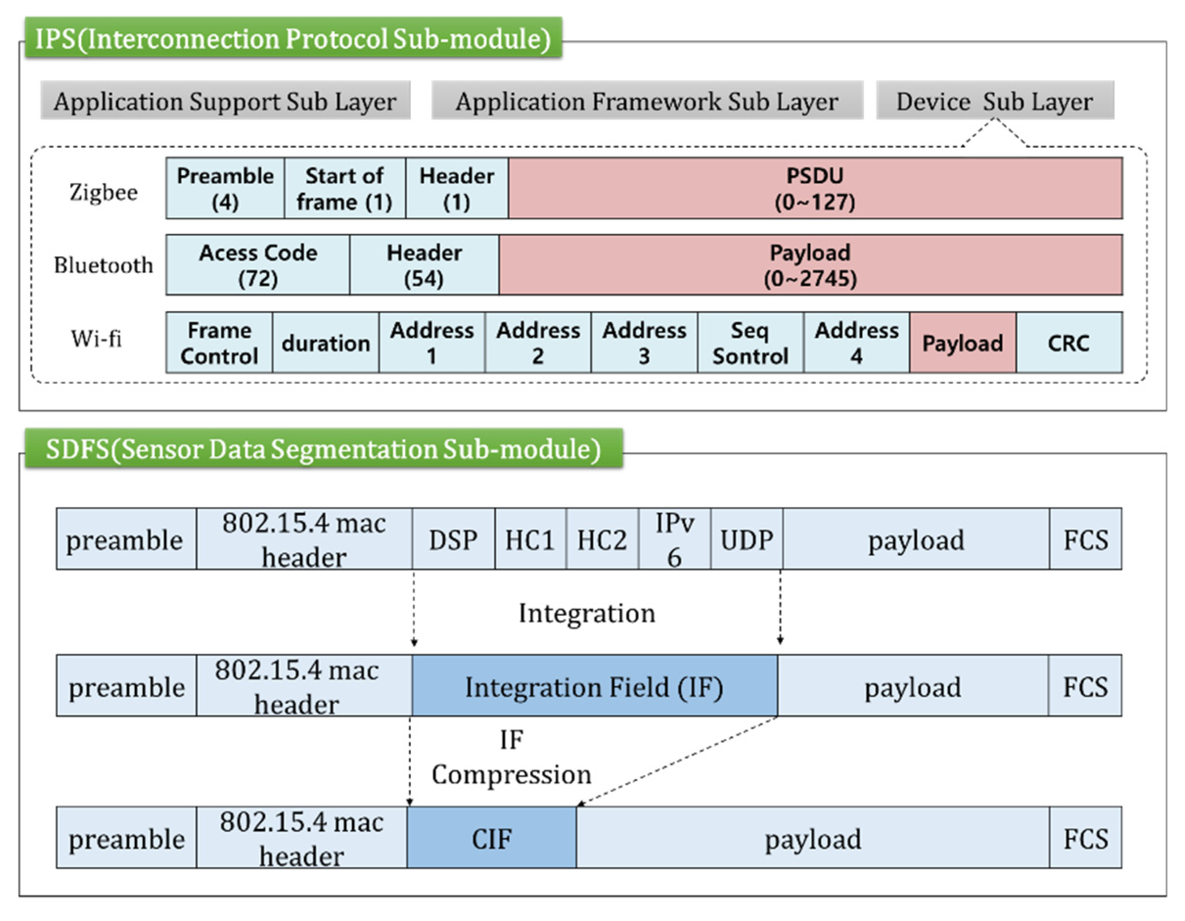
The IPS consists of three sub-layers as shown in Figure 4. The first application support sub-layer acts as an interface when a farm central server delivers a request message to sensor nodes, and the sensor nodes delivers the response data to the farm central server. The application framework sub-layer manages the applications about Zigbee, Wi-Fi, and Bluetooth equipped on the sensor nodes. The device sub-layer analyzes the Zigbee, Bluetooth and Wi-Fi protocol to internetwork sensor nodes. For example, the device sub-layer receives a frame from a Wi-Fi device as shown in Figure 4, extracts a payload from it and stores the payload in a cache. Zigbee and Bluetooth extract physical service data unit (PSDU) (or payload) in the same way and write the PSDU and identification information in a cache.
The payload stored in the cache is fragmented in the SDFS and the fragments are delivered to the farm central server through the application framework sub-layer and the application support sub-layer.
3.2.2. A Design of a Sensor Data Fragmentation Sub-Module (SDFS)
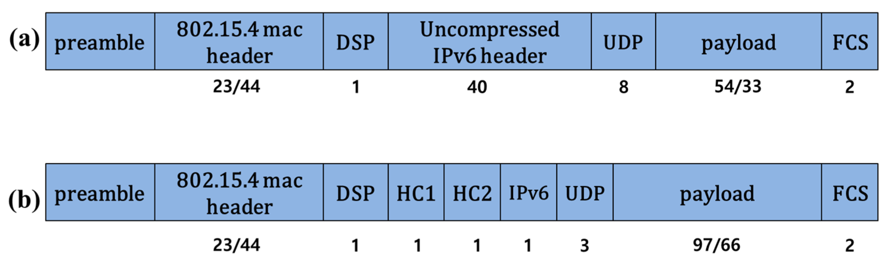
Because the size of the sensor data to be transferred one at a time is limited in a wireless sensor node, the sensor node generates messages of 127 bytes as shown in Figure 5. Figure 5a represents the data format used for wireless communication and Figure 5b represents the changed data format of Figure 5a when the basic compressed method of IPv6 over Low power Wireless Personal Area Network (6LoWPAN) was applied to Figure 5a. The SDFS works in the following steps.
First, the SDFS fragments them to transfer the messages received from the sensor nodes to the farm central server. Figure 5a shows the received message format.
Second, the SFDS compresses the headers of fragments by using the compression technique provided by 6LoWPAN. The uncompressed header IPv6 header (40 bytes) and User Datagram Protocol (UDP) (8 bytes) of Figure 5a are compressed to header compression 1(HC1) (1 byte), header compression 2 (HC2) (1 byte), IPv6 (1 byte), and UDP (3 bytes) of Figure 5b. Figure 5b shows the compressed message format.
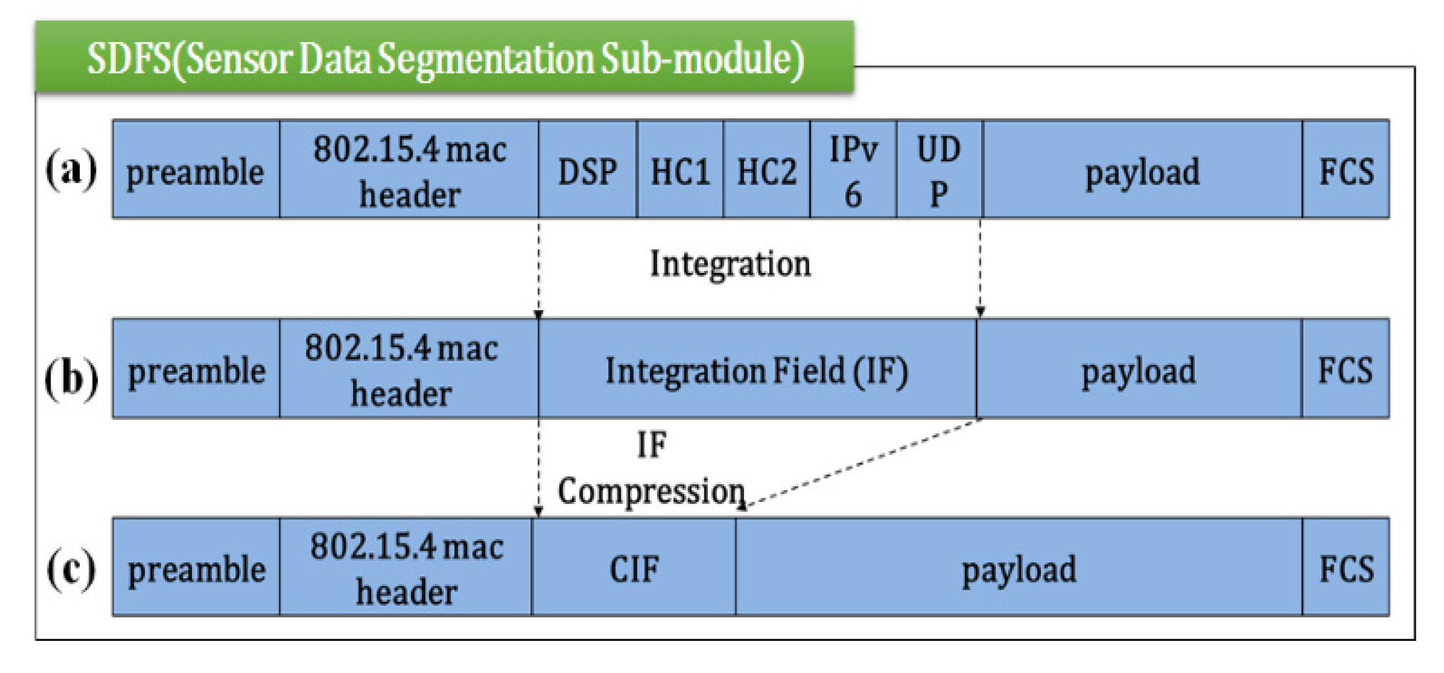
Third, in Figure 6b,c, the SDFS expands the maximum transmission size by integrating the fields of the compressed headers and compressing them again.
Therefore, the SDFS reduces the transmission cost of sensor data and makes the transmitted payload size larger at the same time.
The SDFS improves the fragmentation process to solve the problem that the data size transmitted at one time is limited in the wireless sensor network. The size of each fragment by fragmentation is 127 bytes, and a header and payload are included in the fragment. However, fragmentation happens frequently because the transmitted payload size is reduced as the header size gets larger.
To solve this problem, the SDFS minimizes the header size and maximizes the payload size. All the fields except the hop limit field are compressed in the existing 6LoWPAN and only the header—except version, source/destination address, payload length, traffic class, flow label, next header fields—is compressed in the SDFS. The compression shows that the payload size is a maximum of 97 bytes. The DSP, HC1, HC2, IPv6, and UDP field in the compressed header in the wireless sensor network is 1~3 bytes long. Because the 5 fields cannot be compressed or fragmented further, the size of the payload transmitted at one time is limited to 97 bytes. Figure 6a,b shows that the DSP, HC1, HC2, IPv6 and UDP fields of the header are integrated into one integrated field (IF).
In Figure 6c, if the IF is compressed, the header becomes smaller and the payload becomes bigger. The payload becomes a maximum of 101 bytes long. Here, if the payload size becomes bigger, the number of data fragmentation times is smaller.
3.3. A Design of a Data Storage Module (DSM)
The DSM collects the weather data from the weather forecast service on the basis of the location of a farm and the soil data from the OFSG in real time and stores them in the inner buffer. Figure 7 shows the structure of the DSM. It works as follows.
First, the DSM collects its own location information through GPS. Second, the DSM collects the weather data, such as the temperature, humidity, sunshine amount, wind amount, wind speed, etc., by transferring the location of a farm central server to the weather forecast service and stores it in the internal data buffer. Third, the DSM collects the data of multiple elements in real time from the sensor in the soil where crops are planted and stores it in the buffer. Fourth, the DSM transfers the weather and soil information stored in the buffer to a cloud server.
3.4. A Design of a Crop Self-Diagnosis Module (CSM) Based on Deep Learning
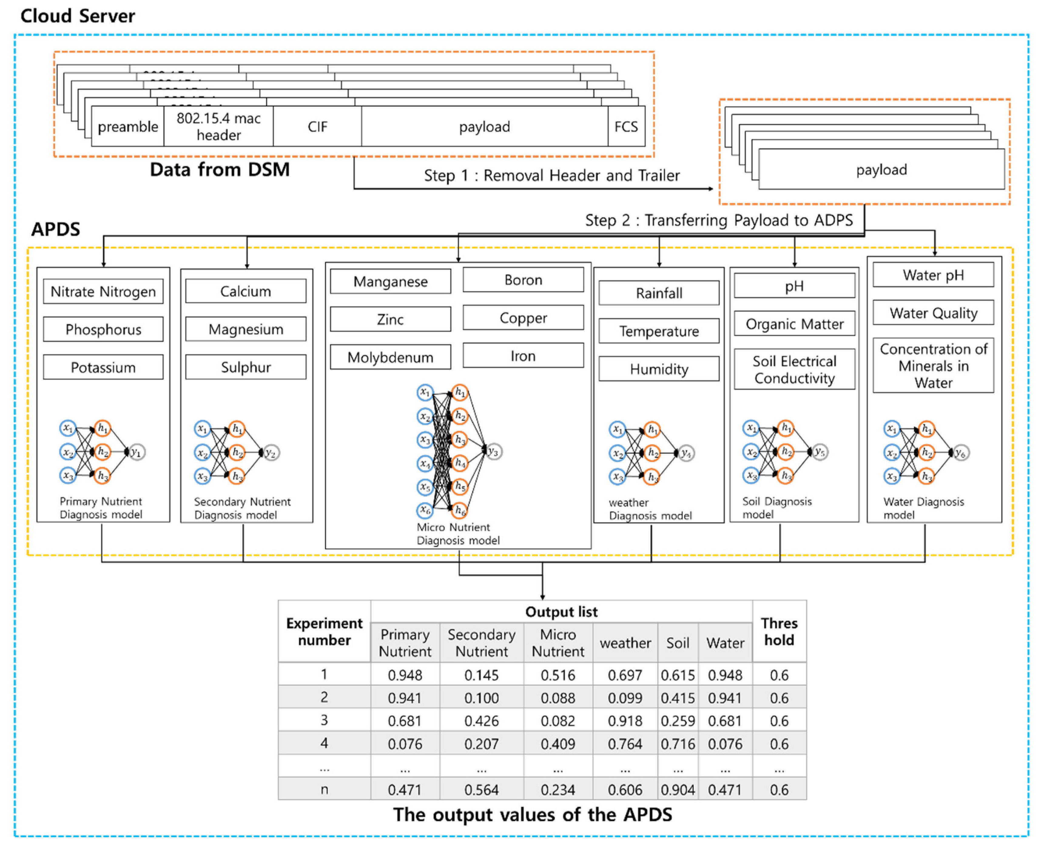
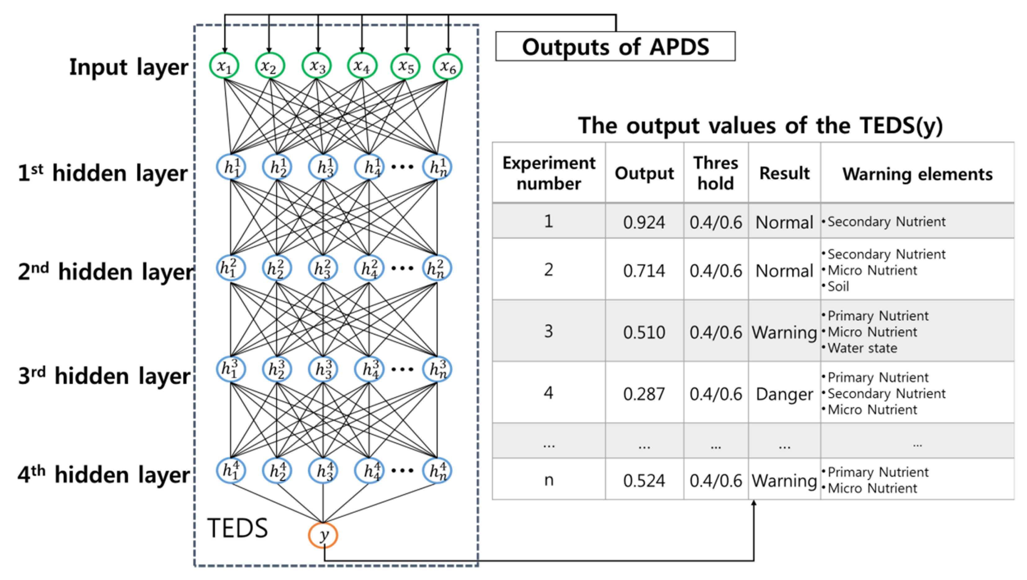
The CSM works in the cloud server. The CSM diagnoses whether the state of a farm is in a good condition for growing crops according to the current weather and soil information and informs a farmer of the diagnosed result. The CSM is composed of two sub-modules. First, the agricultural partial diagnosis sub-module (APDS) diagnoses each part of a farm environment by using sensor data from sensors. Second, the total environment diagnosis sub-module (TEDS) diagnoses the total status of a farm environment based on each partial diagnosis which was analyzed by the APDS.
The APDS classifies the sensor data into primary nutrient, secondary nutrient, micro nutrient, weather, soil, and water. The classified data is used as an input data for six neural network models, and an output value between 0 and 1 is generated from six neural network models as shown in Figure 8. The output value of the APDS represents the status of each partial diagnosis and is used as an input of the TEDS. For example, Figure 8 shows the output value of the APDS. The output value becomes the input value of the TEDS. If the output of the TEDS is decided, the TCP informs a farmer of only the “danger” or the “warning” necessary to check among the results of the TEDS and the APDS.
3.4.1. A Design of the APDS
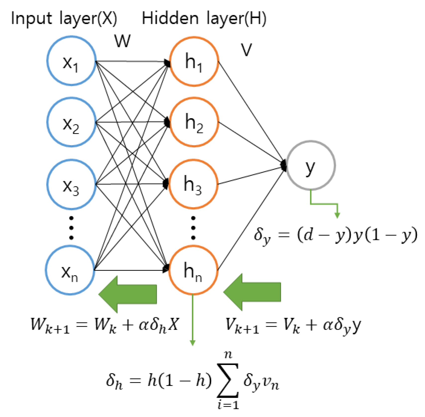
The APDS has the multi-layered neural network models which use back-propagation learning. In Figure 8, the APDS consists of the six neural network models which diagnose the parts affecting farming. For example, each part means the primary and secondary nutrient of soil, micro nutrient, weather and soil condition separately. Sensor data is used as an input of a neural network model suitable for each diagnosis. The APDS uses the sensor data (see Figure 6c) transferred from the DSM as an input. In order for the APDS to be able to use the sensor data normally, the cloud server extracts payloads by removing the header and trailer from the sensor data (see step 1 of Figure 8). Then, the cloud server transfers the extracted payloads to the APDS (see step 2 of Figure 8). Because the OFSG transforms different formats into one format, the APDS processes only the payloads with one format. Also, because the payloads have the same size, the APDS has no problem in processing them. If the number of sensors is n, the input of the APDS is represented as the following Formula (1).
Because the output results of the six parts are not classified linearly, each neural network model has only one hidden layer. The number of hidden layer nodes is the same as that of input layer nodes. The hidden layer is represented as the following Formula (2).
The output of the APDS is represented as one node, y which means the status of each part. The weight W between an input layer and a hidden layer is represented as the following Formula (3).
The weight V between a hidden layer and an output layer is represented as the following Formula (4).
Because the number of hidden layers is the same as that of input layers, the number of weights W is n × n. Figure 9 shows one example of the six neural network models in the APDS.
The output y of each neural network models is between 0 and 1, and the items entered in the current neural network models are used as the value to judge whether farming is in a good condition. For example, in Figure 8, the first case shows that the analysis result of the primary nutrient is 0.948 and it is normal numeric is as much as 94.8%. The results of the six neural network models in the APDS are entered in the TEDS.
The APDS is learned by using the back-propagation. Algorithm 1 shows the learning method of a neural network models in the APDS.
Algorithm 1 works as follows.
- First, the set of sensor data Xi and the result of Xi, di are entered into a neural network model;
- Second, the APDS initializes input layer size n, weight w, learning rate α and limitation value of error Emax;
- Third, the APDS computes the value of the hidden layer nodes by using Formulas (5) and (6);
- Fourth, the APDS computes the values of the output layer node by using Formulas (7) and (8):
- Fifth, the APDS computes the error E and the error signal by using the value of the output layer node and current trained result value, di. Formulas (9)–(11) are used to compute E and , separately:
- Sixth, the APDS modifies the weight V and W of a neural network model by using Formulas (12) and (13). The V represents the weight between the output layer and the hidden layer and W the weight between the input layer and the hidden layer:
If the process from the 3rd to the 6th is repeated as many times as the number of trained samples, the current error E and Emax are compared. If the E is less than Emax, the APDS learning is closed. If the Emax is less, the APDS converts E to 0 again and the APDS learning proceeds repeatedly.
| Algorithm 1 APDS learning method |
| Input = Training samples {X1, d1}, …, {XN, dN}; (Xi is set of sensor data, di is result of Xi) Run: Initialize sample weight w; n is the number of input layers and hidden layer nodes; Set learning rate α and Emax; while (E < Emax) E = 0; for (int j = 1; j <= N; j++) Classify sensors of Xj; Compute output of hidden layer ; Compute output; Compute output error Compute error signal of output layer Compute error signal of hidden layer Update weights j++; end for; end while; |
3.4.2. A Design of the TEDS
The TEDS performs deep learning based on the multi-layered deep belief network model (DBN). If the number of input layer nodes in the DBN is the same as that of the output layer nodes, unsupervised learning is possible. However, because the number of input layer nodes in the TEDS is different from that of the output layer nodes, unsupervised learning based on the restricted Boltzmann machine (RBM) is done from the input layer to the last hidden layer and supervised learning based on back-propagation is done between the last hidden layer and the output layer. Figure 10 shows the example of the integrated model in the TEDS.
The six outputs of the APDS are used for the six inputs of the TEDS. This is represented in Formula (14).
y is the output of the TEDS and represents how suitable the current environmental state is for the growing crops. The size of y is between 0 and 1 and the threshold values of y are 0.4 and 0.6. If the output of y is equal to or greater than 0.6, it means that the current environmental state is in a good condition for farming. If the output of y is between 0.6 and 0.4, it means that the current environmental state should be checked. If the output of y is less than 0.4, the current environmental state is not in a good condition for farming. Figure 11 shows the structure of the TEDS. The number of hidden layers is set as 4. Because the number of input and output layer nodes is smaller, the correlation between parts is computed with the four hidden layers by the TEDS. The hidden layers of the TEDS are represented in the Formula (15).
where k means the number of hidden layer nodes and means the number of hidden layers. For example, the 1st hidden layer and the nodes of the 1st hidden layer are represented as } and the 2nd hidden layer and the nodes of the 2nd hidden layer are represented as }.
Algorithm 2 shows the learning procedure of the TEDS.
| Algorithm 2 TDS learning algorithm |
| Input = Training data {X1, d1}, …, {XN, dN}; (Xn is set of sensor data, dn is result of Xn) Run: Initialize sample weight w; n is the number of input layer nodes m[4] is set of the number of hidden layer nodes for (int k = 1; k <= m[0]; k++) Compute ; end for for (int n = 1; n <= 6; n++) Compute ; end for compute ; for (int k = 1; k <= m[0]; k++) Compute ; end for Compute ; ; ; for (int j = 2; j <= 4; j++) for (int k = 1; k <= m[j]; k++) calculator ; end for for (int k = 1; k <= m[j]; k++) Compute ; end for Compute ; for (int k = 1; k <= m[j]; k++) Compute ; end for Compute ; ; ; end for while (E > Emax) ; ; if (E > Emax) ; ; else brake; end if end while |
Each neuron’s computation method is similar to that of a perceptron. That is, the weight sum net of input layer values is applied to the Sigmoid function. For example, in Figure 11, the output value of is computed in the Formula (16).
where is a value of node when is used as an input. is a Sigmoid function used as an activation function in the artificial neural network, as shown in Formula (17).
where the represents the weight sum of input layer values. The is computed in Formula (18).
Because an RBM-based learning is unsupervised learning, it is proceeded by using the value that computed the value from to again. The TEDS continues learning by using the following phase from the input layer to the last layer. In the 1st phase, the TEDS computes the 1st hidden layer value, . In the 2nd phase, the TEDS computes by using the value and the input value. The is computed by using Formula (19).
In the 3rd phase, the TEDS computes the input layer value, and the based on the . In the 4th phase, the TEDS compares the input value with the and the with the . The is computed in the same method as Formula (19). In the 5th phase, the difference amount of the weight between the input layer and the first hidden layer is computed in Formula (20) about the complete pair <n, k>.
where is a learning rate determined by a developer in advance and the weight is modified by using Formula (21).
The learning from the first hidden layer to the last hidden layer is repeated by the first phase to about the 5th phase. The TEDS continues learning between the last hidden layer and the output layer in the following phases.
In the 1st phase, it computes the output layer result . Here, the is assumed as .
In the 2nd phase, it computes error E by using the difference between and the target value . The is computed by using Formula (22).
In the 3rd phase, the error signal is computed by using Formula (23).
In the 4th phase, the weight between the last hidden layer and the output layer is modified by using the error signal .
In the 5th phase, the 2nd~4th phases are repeated if the error E is equal to and greater than the Emax. If the E is less than the Emax, the learning is closed.
4. The Performance Analysis
4.1. An Analysis of the OFSG Performance
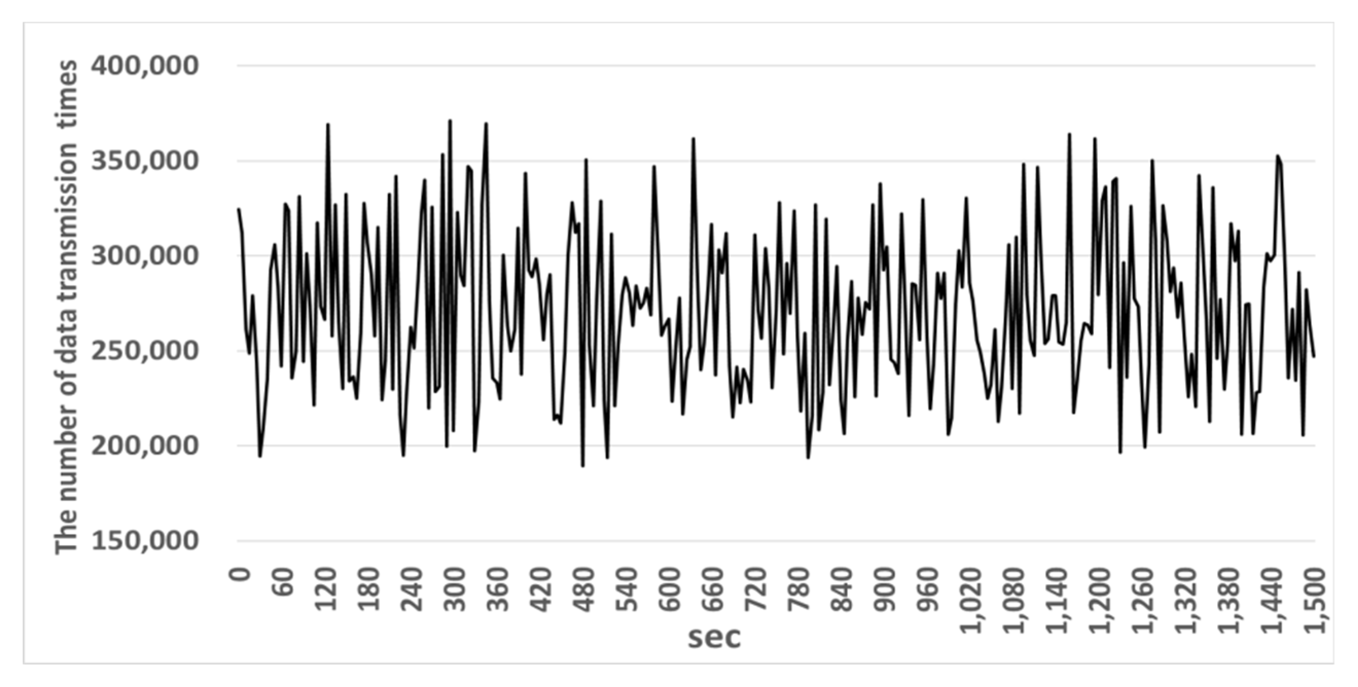
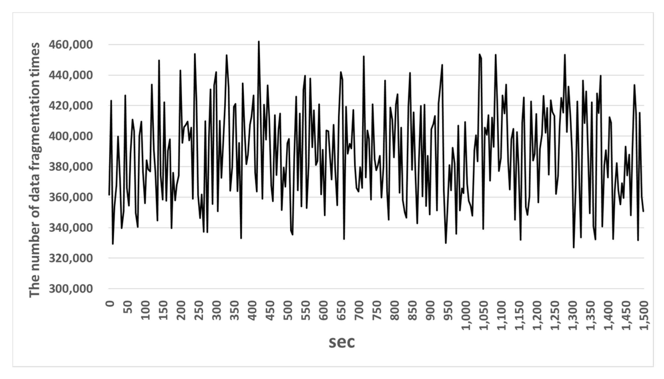
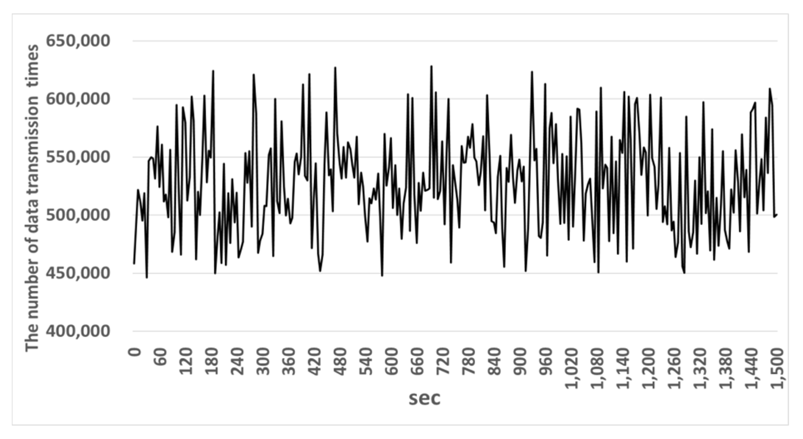
The OFSG extracts the payload from the sensor data and stores the extracted payload in a cache and transfers the stored payload cache to a farm central server after compression and fragmentation. The simulation environment of the OFSG is as follows.
First, the number of wireless sensor nodes is 20, the data size is 800 bytes, and the data generation cycle is 0.1 s.
Second, the experiment time is 1500 s, and data fragmentation and data transmission quantity are measured by the 5 s.
Third, the existing wireless sensor gateway not using fragmentation and compression and the OFSG using them are compared in terms of their data fragmentation and transmission quantity.
Fourth, when one message is fragmented into all fragments, it is called one data fragmentation. The number of data fragmentation times is the same as that of messages.
Figure 12 and Figure 13 show the number of data fragmentation times and data transmission quantity in the existing gateway. Figure 14 and Figure 15 show the number of data fragmentation times and data transmission quantity in the OFSG.
The experiment shows that in Figure 12 an existing gateway fragmented 189,325~371,283 messages and in Figure 13 transferred 153,398~247,036 messages of them. Therefore, the message transmission rate of the existing gateway was 66.53%. In Figure 14 the OSFG fragmented 446,110~628,115 messages and in Figure 15, transferred 326,954~461,935 messages of them. Therefore, the message transmission rate of the OSFG was 73.5% and was improved by about 7% compared with the existing gateway. Therefore, the reason why this experiment result was improved is because the OSFG used the compression and fragmentation technique applied to headers. If the headers are used, a bigger payload can be stored in a fragment. As the size of the field that can store a payload gets larger, the message is fragmented into a smaller number of fragments and is processed faster.
4.2. The Analysis of the CSM Performance
To analyze the performance of the CSM, the APDS and the TEDS should be simulated beforehand. If the number of the APDS’s hidden layers gets larger, this paper measures the number of repeated learning times and the accuracy of the APDS. If different activation functions are used, this paper measures the accuracy of a neural network model. In addition, this paper analyzes the learning speed and reliability of each neural network model by comparing the proposed TEDS neural network model, long short-term memory (LSTM) neural network model and convolutional neural network (CNN) neural network model. The Server PC using the GeForce GTX 1080 CPU and the Client PC transferring sensor data are used for the simulation environment.
4.2.1. The Analysis of the APDS Performance
To analyze the APDS performance, the initial weight, the initial learning rate, and the learning reduction rate of each algorithm that a developer should set at the initial learning stage are used as control variables. Table 1 shows the control variables to analyze the APDS performance.
Figure 16 shows the average repeated learning times and the average error rate according to the number of hidden layers of the six neural network models of the APDS.
In case there is no hidden layer, the APDS neural network models learn fastest when the number of average repeated learning times is 100, but they do not classify data when an error rate is 52.9%. In case there isone1 hidden layer, the APDS neural network models show that the number of average repeated learning times is 249 and the error rate is 3.1%. In case there are six hidden layers, the APDS neural network models show that the number of average repeated learning times is 898 and the error rate is 2.8%.
In case there are hidden layers in the APDS neural network models, the error rate is about 0.5%. However, because the average repeated learning times are increased in proportion to the number of hidden layers, the APDS neural network models have to use just one hidden layer.
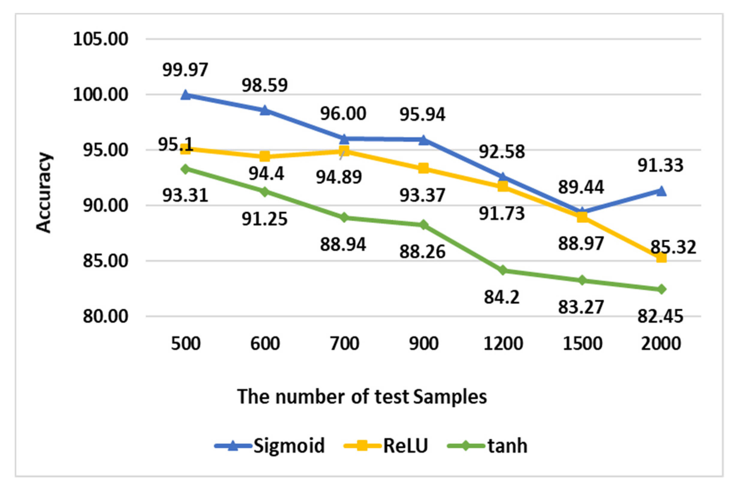
Figure 17 shows the accuracy according to test data when the APDS neural network models that used one hidden layer use the Sigmoid function and a tanh function as an activation function.
When a Sigmoid function was used as an activation function and the number of test samples was 500, the accuracy was measured as 99.97%. When the number of test samples was 700, the accuracy was measured as 96%. When the number of test samples was 1200, the accuracy was measured as 92.587%. Finally, when the number of test samples was 2000, the accuracy was measured as 91.337%.
When a rectified linear unit (ReLU) function was used as an activation function and the number of test samples was 500, the accuracy was measured as 95.1%. When the number of test samples was 700, the accuracy was measured as 94.89%. When the number of test samples was 1200, the accuracy was measured as 91.73%. Finally, when the number of test samples is 2000, the accuracy was measured as 85.32%.
When a tanh function was used as an activation function and the number of test samples was 500, the accuracy was measured as 93.31%. When the number of test samples was 700, the accuracy was measured as 88.94. When the number of test samples was 1200, the accuracy was measured as 84.2%. Finally, when the number of test samples was 2000, the accuracy was measured as 82.45%.
In summary, if a Sigmoid function is used as an activation function, the average accuracy is measured as 94.84%. If a ReLU function is used, the average accuracy is measured as 91.97%. If a tanh function is used, the average accuracy is measured as 87.38%. Therefore, the Sigmoid function is increased by about 3% and 7% in accuracy compared with ReLU and tanh, respectively.
4.2.2. The Analysis of the TEDS Performance
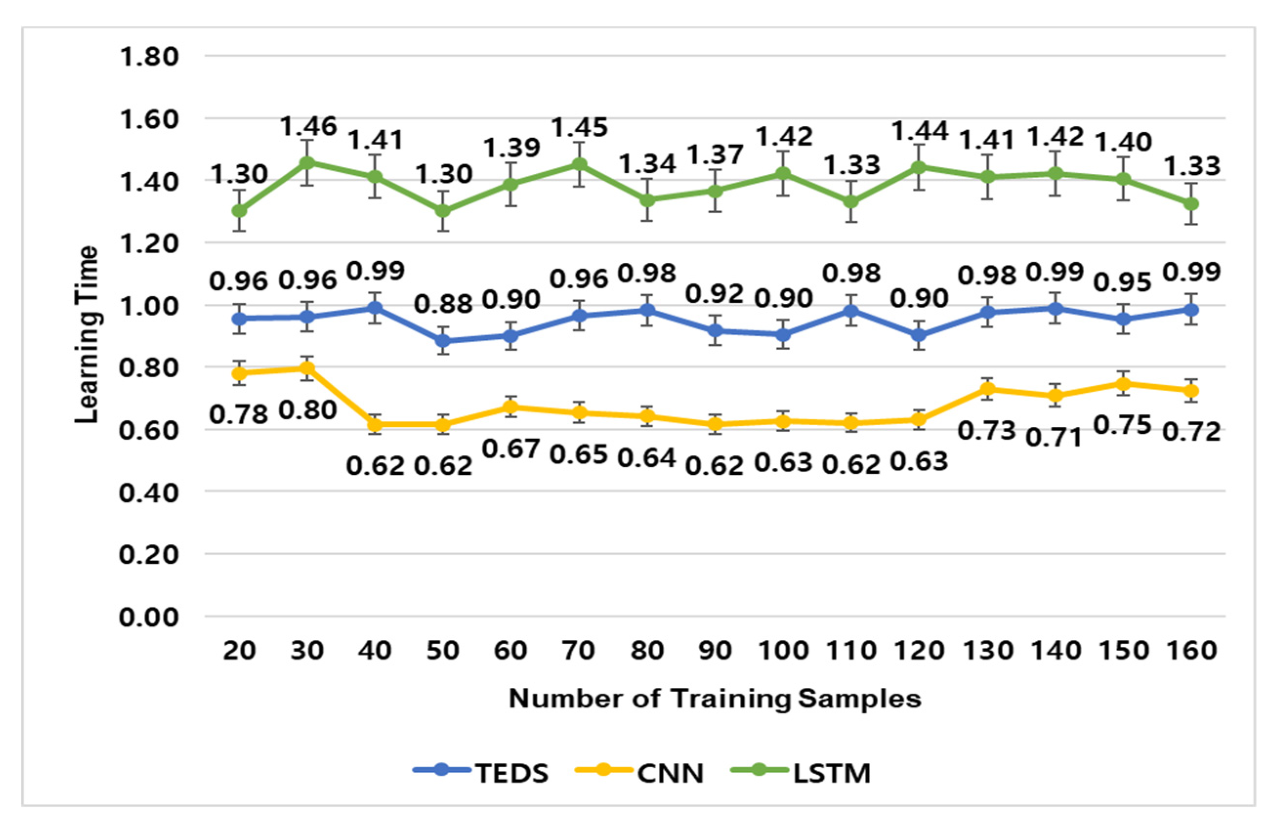
To analyze the TEDS performance, the number of hidden layers is set to 4. The number of nodes of each hidden layer is set to 15. The learning rate and weight are set at 0.1 separately. The experiment on the TEDS was performed twice and the result is as follows. The first experiment was to compare the learning time of neural network models according to training samples. Figure 18 shows the result.
In the TEDS in Figure 18, when the number of the training samples is 21, the learning time is 0.96. When the number of training samples is 80, the learning time is 0.98. When the number of training samples is 120, the learning time is 0.90. When the number of the training samples is 150, the learning time is 0.95. The average learning time of the TEDS is 0.95. In the CNN in Figure 18, when the number of the training samples is 21, the learning time is 0.78. When the number of the training samples is 80, the learning time is 0.65. When the number of the training samples is 120, the learning time is 0.63. When the number of the training samples is 150, the learning time is 0.75. The average learning time of the CNN is 0.68.
In the LSTM in Figure 18, when the number of the training samples is 21, the learning time is 1.30. When the number of the training samples is 80, the learning time is 1.34. When the number of the training samples is 120, the learning time is 1.44. When the number of the training samples is 150, the learning time is 1.4. The average learning time of the LSTM is 1.38.
Therefore, the learning time of the TEDS is faster than that of the LSTM by about 0.43 and slower than the CNN by about 0.27. However, the following second experiment shows that the TEDS is better than the CNN in farm diagnosis.
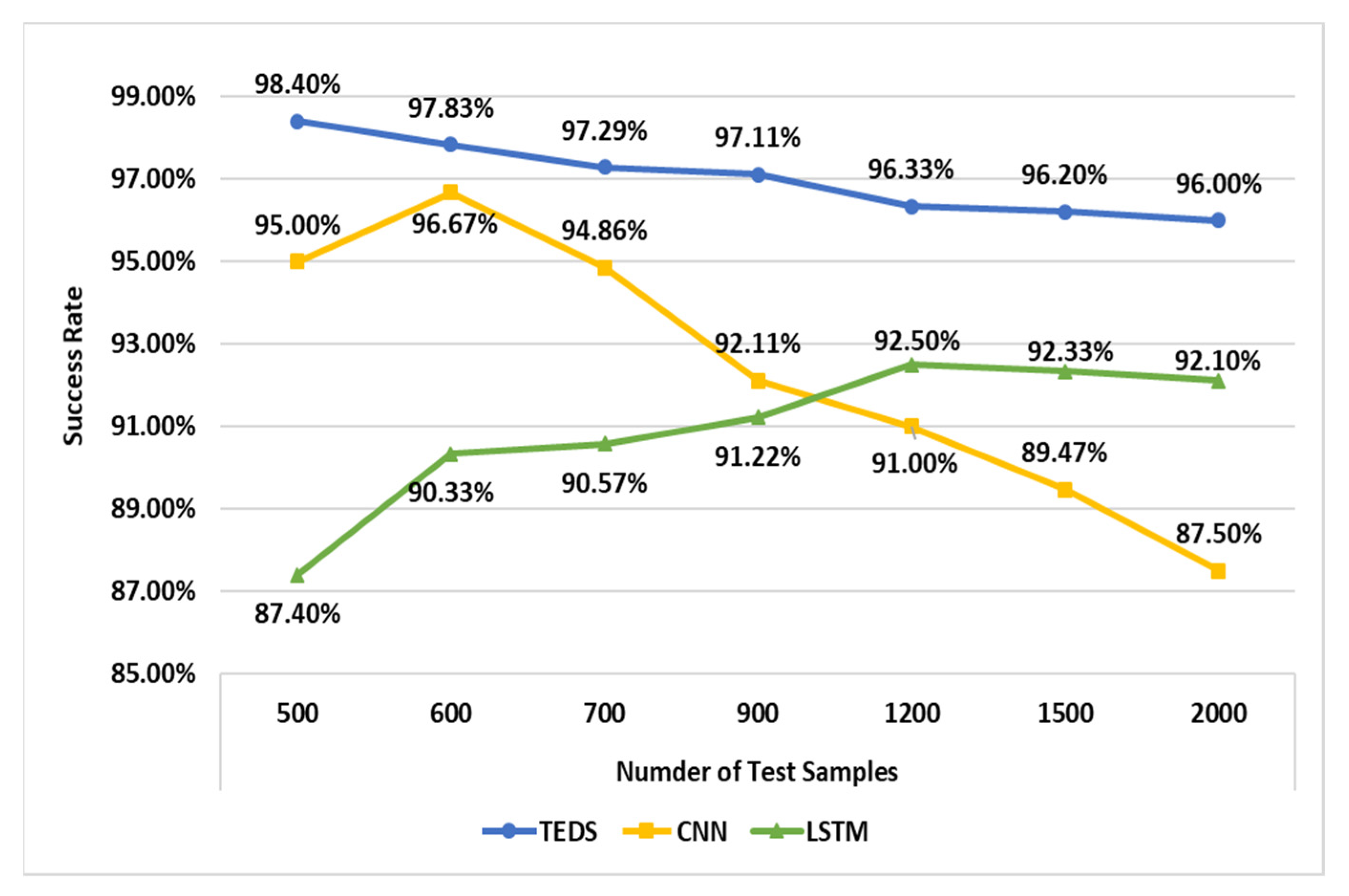
The second experiment was to compare the diagnosis success rate according to the test samples. The result is shown in Figure 19.
In the TEDS neural network models in Figure 19, when the number of the training samples is 500, the diagnosis success rate is measured as 98.40%. When the number of the training samples is 600, the diagnosis success rate is 97.83%. When the number of the training samples is 1200, the diagnosis success rate is 96.33%. When the number of the training samples is 2000, the diagnosis success rate is 96%.
In the CNN neural network models in Figure 19, when the number of the training samples is 500, the diagnosis success rate is measured as 95%. When the number of the training samples is 600, the diagnosis success rate is 96.67%. When the number of the training samples is 1200, the diagnosis success rate is 91%. When the number of the training samples is 2000, the diagnosis success rate is 87.5%.
In the LSTM neural network models of in Figure 19, when the number of the training samples is 500, the diagnosis success rate is measured as 87.40%. When the number of the training samples is 600, the diagnosis success rate is 90.33%. When the number of the training samples is 1200, the diagnosis success rate is 92.50%. When the number of the training samples is 2000, the diagnosis success rate is 92.10%.
In summary, the success rate of TEDS was higher than the CNN by an average of 5% and the LSTM by an average of 7%. For the CNN, when the number of samples is small, the difference between the TEDS and the CNN is about 2%. When the number of samples is 2000, the difference between the TEDS and the CNN is about 9%. For the LSTM, as the number of samples gets larger, the success rate is increased, but the success rate of the LSTM is much lower than that of the TEDS.
In summary, in the first experiment of learning time, the TEDS is slower than the CNN by 0.27 and faster than the LSTM by 0.43 s. In the second experiment of success rate, the TEDS is higher than the CNN by an average of 5% and the LSTM by an average of 7%. The TEDS is slower than the CNN in learning speed, but as data gets increased, the success rate of the TEDS gets higher. Therefore, the TEDS is the best neural network model when the state of a farm is judged.
5. Conclusions
Because an existing smart farm has to diagnose only a specific area of a farm or prepare agricultural robots by function according to the environment of farms and the kinds of crops, they are expensive to use and to manage.
To solve these problems, this paper proposes a total crop-diagnosis platform (TCP) based on deep learning models in natural nutrient environment which collects the weather information based on a farm’s location information, diagnoses the collected weather information and the crop soil sensor data with a deep learning technique, and notifies a farm manager of the diagnosed result.
The TCP based on a cloud server does not depend on the environment of farms and the kinds of crops. Because the TCP does not need to buy and manage various agricultural robots, contrary to an existing farm, this cuts costs significantly. If the environment of farms and the kinds of crops are changed, the TCP has only to customize its software. In addition, the TCP based on deep learning interconnects the communication protocols of various sensors, solves the maximum data size that sensor can transfer, predicts in advance crop disease occurrence in the external environment, and provides important information to the farmers for managing their crops.
The proposed TCP has some expected effects, as follows.
First, the OFSG interconnects the various communication protocols of sensors and solves the limitation of data size that sensors can transfer. Second, because the OFSG uses the compression and fragmentation applied to the headers, the number of the fragmentation times gets smaller and the processing speed gets higher. Third, because the APDS uses a Sigmoid function as an activation function in analysis process, it is better than a tanh function by about 7% in accuracy. Fourth, the TEDS is faster than the LSTM by 0.43 in learning time and higher than the LSTM by about 7% in success rate. As the data size gets bigger, the success rate of the TEDS gets more stable.
However, the TCP also has the following uncertainty and limitations. First, it processed the experiment by using the past weather data which our weather center provides and the past soil data which our neighboring farms provides. Second, because a deep learning model designer has much difficulty in establishing a proper threshold value by analyzing past weather and soil data, it takes much time to find a proper threshold value during the initial design process.
In the future, if researchers including us can obtain and process experiments with real time weather and soil sensor data, more accurate and better results can be obtained in the experiments. In addition, researches will have to search for how to reduce the time to find a proper threshold value.
Author Contributions
B.L. proposed the idea. Y.J., S.S. and S.L. made the paper based on the idea and carried out the experiments in Korean Language. B.L. guided the research and translated the paper into English. All authors read and approved the final manuscript.
Funding
This work was supported by the Regional New Project Leader Training Project through the Ministry of Education and National Research Foundation of Korea (NRF-2016H1D5A1909417).
Conflicts of Interest
The authors declare no conflicts of interest.
Abbreviations
| IoT | Internet of Things |
| AI | Artificial intelligence |
| ICT | Information and communication technology |
| TCP | Total crop-diagnosis platform |
| OFSG | Optimized farm sensor gateway |
| DSM | Data storage module |
| CSM | Crop self-diagnosis module |
| CNN | Convolutional neural metwork |
| LSTM | Long short-term memory models |
| IPS | Interconnection protocol sub-module |
| SDFS | Sensor data fragment sub-module |
| APDS | Agricultural partial diagnosis sub-module |
| TEDS | Total environment diagnosis sub-module |
| Agbot | Agricultural robot |
References
- Beecham Research Ltd. Towords Smart Farming Agriculture Embracing the IoT Vision; Beecham Research Ltd.: Boston, MA, USA, 2014. [Google Scholar]
- Real World Deep Learning: Neural Networks for Smart Crops. Available online: https://www.kdnuggets.com/2017/11/real-world-deep-learning-neural-networks-smart-crops.html (accessed on 10 September 2018).
- Technology Quarterly the Future of Agriculture. Available online: https://www.economist.com/technology-quarterly/2016-06-09/factory-fresh (accessed on 12 September 2018).
- O’Grady, M.J.; O’Hare, G.M. Modelling the smart farm. Inf. Process. Agric. 2017, 4, 179–187. [Google Scholar] [CrossRef]
- Huang, Y.; Chen, Z.; Yu, T.; Huang, X.; Gu, X. Agricultural remote sensing big data: Management and applications. J. Integr. Agric. 2018, 17, 1915–1931. [Google Scholar] [CrossRef]
- Ravazzani, G.; Corbari, C.; Ceppi, A.; Feki, M.; Mancini, M.; Ferrari, F.; Gianfreda, R.; Colombo, R.; Ginocchi, M.; Meucci, S.; et al. From (cyber)space to ground: New technologies for smart farming. Hydrol. Res. 2016, 48, 656–672. [Google Scholar] [CrossRef]
- Margaret Rouse. Available online: https://internetofthingsagenda.techtarget.com/definition/ZigBee (accessed on 20 September 2018).
- Abane, A.; Daoui, M.; Bouzefrane, S.; Muhlethaler, P. NDN-over-ZigBee: A ZigBee support for Named Data Networking. Future Gener. Comput. Syst. 2017. [Google Scholar] [CrossRef]
- Santos, B.P.; Goussevskaia, O.; Vieira, L.F.; Vieira, M.A.; Loureiro, A.A. Mobile Matrix: Routing under mobility in IoT, IoMT, and Social IoT. Ad Hoc Netw. 2018, 78, 84–98. [Google Scholar] [CrossRef]
- Kamilaris, A.; Prenafeta-Boldú, F.X. Deep learning in agriculture: A survey. Comput. Electron. Agric. 2018, 147, 70–90. [Google Scholar] [CrossRef]
- Saeed, Q.A.; Asifullah, K.; Aneela, Z.; Anila, U. Wind power prediction using deep neural network based meta regression and transfer learning. Appl. Soft Comput. 2017, 58, 742–755. [Google Scholar]
- Ferentinos, K.P. Deep learning models for plant disease detection and diagnosis. Comput. Electron. Agric. 2018, 145, 311–318. [Google Scholar] [CrossRef]
- Lv, Y.; Duan, Y.; Kang, W.; Li, Z.; Wang, F. Traffic Flow Prediction with Big Data: A Deep Learning Approach. IEEE Trans. Intell. Transp. Syst. 2015, 16, 865–873. [Google Scholar] [CrossRef]
- Leng, J.; Jiang, P. A deep learning approach for relationship extraction from interaction context in social manufacturing paradigm. Knowl.-Based Syst. 2016, 100, 188–199. [Google Scholar] [CrossRef]
- Kahou, S.E.; Bouthillier, X.; Lamblin, P.; Gulcehre, C.; Michalski, V.; Konda, K.; Jean, S.; Froumenty, P.; Dauphin, Y.; Boulanger-Lewandowski, N.; et al. EmoNets: Multimodal deep learning approaches for emotion recognition in video. J. Multimodal User Interfaces 2015, 10, 99–111. [Google Scholar] [CrossRef] [Green Version]
- Jirayucharoensak, S.; Pan-Ngum, S.; Israsena, P. EEG-based emotion recognition using deep learning network with principal component based covariate shift adaptation. Sci. World J. 2014. [Google Scholar] [CrossRef] [PubMed]
- Yang, Y.; Wu, Z.; Xu, Q.; Yan, F. Deep Learning Technique-Based Steering of Autonomous Car. Int. J. Comput. Intell. Appl. 2018, 17, 1850006. [Google Scholar] [CrossRef]
- Sirinukunwattana, K.; Raza, S.E.A.; Tsang, Y.; Snead, D.R.J.; Cree, I.A.; Rajpoot, N.M. Locality Sensitive Deep Learning for Detection and Classification of Nuclei in Routine Colon Cancer Histology Images. IEEE Trans. Med. Imaging 2016, 35, 1196–1206. [Google Scholar] [CrossRef] [PubMed]
- Sangwook, K.; Zhibin, Y.; Man, K.R.; Minho, L. Deep learning of support vector machines with class probability output networks. Neural Netw. 2015, 64, 19–28. [Google Scholar]
- McCool, C.; Perez, T.; Upcroft, B. Mixtures of Lightweight Deep Convolutional Neural Networks: Applied to Agricultural Robotics. IEEE Robot. Autom. Lett. 2017, 2, 1344–1351. [Google Scholar] [CrossRef]
- Sadgrove, E.J.; Falzon, G.; Miron, D.; Lamb, D.W. Real-time object detection in agricultural/remote environments using the multiple-expert colour feature extreme learning machine (MEC-ELM). Comput. Ind. 2018, 98, 183–191. [Google Scholar] [CrossRef]
- Chlingaryan, A.; Sukkarieh, S.; Whelan, B. Machine learning approaches for crop yield prediction and nitrogen status estimation in precision agriculture: A review. Comput. Electron. Agric. 2018, 151, 61–69. [Google Scholar] [CrossRef]
- Jeong, Y.; Son, S.; Jeong, E.; Lee, B. An Integrated Self-Diagnosis System for an Autonomous Vehicle Based on an IoT Gateway and Deep Learning. Appl. Sci. 2018, 8, 1164. [Google Scholar] [CrossRef]
Figure 1.
Structure of the spatially constrained convolutional neural network (SC-CNN).

Figure 2.
The structure of the total crop-diagnosis platform (TCP). CSM: the crop self-diagnosis module; DSM: the data storage module; OFSG: the optimized farm sensor gateway; IPS: an interconnection protocol sub-module; SDFS: a sensor data fragment sub-module.
Figure 2.
The structure of the total crop-diagnosis platform (TCP). CSM: the crop self-diagnosis module; DSM: the data storage module; OFSG: the optimized farm sensor gateway; IPS: an interconnection protocol sub-module; SDFS: a sensor data fragment sub-module.

Figure 3.
Structure of the optimized farm sensor gateway (OFSG).

Figure 4.
Structure of the interconnection protocol sub-module (IPS). PSDU: physical service data unit; CRC: cyclic redundancy check; DSP: dispatch code; HC: header compression; UDP: user datagram protocol; CIF: compressed integration field; FCS: frame check sequence.
Figure 4.
Structure of the interconnection protocol sub-module (IPS). PSDU: physical service data unit; CRC: cyclic redundancy check; DSP: dispatch code; HC: header compression; UDP: user datagram protocol; CIF: compressed integration field; FCS: frame check sequence.

Figure 5.
The compression technique of IPv6 over Low power Wireless Personal Area Network (6LoWPAN).
Figure 5.
The compression technique of IPv6 over Low power Wireless Personal Area Network (6LoWPAN).

Figure 6.
The fragment using a compressed integration field (CIF).

Figure 7.
The structure of the data storage module (DSM).

Figure 8.
The structure of the agricultural partial diagnosis sub-module (APDS).

Figure 9.
The one example of the six neural network models in the APDS.

Figure 10.
The example of the integrated model in the total environment diagnosis sub-module (TEDS).
Figure 10.
The example of the integrated model in the total environment diagnosis sub-module (TEDS).

Figure 11.
The structure of a neural network model in the TEDS.

Figure 12.
The number of data fragmentation times in the existing gateway.

Figure 13.
Data transmission quantity in the existing gateway.

Figure 14.
The number of data fragmentation times in the OFSG.

Figure 15.
Data transmission quantity in the OFSG.

Figure 16.
The average repeated learning times and the average error rate of neural network models.

Figure 17.
The data accuracy of an activation function.

Figure 18.
Graph of the learning time according to the training samples. CNN: convolutional neural network; LSTM: the long short-term memory models.
Figure 18.
Graph of the learning time according to the training samples. CNN: convolutional neural network; LSTM: the long short-term memory models.

Figure 19.
Graph of the diagnosis success rate according to the test samples.


Table 1.
The control variables to analyze the agricultural partial diagnosis sub-module (APDS) performance.
Table 1.
The control variables to analyze the agricultural partial diagnosis sub-module (APDS) performance.
| Control Variable | Value |
|---|---|
| Learning Rate | 0.01 |
| Weight (all) | 0.20 |
© 2018 by the authors. Licensee MDPI, Basel, Switzerland. This article is an open access article distributed under the terms and conditions of the Creative Commons Attribution (CC BY) license (http://creativecommons.org/licenses/by/4.0/).
Share and Cite
MDPI and ACS Style
Jeong, Y.; Son, S.; Lee, S.; Lee, B. A Total Crop-Diagnosis Platform Based on Deep Learning Models in a Natural Nutrient Environment. Appl. Sci. 2018, 8, 1992. https://0-doi-org.brum.beds.ac.uk/10.3390/app8101992
AMA Style
Jeong Y, Son S, Lee S, Lee B. A Total Crop-Diagnosis Platform Based on Deep Learning Models in a Natural Nutrient Environment. Applied Sciences. 2018; 8(10):1992. https://0-doi-org.brum.beds.ac.uk/10.3390/app8101992
Chicago/Turabian StyleJeong, YiNa, SuRak Son, SangSik Lee, and ByungKwan Lee. 2018. "A Total Crop-Diagnosis Platform Based on Deep Learning Models in a Natural Nutrient Environment" Applied Sciences 8, no. 10: 1992. https://0-doi-org.brum.beds.ac.uk/10.3390/app8101992
Note that from the first issue of 2016, this journal uses article numbers instead of page numbers. See further details here.