Condition Monitoring of Wind Turbine Blades Using Active and Passive Thermography


Department of Mechanical and Manufacturing Engineering, University of Calgary, 2500 University Drive N.W., Calgary, AB T2N 1N4, Canada
*
Author to whom correspondence should be addressed.
Appl. Sci. 2018, 8(10), 2004; https://0-doi-org.brum.beds.ac.uk/10.3390/app8102004
Submission received: 22 August 2018
/
Revised: 8 October 2018
/
Accepted: 16 October 2018
/
Published: 22 October 2018
(This article belongs to the Special Issue Wind Turbine Aerodynamics)
Abstract
:The failure of wind turbine blades is a major concern in the wind power industry due to the resulting high cost. It is, therefore, crucial to develop methods to monitor the integrity of wind turbine blades. Different methods are available to detect subsurface damage but most require close proximity between the sensor and the blade. Thermography, as a non-contact method, may avoid this problem. Both passive and active pulsed and step heating and cooling thermography techniques were investigated for different purposes. A section of a severely damaged blade and a small “plate” cut from the undamaged laminate section of the blade with holes of varying diameter and depth drilled from the rear to provide “known” defects were monitored. The raw thermal images captured by both active and passive thermography demonstrated that image processing was required to improve the quality of the thermal data. Different image processing algorithms were used to increase the thermal contrasts of subsurface defects in thermal images obtained by active thermography. A method called “Step Phase and Amplitude Thermography”, which applies a transform-based algorithm to step heating and cooling data was used. This method was also applied, for the first time, to the passive thermography results. The outcomes of the image processing on both active and passive thermography indicated that the techniques employed could considerably increase the quality of the images and the visibility of internal defects. The signal-to-noise ratio of raw and processed images was calculated to quantitatively show that image processing methods considerably improve the ratios.
1. Introduction
The most crucial components of wind turbines, the blades, are susceptible to different types of damage during their operation. The failure of one blade may damage nearby blades and wind turbines, increasing the total damage cost. Most blades consist of two halves made of a fiberglass composite and shear webs, which are glued together with strong adhesive materials [1]. The main function of the shear webs is to increase the strength of the structure. These bonded zones are potential sites for damage initiation and propagation [2]. Different surface and subsurface defects, including delamination, cracks, air inclusion, fiber-matrix debonding, and others, may be introduced to the blade during manufacturing or operation [3]. Harsh environmental conditions and airborne particles such as hail, snow, rain, ice, and dirt, expose wind turbine blades to more potential harm. Defective blades are rarely replaced because of the high cost of manufacturing. To prevent failure, blades need to be continuously monitored through Non-Destructive Testing (NDT) methods [4]. Different NDT techniques such as Ultrasonic Testing (UT), Acoustic Emission (AE), Fiber Bragg Grating (FBG) strain sensors, Vibration Analysis, and Tap Tests have been employed to inspect the integrity of wind turbine blades [5,6,7,8,9]. Conventional NDT techniques generally require close proximity between the sensor and the blade [10]. Since access to a blade is difficult and requires an industrial climber or crane, which can be dangerous and/or time-consuming, the practical implementation of conventional methods sometimes requires blade removal. Developing new NDT techniques that are capable of detecting faults in the blades from larger distances is essential.
Infrared (IR) thermography is a non-contact, long-distance NDT technique that can inspect extensive areas quickly by capturing thermal images of the object’s surface. In general, defective areas alter the temperature distributions on the surface that are measured by IR cameras. Thermographic inspection is typically divided into two categories: active and passive. In active thermography, different heating sources such as flash and halogen lamps are employed for heating the object making the technique less usual for operating wind turbines. It is used here largely to allow comparison with passive thermography which utilizes solar radiation [2] to heat a blade (usually around sunrise) or to cool it at sunset. This method has been widely used to detect subsurface defects of different materials including metals [11], composites [12,13], and concrete [14].
Different studies have used thermography to detect faults in wind turbine blades. Meinlischmidt and Aderhold [2] employed passive thermography to detect internal structural features and subsurface defects such as poor bonding and delamination. Beattie and Rumsey [15] employed thermography to inspect blades during fatigue tests of a 13.1 m blade made from wood-epoxy-composite and a 4.25 m fiberglass blade. This experiment identified the root region of the blade as a defective area. Shi-bin [16] employed infrared thermal wave testing to detect subsurface faults such as foreign matter and air inclusions at various depths of a blade section. Galleguillos [17] conducted a new experiment to inspect an installed wind turbine blade. They mounted an IR camera on an unmanned aerial vehicle (UAV) and captured thermal images of installed blades while the blades were stationary, demonstrating the capability for fast data acquisition and inspection with this setup. Other research evaluated the suitability of different weather conditions for revealing the internal features of a blade section with thermal imaging [18,19]. Doroshtnasir [20] proposed a new passive thermography technique that can inspect operating blades from the ground. This experiment developed a new image processing technique to improve the thermal contrast quality by removing the effect of disruptive factors such as environmental reflections. Active thermography has been used by different researchers to quantitatively evaluate the presence of defects in different materials including composite and metallic samples. Lahiri [21] employed phase information obtained from the processing of active thermography data to determine quantitative information associated with flat-bottomed holes (FBHs) embedded in different materials including glass fiber reinforced polymer, high-density rubber and low-density rubber. Shin [22] used the Pulsed Phase Thermography (PPT) method to inspect the subsurface fatigue damage in adhesively bonded joints between fiber reinforcement polymer components. Maierhofer [23] compared the phase values obtained from pulsed and lock-in thermography applied on steel and Carbon Fiber Reinforced Plastic (CFRP) materials. They also compared the spatial resolution calculated from data captured through flash and lock-in thermography at different frequencies. In another study, Almond [24] used long pulsed thermography to detect the FBHs of different sizes and depths created in different materials including aluminum alloy, mild steel and stainless steel, and a CFRP composite plate.
Different image processing methods have been developed to improve the contrast of subsurface defects in images. Maldague and Marinetti [25] proposed PPT, which has the advantages of both pulsed and lock-in thermography. Lock-in thermography can detect deeper defects by continuously heating the surface using a periodic heat source [26] such as a modulated halogen lamp [27] but it may take a long time to detect a fault while pulsed thermography is fast. PPT uses a transform-based algorithm such as Fast Fourier Transform (FFT) to convert time domain data to frequency. Shin [24] employed this method to detect the initiation and propagation of defects in adhesively bonded joints under fatigue loading. This method has been widely used by different researchers to quantitatively and qualitatively evaluate the subsurface damages in different materials. Pawar [28], for example, inspected barely visible impact damage from low-velocity impacts. For this purpose, he first calibrated the defect depth with a blind frequency, the limited frequency at which the subsurface defect at a certain depth is visible in the recorded thermal data, for carbon epoxy laminate, and then applied the findings of depth and the blind frequency relationship to the specimen with barely visible impact damage on it. Castanedo [29] proposed an interactive methodology in a PPT experiment that connected acquisition parameters such as time and frequency resolution and storage capacity to each other in order to inspect defects at different depths with a single test. He used a combination of phase contrast and blind frequency and applied his proposed interactive methodology to a CFRP specimen with artificial defects at different depths to quantify the depth of the defects. Thermographic Signal Reconstruction [30] increases the quality of the thermal signatures associated with internal defects based on the known behavior of simple forms of the heat conduction equation. It improves the signal-to-noise ratio (SNR), while at the same time reducing image blurring and increasing the sensitivity [31]. This method was recently applied to the thermal image sequence of step heating thermography and gave reliable results [32]. Matched Filters (MF) have also been proposed to improve image contrast of subsurface defects by increasing the contrast of defective areas and reducing the signals from sound areas [31,33,34].
The present investigation developed passive and active thermographic inspection of wind turbine blades. During the active experiment, both pulsed and step heating thermography were employed and their results compared with each other (images were obtained and processed in some cases after the heating had finished and so strictly should be called “step cooling”. We will use the term “step heating” in a purely generic manner to cover both cases). Several image processing techniques were applied to the raw thermal images to increase the contrast associated with internal defects. Once the most appropriate technique was determined, a passive thermography experiment was designed and the image processing technique was applied to the thermograms and the maps of surface temperature, to improve their quality. Passive thermography was also performed at different times of the day to assess the most favorable times for the best results. This paper is arranged as follows: Section 1 reviews the literature regarding NDT techniques and thermal imaging methods. The experimental procedures and materials are outlined in Section 2. Section 3 provides the theory of quantitative evaluation. Section 4 contains the results and discussion regarding experimental thermography for the inspection of subsurface defects. Finally, Section 5 provides a summary and conclusion.
2. Experimental Procedure
2.1. Materials
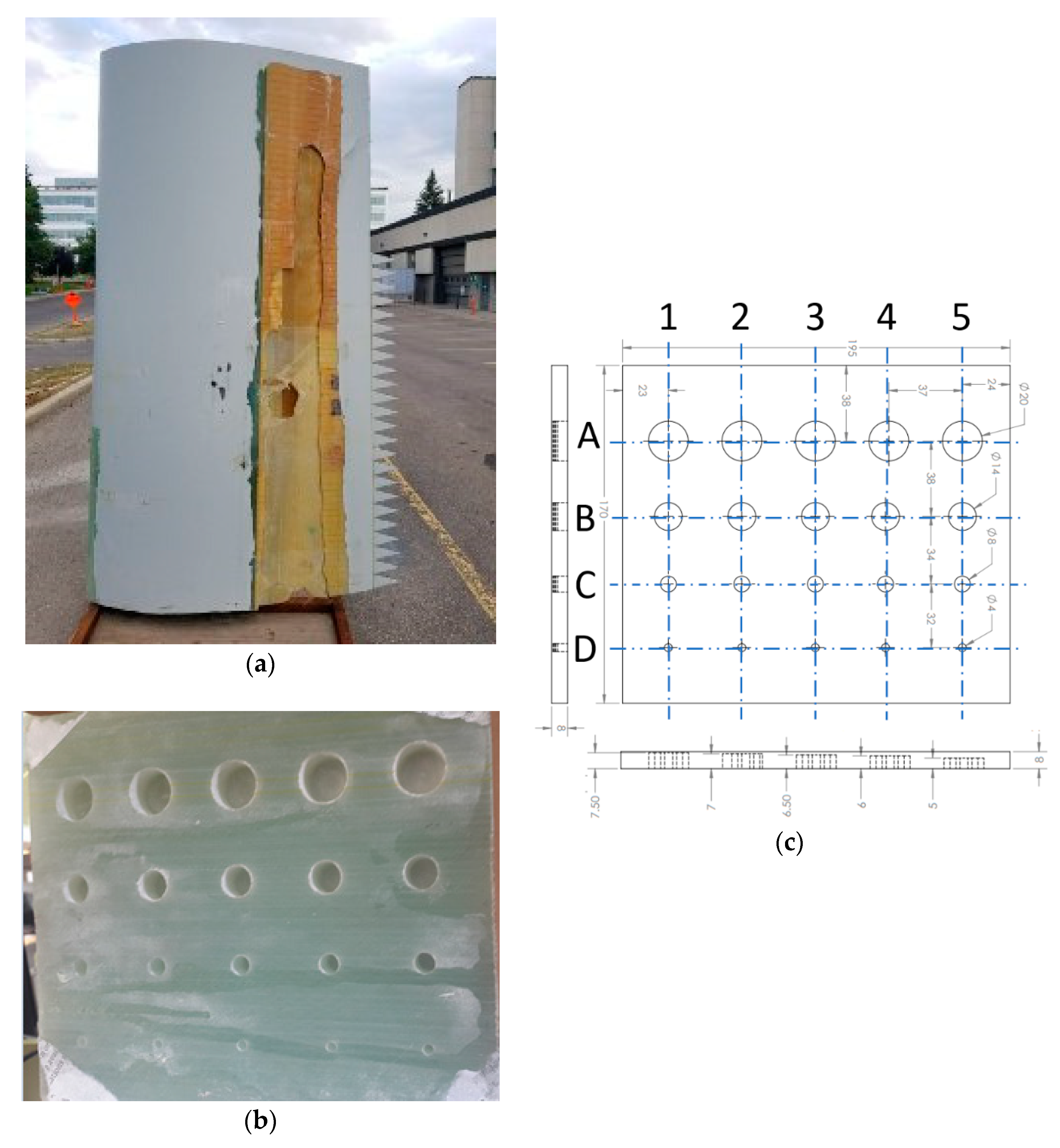
All samples used in this experiment came from a 50 m long wind turbine blade made of fiberglass composite obtained after it had been damaged in transit to a wind farm. The blade was never installed or operated. Figure 1a shows the 3 m long blade section with significant surface damage that was used for the passive thermography experiments. The laminate thickness in the damaged section was 14 mm. The chord length was approximately 1 m. The yellow/orange regions in Figure 1a are the exposed sandwich core on the rear section of the suction surface where there is very little laminate. Some patches of glue on the suction side resulted in different effusivity than the background and therefore generated spots with different brightnesses on the thermograms. The upper side of the blade section contained a crack which was visible to the naked eye.
A “defect plate” with dimensions of 170 mm × 195 mm × 8 mm was cut from the laminate skin of another section of the blade closer to the tip where the laminate skin was thinner. Flat-bottomed holes with different diameters and depths were drilled from the rear to produce a range of known “defects”. The holes had diameters ranging from 4 mm to 20 mm with depths between 0.5 mm and 3 mm. Figure 1c is a schematic of the plate that illustrates the geometry and pattern of the defects. No holes penetrated the outer surface of the plate which corresponded to the outer surface of a blade and all thermograms were of the outer surface. The defect plate was attached to the surface of the damaged blade section during passive thermography experimentation. It was also the only blade material tested with active thermography. The holes were used to evaluate the minimum defect that can be detected using passive and active thermography.
2.2. Passive Thermography
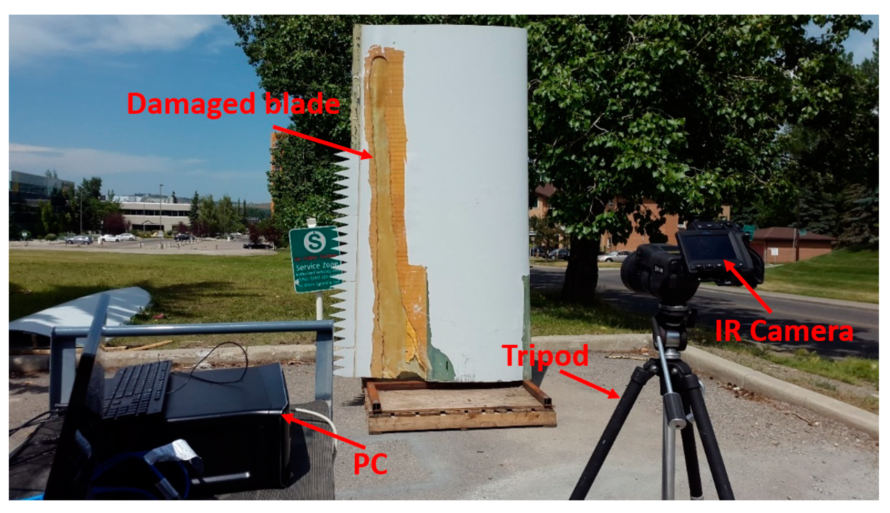
In the passive thermography experiment, the suction side of the blade was monitored outdoors during a sunny day from morning until the afternoon. The blade’s position was not changed relative to the IR camera during this time. This experiment, whose setup is depicted in Figure 2, sought to determine the most favorable conditions to reveal the most defects and to evaluate the fault detection capability of thermography when the blade is heated by the sun.
The experiment was conducted on a sunny day in July 2017 from 9:00 a.m. to 7:30 p.m. Sunrise and sunset on this day were 5:53 a.m. and 9:30 p.m., respectively. During the experiment, the sky was clear, the humidity was almost 36%, and the temperature varied between 16 °C and 26 °C. A T1030Sc IR camera made by FLIR Systems was located 4 m from the blade section and equipped with a 21.2 mm lens, resulting in a spatial resolution of 4 mm per pixel. ResearchIR, a software package developed by FLIR Systems that provides high-speed data recording and image analyzing capabilities was used to record thermograms at a frequency of 1 Hz.
2.3. Pulsed and Step Heating Thermography
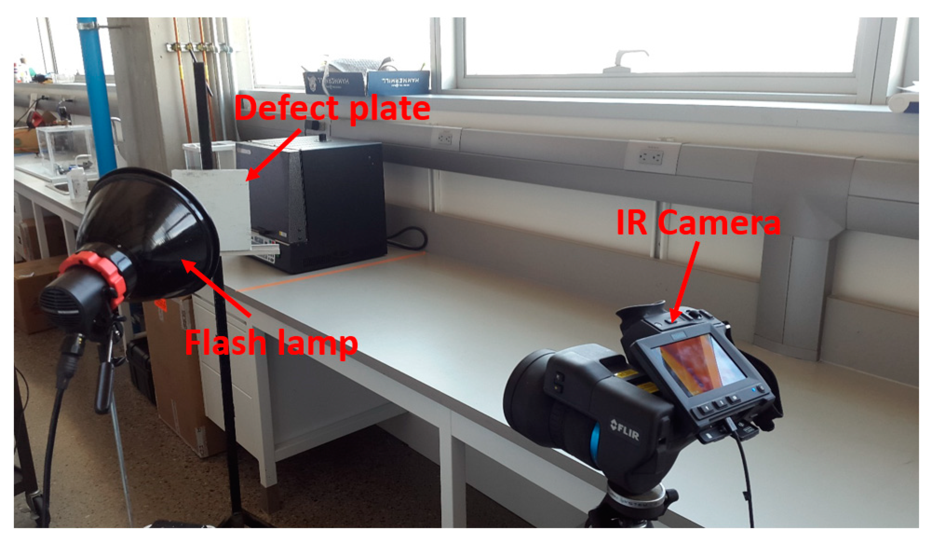
These techniques were used only on the defect plate mounted 1.5 m from the IR camera. Despite being mounted near windows, the defect plate was always in a shadow during the experiments. During pulsed thermography, the defect plate was heated by a 2400 W flash lamp and thermal images were recorded at a frequency of 15 Hz immediately after flashing the sample. To heat the surface uniformly, the flash lamp was around 0.3 m from the object with the angle of around 15° with respect to the normal of the defect plate. The pulsed thermography experiment is depicted in Figure 3. The spatial resolution of thermal images obtained by active thermography was almost 0.5 mm per pixel.
The step heating thermography experiment, shown in Figure 4, used two 500 W halogen lamps to continuously heat the surface. The sample was heated between 10 and 75 s and the thermal evolution on the surface of the specimen was recorded at a frequency of 15 Hz. Once heating was finished, thermal decay was recorded with the same frequency. The room temperature was 23 ± 2 °C during the experiment. The thermal contrast associated with the defects could be observed after a few seconds of heating.
3. MF Algorithms
MF is a method to improve image contrast of subsurface defects by increasing the contrast of defective areas and reducing the signals from sound areas [31,33,34]. Different types of MF algorithms have been developed, all of which are based on the assumption that [31,34]:
at any time. Tobs is the temperature recorded by the IR camera, Trefl is the temperature response reflected from the defective area, and Tideal is the ideal temperature response of the sound area. Equation (1) can be represented in vector form:
where these vectors collect all recordings over time and X = Tobs, S = Trefl, and W = Tideal. Equation (2) is multiplied by a vector q that maximizes the visibility of the reflected temperature from the defective area and minimizes the response of non-defective areas. The vector q can, therefore, be calculated by [31,34]:
where qT is the transpose of q. Different methods for finding q result in the different types of MF algorithms. Each MF algorithm considers a certain q vector to increase the contrast of defective areas and decrease the signals from sound areas. The q vector for the spectral angle map (SAM) is
where i and j imply that the calculation is repeated for all pixels of all thermal images to provide a single correlation image and ST. The adaptive coherence estimator (ACE) uses as q:
where C is covariance matrix of the ideal temperature vector defined as:
Tobs = Tref l = Tideal
X = S + W
The t- and F-statistics use the different q vectors to improve the contrast associated with defective areas:
and
where .
4. Quantitative Evaluation
The SNR of the images is a measure of the quality of data. The traditional definition of SNR is the ratio of the average magnitude of a signal to the magnitude of the background noise, determined as described in Section 5. If a distorted signal, y(n), is considered as:
where x(n) is a signal and is the background noise, the SNR can be written for N samples as [35]:
where |[x(n)]| is the magnitude of a signal and σ2 is the variance of the background noise. Since most signals have wide dynamic ranges, the SNR is usually given in decibels (dB), [36]:
where Δ is the peak value of the signal. Equation (11) can be simplified as:
5. Results and Discussion
The results of both the passive and active thermography are presented in this section. All temperatures were measured using the IR camera. The different image processing algorithms, employed to increase the quality of the thermal images, are described and their results are discussed in detail.
5.1. Active Thermography
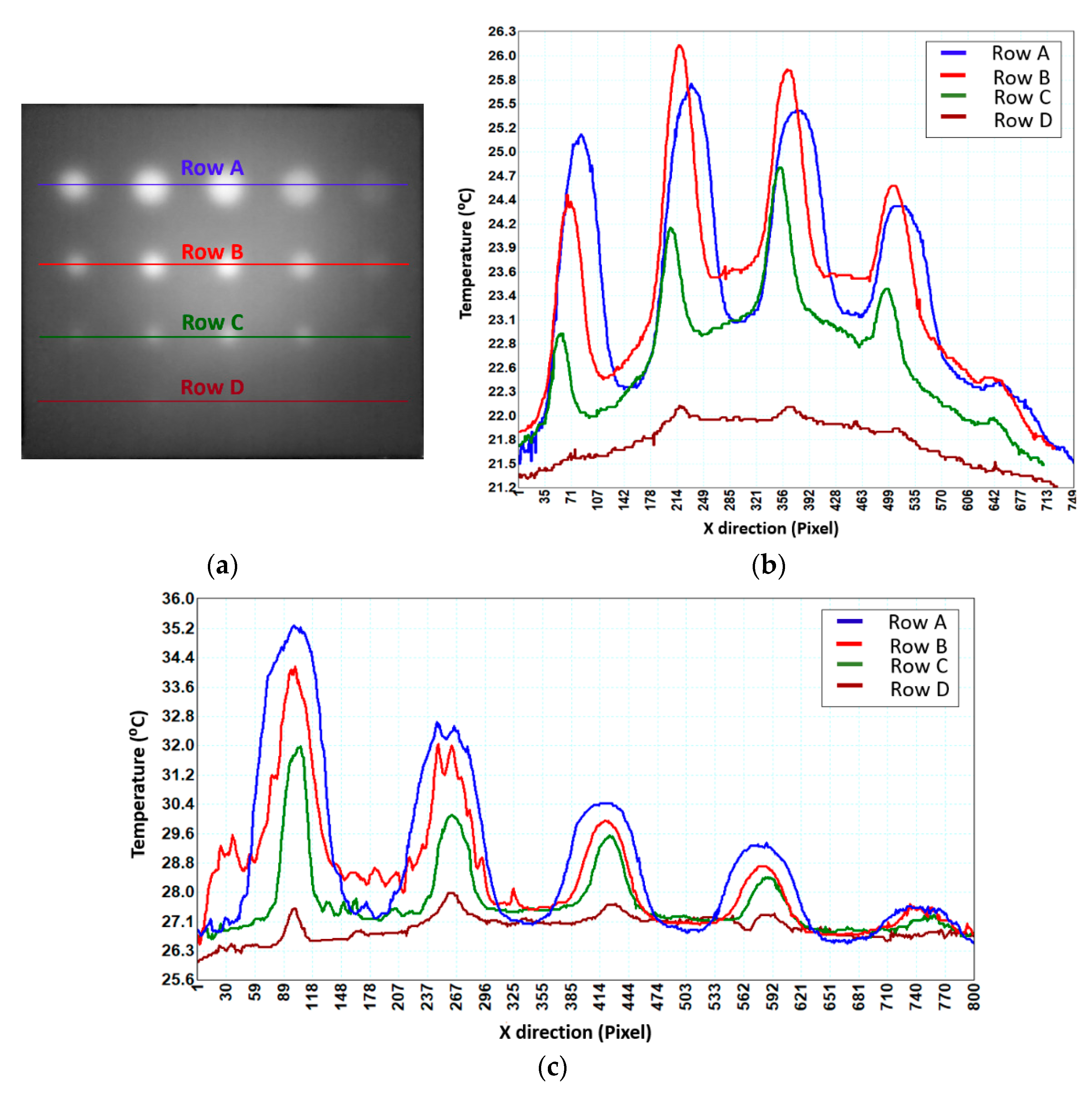
The temperature distribution profiles depicted in Figure 5b are plotted along with the rows identified in Figure 5a. The most visible contrasts of the defects revealed, as expected, that the deeper the defect, in terms of the distance from the bottom of the hole to the surface, the less detectable it was. Moreover, the size of the defect was important. The raw thermograms do not show smaller defects located deep within the plate. Defects with a diameter of 4 mm were barely detected. It can also be seen that the defects in the middle part of the plate are clearer than those towards the plate edges. This was primarily caused by non-uniform heating where the middle part of the sample received more thermal energy than the boundaries. The temperature distribution profiles during the step heating thermography for all pixels along the lines shown in Figure 5a are illustrated in Figure 5c. Figure 5c was recorded after heating for 75 s. The signals generated by the defects located in the last row, which have the smallest diameters, were not strong enough to be easily detected. Contrary to pulse thermography, Figure 5c shows that the surface of the object has been uniformly heated during the step heating thermography, which increased the efficiency of this method in detecting internal defects.
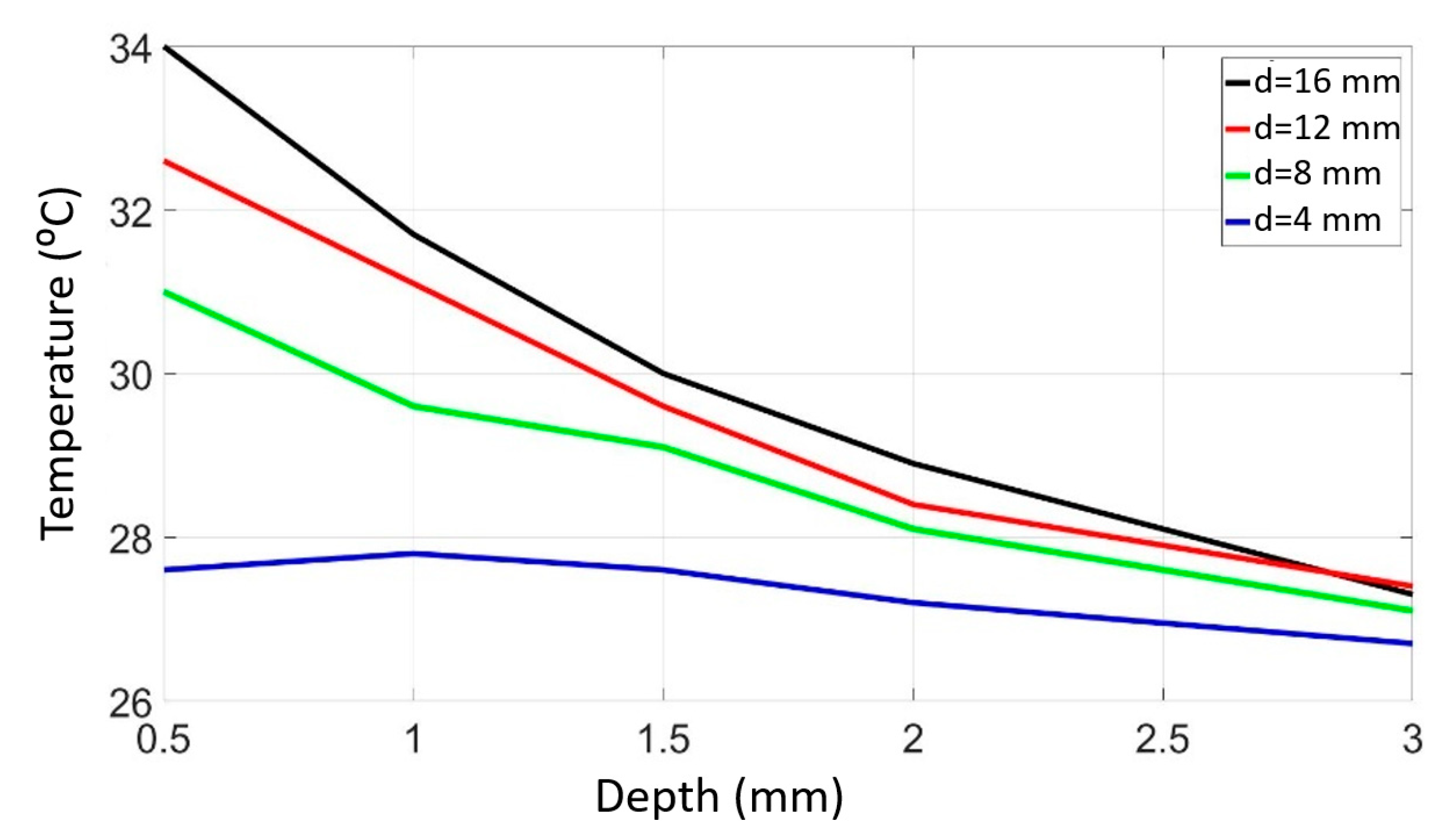
Temperatures near the defects were measured and analyzed to better evaluate the effects of the defect’s depth and size on the temperature variation. The temperatures measured at the locations of the flat-bottomed holes with various depths are illustrated in Figure 6. The sample was heated by two halogen lamps for 75 s, during which time data were recorded. It can be concluded from this figure that an increase in a defect’s depth reduces its temperature variation, which makes detection more difficult because there is not a significant change in the surrounding temperature.
By increasing the size of the defect, the slope of the temperature variation also increased, which implied that the effect of the depth variation on the temperature was more significant for larger defects.
The SNRs for the defect plate profiles shown in Figure 5a were determined to provide a quantitative evaluation of the detection. The signal values of the defects were measured first. The difference between the signal values of the defects and the background signals was identified as the peak value signal for the SNR calculation. Then, by calculating the standard deviation of the background noise and using Equation (12), the SNR of each defect was calculated. By comparing the visual results obtained from image processing and the corresponded SNR tables, defects with a SNR of more than almost three times the background noise was considered as a defect that can be identified by this method. The SNRs, related to raw thermal data captured by flash and step heating (heating and cooling periods) thermography, are listed in Table 1, Table 2 and Table 3. Defect position names used in these tables are defined in Figure 1c. It can be observed from these tables that bigger defects closer to the surface generated high SNRs. It can also be concluded from the results presented in these tables that raw thermograms of flash thermography can provide more details than step heating thermography. It should be noted that the SNRs of raw thermograms are compared later with values of the processed thermal images to show the strength of each of the image processing algorithms.
5.2. Image Processing and Quantitative Evaluation
The results for the fourth row in Figure 5 show that some subsurface defects cannot generate visible contrasts. This suggests the need for image processing to improve the resolution. Different algorithms, including MF, and a combination of PPT as a transform-based technique were employed to increase the SNR and the visibility of the defects. We will use the term “Step Phase and Amplitude Thermography” (SPAT) for the analysis of thermograms after heating and successfully used for passive thermal data processing.
5.2.1. Matched Filters (MF)
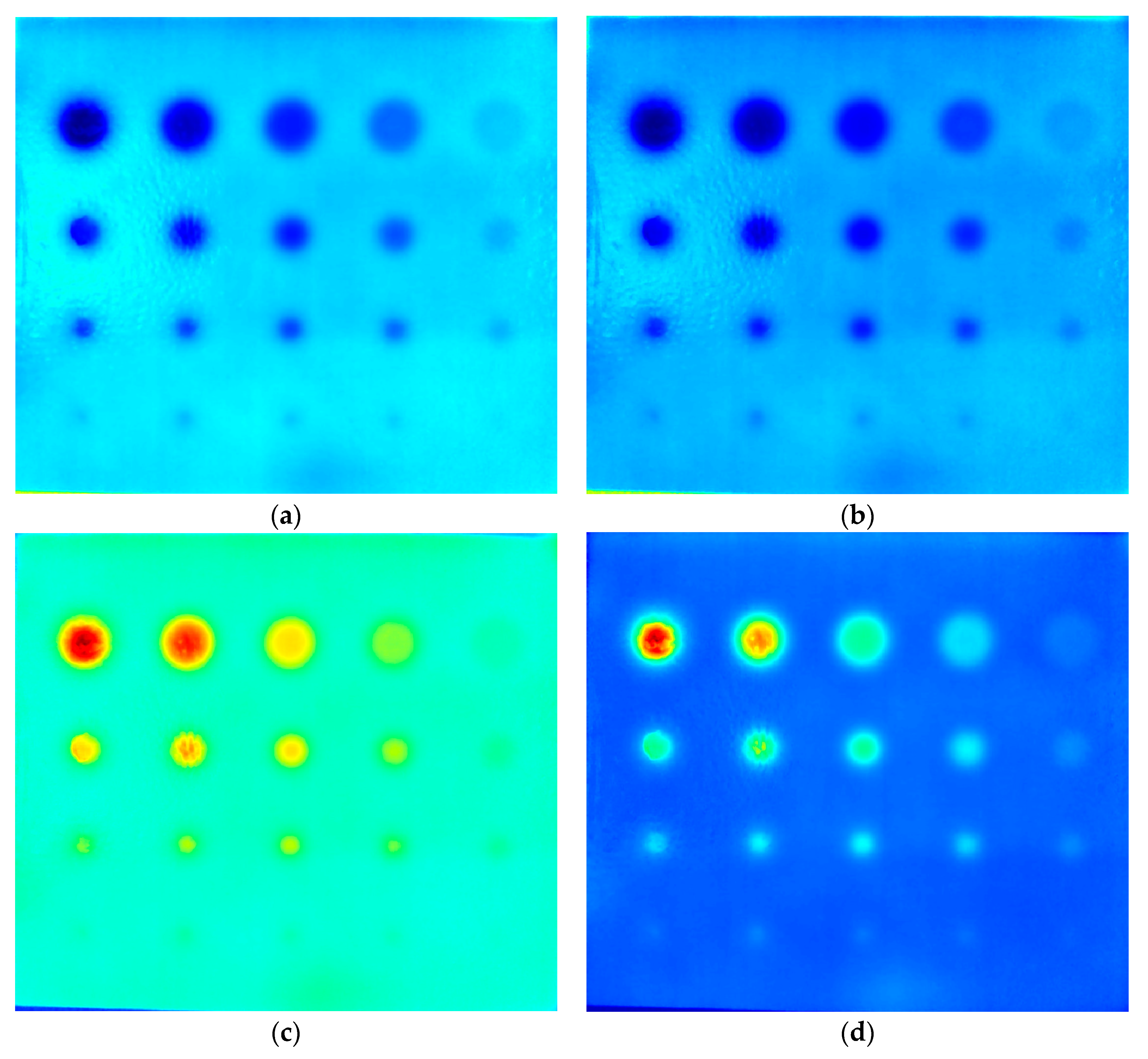
Applying MF to the step heating thermograms improved the quality of the results, as shown in Figure 7. All four versions of MF increased the visibility and contrast of the defects. Three of these filters, including the SAM, the ACE, and the F-statistic, showed very promising results where all defects could be detected. However, the t-statistic highly improved the quality of the raw thermal data and compared to other MF methods provided less details regarding subsurface defects.
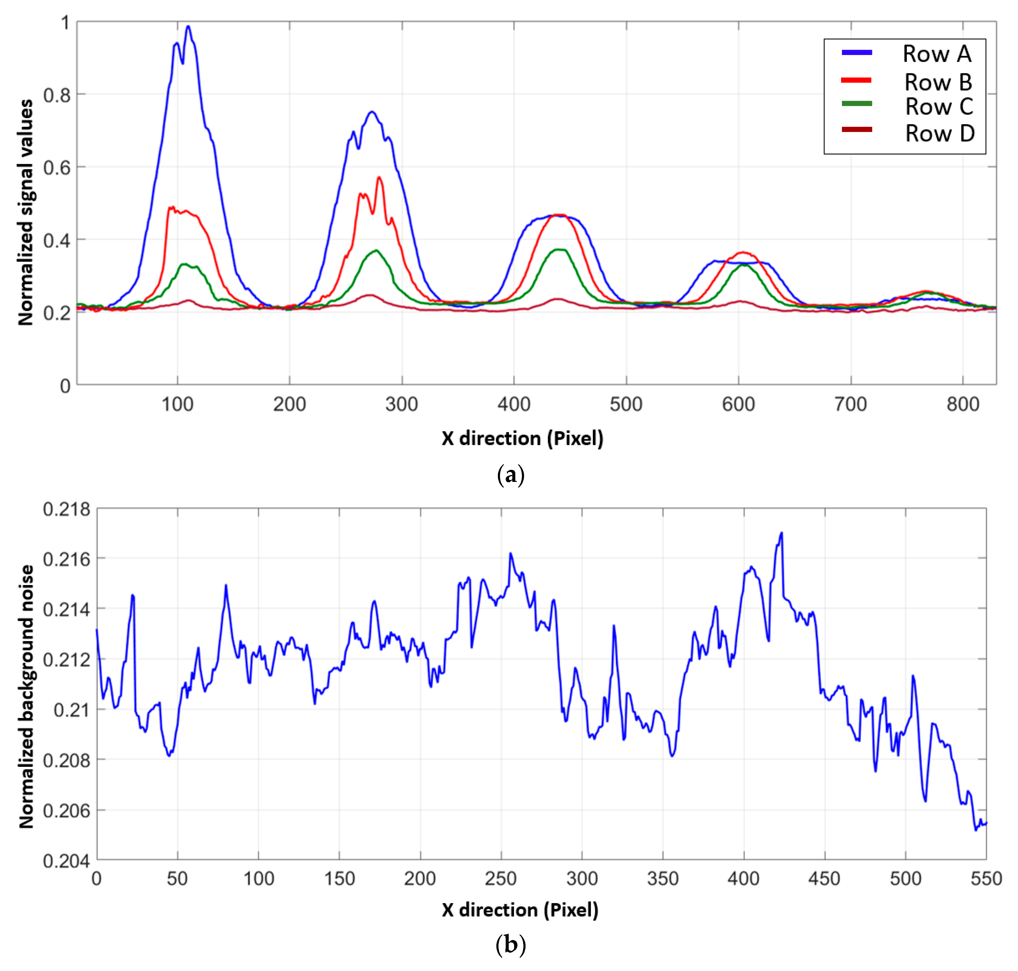
By using the above results, it can be seen that the diameter-to-depth ratio of the minimum detectable defect for each of SAM, ACE and F-statistic was 1.33, while this value for t-statistic was 2. To quantitatively evaluate the MF results, the SNRs for defective areas were determined. Figure 8a illustrates the signals of the F-statistic results obtained from the step heating data. The background noise around A2 is also shown in Figure 8b. These results were averaged to get the representative noise. It should be noted that all of the processed images have been normalized by dividing the intensity of each pixel over the difference between the maximum and minimum intensity available on the image.
The SNRs are presented in Table 4, Table 5, Table 6 and Table 7. The percentage improvement in the SNRs compared to the raw values is shown in parenthesis for each defect. These tables show that higher SNR values were obtained when MFs were applied to the step heating data. Therefore, the application of MFs to step heating data improved the resolution of the internal defects.
5.2.2. Transform-Based Techniques: Step Phase and Amplitude Thermography
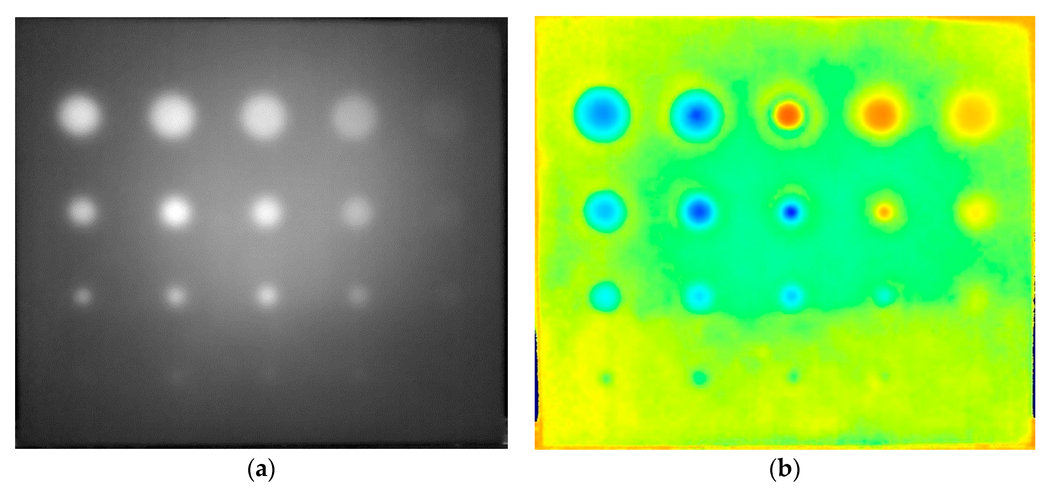
Pulsed thermograms were converted to a frequency domain using the FFT and the phase images were analyzed. Since the surface was excited uniformly during step heating, both phase and amplitude images of the transformed step heating thermograms were evaluated. Figure 9a,b shows a comparison of the raw pulsed thermograms and the normalized phase contrast obtained using the FFT. PPT significantly increased the contrast so that all defects, except D5, were detected. The same normalization method as the one used for the MF method was applied to the results obtained using the transformed-based techniques.
The SNR values for the phase images depicted in Figure 9 are presented in Table 8, which shows that larger defects that were closer to the surface had higher SNRs. The first column of defects is an exception to this observation, mainly due to non-uniform heating of the surface.
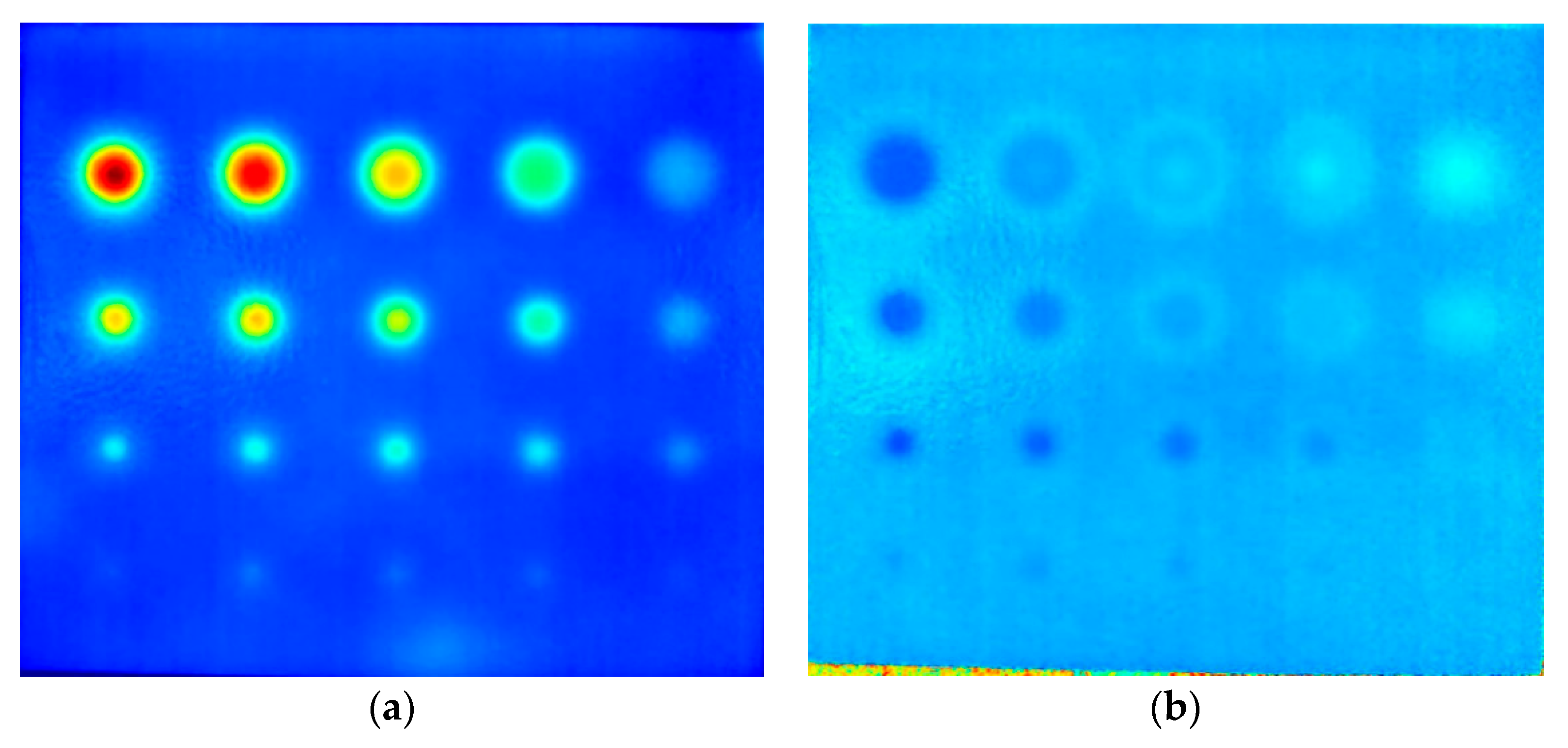
Figure 10a,b shows the phase and amplitude images at the minimum frequency where the FFT was applied to the step heating thermograms captured during cooling after heating for 75 s.
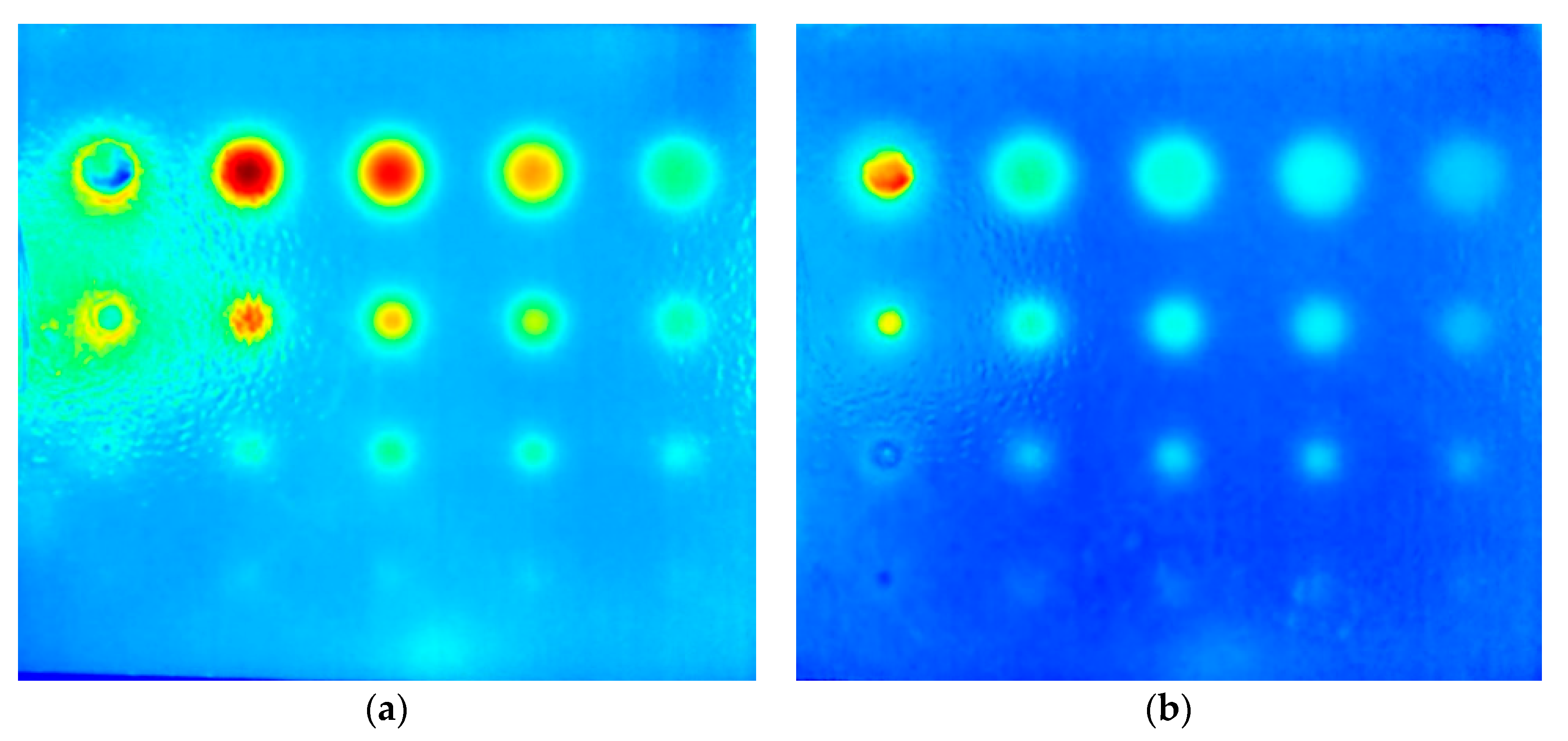
The diameter-to-depth ratio of the minimum detectable defect in each of phase images of PPT and SPAT was 2, while the amplitude of SPAT provided a better value of 1.33. It can be concluded from these results that the application of the FFT transform to step heating thermography was more effective than it was for flash thermography. This was especially true for the amplitude data, where clearer results with higher contrasts were achieved. Phase images revealed that defects with a better contrast compared to the amplitude images, in some cases. This demonstrated that a reliable inspection could be achieved by evaluating both results. Figure 11 shows the results of an FFT transform applied to thermograms captured during heating for 75 s. The phase image captured all defects—assumed to be indicated by the signals that were more than three times the background level—demonstrating that phase images extracted from the heating data provided more visibility compared to the data obtained from cooling. The amplitude images obtained during cooling were less noisy and contained more detail, which allowed the shape of defects to be determined.
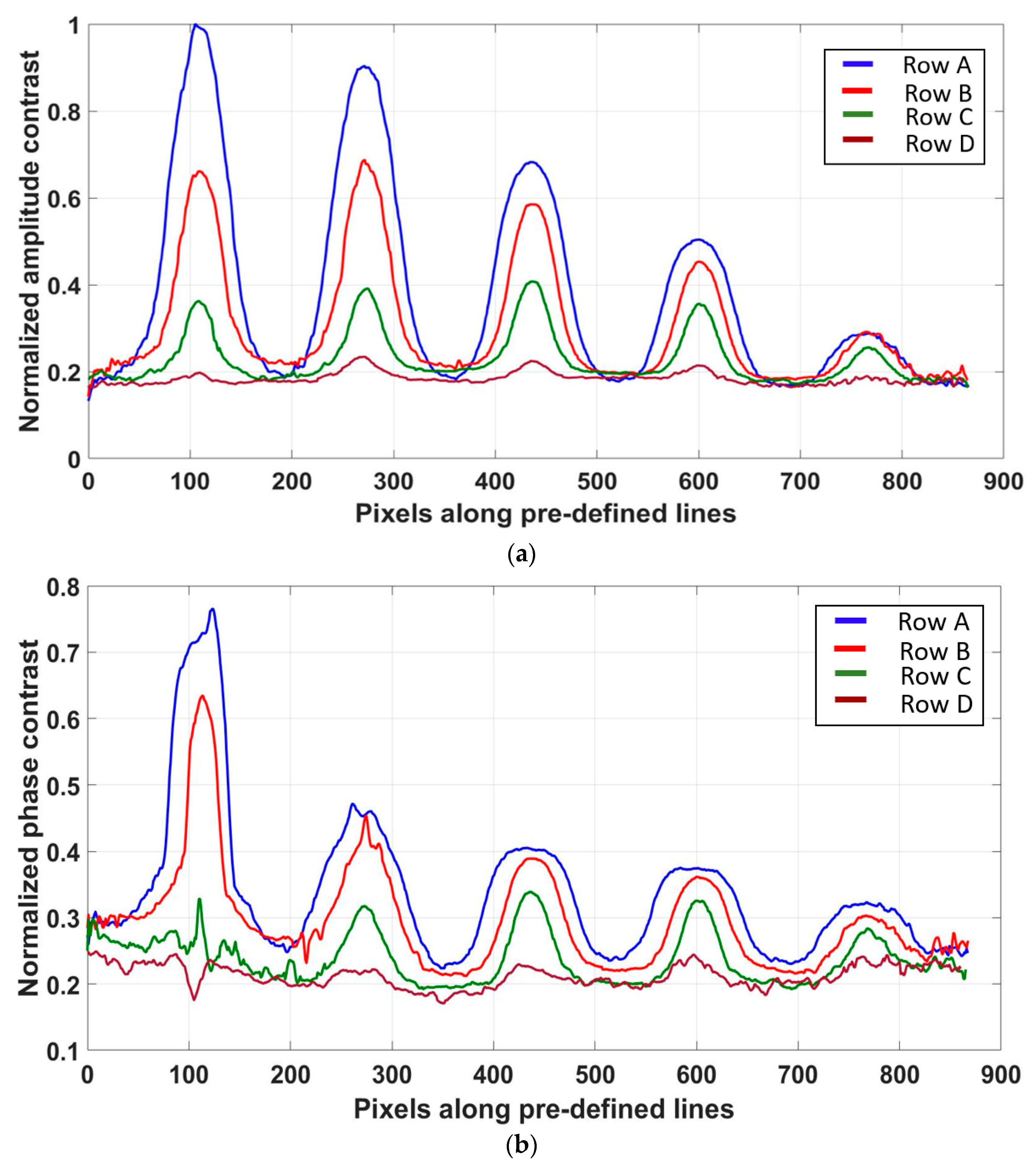
Figure 12a presents a further analysis of the normalized amplitude contrast distribution of the thermograms captured during cooling after 75 s of heating. The curves in this figure are the amplitude variation along the lines shown in Figure 5a. A significant change occurred between the sound and defective areas in the amplitudes, leading to a sharp boundary around the defects. The normalized phase contrast distribution of thermograms obtained after heating for 75 s is depicted in Figure 12b. Bigger defects closer to the surface generated higher phase contrasts and were subsequently more visible in the phase image. By analyzing these plots, all defects, except D5, on the defect plate were detected.
The SNR values for the phase and amplitude images captured by the application of FFT on the step heating data are listed in Table 9, Table 10 and Table 11. These results demonstrate that amplitude images extracted from thermal data captured during cooling had higher SNR values and revealed more details of subsurface defects. The SNRs of both the phase and amplitude images show that larger defects closer to the surface provided higher values.
By comparing the results presented in Table 8, Table 9, Table 10 and Table 11, it can be concluded from the results presented in Table 9, Table 10 and Table 11 that the application of the FFT transform to step heating thermography was more effective than its application to flash thermography. This was especially true for the amplitude data, where higher SNRs were achieved. The amplitude images extracted from step heating thermography were an effective means of revealing subsurface damage, as they detected even small and deep defects.
By comparing the results presented in Table 1, Table 2, Table 3, Table 4, Table 5, Table 6, Table 7, Table 8 and Table 9 related to the SNRs of raw and processed thermal data, it is concluded that the image processing algorithms significantly increased the visibility of subsurface defects especially those of smaller sizes, which are embedded in deeper areas.
5.3. Passive Thermography
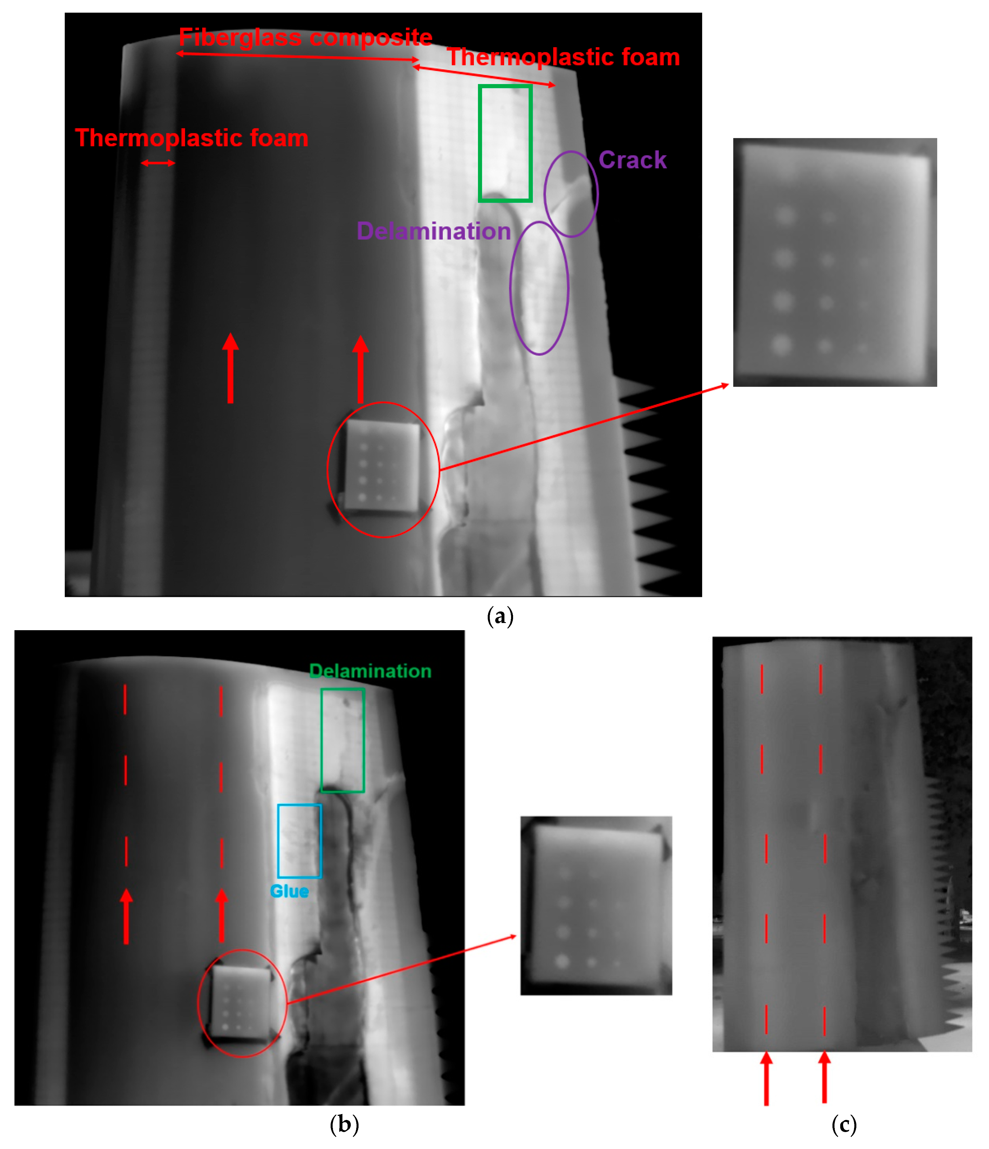
Passive thermal imaging of the damaged blade section was conducted at different times of the day. Typical results are shown in Figure 13. The results demonstrated that passive thermography was capable of capturing cracks, delamination, and internal features of the blade section.
Early morning experiments provided a visible contrast of the defects on the defect plate attached to the damaged blade section primarily due to the considerable temperature change on the blade during this period [2,18,19]. All defects in the plate, except the smallest 4 mm ones, were detected during this period. Less useful information about the defects was obtained when the experiment was performed around noon. None of the defects were visible during the evening (around 6 pm), which was mainly due to the balanced temperature on the blade surface after several hours of heating.
Thermal contrasts associated with dirt (glue on the surface), within the blue box in Figure 13, were most pronounced at noon. These contrasts faded during the afternoon. The blade’s internal features such as shear webs were detected as cold regions during the morning and at noon but became hot signatures during the evening after several hours of heating.
Cracks and delamination on the suction side were apparent near the blade’s trailing edge. At noon, with peak sunlight, cracks and delamination were detected. Delamination in the upper area, identified by the green box in Figure 13, were not detected clearly during the morning. The evening thermograms did not provide any information regarding cracks and delamination, so noon was the best time for crack and delamination monitoring.
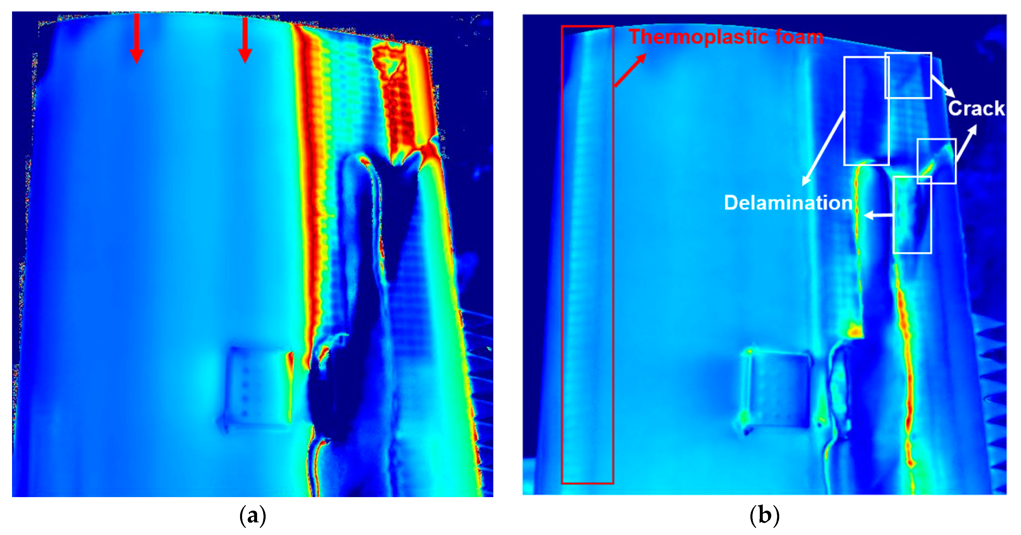
The transform-based technique, discussed in Section 5.2.2, SPAT, was employed for the first time to increase the quality of the passive thermography results. The phase images captured using this method were not sensitive to non-uniform heating. The FFT was applied to passive thermograms obtained at morning. The results are shown in Figure 14. Part (b) illustrates that the amplitude images considerably increased the quality and visibility of the visualized subsurface defects, as the visibility of cracks, delamination, and a large portion of the flat-bottomed hole defects was improved. Phase images have noticeably increased the contrast of shear webs signatures, marked by red arrows in Figure 14a.
Cracks and delamination are marked by white boxes in Figure 14b. The thermoplastic foam near the leading edge was detected in the amplitude results and is highlighted by the red box in Figure 14b. This method not only increased the quality of the thermal images and improved the detectability of thermography but also eliminated the false indications associated with environmental reflections, dirt, and dust on the surface.
6. Conclusions
The blades, the most critical components of wind turbines, are susceptible to failure due to initiation and propagation of subsurface damage in a number of forms. This study investigated thermography techniques for monitoring the condition of wind turbine blades. Active thermography, using pulsed and step heating, was conducted on a specially-constructed defect plate to evaluate this method’s potential for detecting subsurface defects. The 170 × 195 mm plate was cut from the laminate skin of a wind turbine blade. Flat-bottomed holes were drilled from the inside to produce “defects” with known diameters and penetrations. The results demonstrated that active thermography is a powerful method for the monitoring and fault detection of wind turbine blades but that the signals generated by some small defects could not be detected.
Passive thermography was conducted on a damaged blade section and attached defect plate. This experiment was conducted at different times of day to determine the most favorable time of a day for maximum defect detection. The results showed that early morning and noon were best for detecting certain types of defects. Cracks, delamination, and surface dirt generated the most visible signatures around noon, while defects such as flat-bottomed holes in the defect plate were more visible in the morning as the sun heated the targets. This conclusion applies to the day time experiments as there were not any overnight tests.
The raw thermograms obtained by both passive and active thermography could not reveal the small defects located deep in the laminate skin. Different image processing algorithms including Matched Filters, Thermal Signal Reconstruction, and Pulsed Phase Thermography were used to increase the quality of active thermograms. “Step Phase and Amplitude Thermography”, was used to analyze the step heating data. This technique gave the best detection of defects as measured by the diameter-to-depth ratio of 1.33. All the image processing algorithms improved the contrast in the active thermograms but some drawbacks can be considered for the Matched Filters method. The Matched Filters method is not fully automated and requires manual selection of points in a sound area of the damaged blade, which is time-consuming and affects the quality of results. In order to quantitatively evaluate the results, the signal-to-noise ratios of the raw and processed images were calculated. Higher ratios can be obtained when image processing algorithms are applied to the raw thermal data. As an obvious observation, larger defects closer to the surface generated higher ratios.
Step Phase and Amplitude Thermography, as a successful method for improving active thermography results, was applied to passive thermal data. The quality of passive thermograms was increased as a result. This method could also eliminate the false indications associated with environmental reflections and dirt on the surface. Nevertheless, it was not possible to resolve the smallest defects of 4 mm diameter whatever the depth. The minimum diameter-to-depth ratio for these defects was thus 1.25.
Author Contributions
The overall conception of this project was by D.W. and Q.S. who obtained the damaged wind turbine blade. The specific aims and implementation of them was done by H.S. as were all the experiments. All three authors contributed to writing the paper.
Funding
Hadi Sanati and David Wood acknowledge the Schulich endowment to the Faculty of Engineering, University of Calgary for providing funding for this work.
Conflicts of Interest
The authors declare no conflict of interest.
References
- Jüngert, A. Damage Detection in wind turbine blades using two different acoustic techniques. In Proceedings of the 7th fib PhD Symposium in Civil Engineering, Stuttgart, Germany, 10–13 September 2008. [Google Scholar]
- Meinlschmidt, P.; Aderhold, J. Thermographic inspection of rotor blades. In Proceedings of the 9th European Conference on NDT, Berlin, Germany, 25–29 September 2006. [Google Scholar]
- Tao, N.; Zeng, Z.; Feng, L.; Li, X.; Li, Y.; Zhang, C. The application of pulsed thermography in the inspection of wind turbine blades. In International Symposium on Photoelectronic Detection and Imaging 2011: Terahertz Wave Technologies and Applications; SPIE: Washington, DC, USA, 2011; p. 819319. [Google Scholar]
- Habali, S.M.; Saleh, I.A. Local design, testing and manufacturing of small mixed airfoil wind turbine blades of glass fiber reinforced plastics: Part II: Manufacturing of the blade and rotor. Energy Convers. Manag. 2000, 41, 281–298. [Google Scholar] [CrossRef]
- Lading, L.; Mcgugan, M.; Sendrup, P.; Rheinländer, J.; Rusborg, J. Fundamentals for Remote Structural Health Monitoring of Wind Turbine Blades—A Preproject Annex B—Sensors and Non-Destructive Testing Methods for Damage Detection in Wind Turbine Blades; Risø National Laboratory: Roskilde, Denmark, 2002. [Google Scholar]
- Rumsey, M.; Paquette, J. Structural health monitoring of wind turbine blades. Proc. SPIE 2008, 6933, 69330E. [Google Scholar]
- Schroeder, K.; Ecke, W.; Apitz, J.; Lembke, E. A fibre Bragg grating sensor system monitors operational load in a wind turbine rotor blade. Meas. Sci. Technol. 2006, 17, 1167. [Google Scholar]
- Liu, W.; Tang, B.; Jian, Y. Status and problems of wind turbine structural health monitoring techniques in China. Renew. Energy 2010, 35, 1414–1418. [Google Scholar] [CrossRef]
- Larsen, G.; Hansen, M.; Baumgart, A.; Carlén, I. Modal Analysis of Wind Turbine Blades; Risø National Laboratory: Roskilde, Denmark, 2002. [Google Scholar]
- Borum, K.; McGugan, M. Condition monitoring of wind turbine blades. In Proceedings of the 27th Riso International Symposium on Materials Science: Polymer Composite Materials for Wind Power Turbines, Roskilde, Denmark, 4–7 September 2006. [Google Scholar]
- Li, T.; Almond, D.P.; Rees, D.A.S. Crack imaging by scanning laser-line thermography and laser-spot thermography. Meas. Sci. Technol. Mar. 2011, 22, 35701. [Google Scholar] [Green Version]
- Pawar, S.S.; Peters, K. Through-the-thickness identification of impact damage in composite laminates through pulsed phase thermography. Meas. Sci. Technol. 2013, 24, 115601. [Google Scholar] [CrossRef]
- Maierhofer, C.; Myrach, P.; Reischel, M.; Steinfurth, H.; Röllig, M.; Kunert, M. Characterizing damage in CFRP structures using flash thermography in reflection and transmission configurations. Compos. Part B Eng. 2014, 57, 35–46. [Google Scholar]
- Maierhofer, C.; Arndt, R.; Röllig, M.; Rieck, C.; Walther, A.; Scheel, H.; Hillemeier, B. Application of impulse-thermography for non-destructive assessment of concrete structures. Cem. Concr. Compos. 2006, 28, 393–401. [Google Scholar] [CrossRef]
- Beattie, A.; Rumsey, M. Non-destructive evaluation of wind turbine blades using an infrared camera. In Proceedings of the 37th Aerospace Sciences Meeting and Exhibit, Reno, NV, USA, 11–14 January 1999. [Google Scholar]
- bin Zhao, S.; Zhang, C.; Wu, N. Infrared thermal wave nondestructive testing for rotor blades in wind turbine generators non-destructive evaluation and damage monitoring. In International Symposium on Photoelectronic Detection and Imaging 2009: Advances in Infrared Imaging and Applications; SPIE: Washington, DC, USA, 2009. [Google Scholar]
- Galleguillos, C.; Zorrilla, A.; Jimenez, A.; Diaz, L.; Montiano, Á.L.; Barroso, M.; Viguria, A.; Lasagni, F. Thermographic non-destructive inspection of wind turbine blades using unmanned aerial systems. Plast. Rubber Compos. 2015, 44, 98–103. [Google Scholar] [CrossRef]
- Worzewski, T.; Krankenhagen, R.; Doroshtnasir, M. Thermographic inspection of a wind turbine rotor blade segment utilizing natural conditions as excitation source, Part I: Solar excitation for detecting deep structures in GFRP. Infrared Phys. Technol. 2016, 76, 756–766. [Google Scholar] [CrossRef]
- Worzewski, T.; Krankenhagen, R. Thermographic inspection of wind turbine rotor blade segment utilizing natural conditions as excitation source, Part II: The effect of climatic conditions on thermographic inspections–A long term outdoor experiment. Infrared Phys. Technol. 2016, 76, 767–776. [Google Scholar] [CrossRef]
- Doroshtnasir, M.; Worzewski, T.; Krankenhagen, R.; Röllig, M. On-site inspection of potential defects in wind turbine rotor blades with thermography. Wind Energy 2016, 19, 1407–1422. [Google Scholar] [CrossRef]
- Lahiri, B.B.; Bagavathiappan, S.; Reshmi, P.R.; Philip, J.; Jayakumar, T.; Raj, B. Quantification of defects in composites and rubber materials using active thermography. Infrared Phys. Technol. 2012, 55, 191–199. [Google Scholar] [CrossRef]
- Shin, P.H.; Webb, S.C.; Peters, K.J. Pulsed phase thermography imaging of fatigue-loaded composite adhesively bonded joints. NDT E Int. 2016, 79, 7–16. [Google Scholar] [CrossRef] [Green Version]
- Maierhofer, C.; Röllig, M.; Krankenhagen, R.; Myrach, P. Comparison of quantitative defect characterization using pulse-phase and lock-in thermography. Appl. Opt. 2016, 55, D76–D86. [Google Scholar] [CrossRef] [PubMed]
- Almond, D.P.; Angioni, S.L.; Pickering, S.G. Long pulse excitation thermographic non-destructive evaluation. NDT E Int. 2017, 87, 7–14. [Google Scholar] [CrossRef]
- Maldague, X.; Marinetti, S. Pulse phase infrared thermography. J. Appl. Phys. 1996, 79, 2694–2698. [Google Scholar] [CrossRef] [Green Version]
- Chatterjee, K.; Tuli, S.; Pickering, S.; Almond, D. A comparison of the pulsed, lock-in and frequency modulated thermography nondestructive evaluation techniques. NDT E Int. 2011, 44, 655–667. [Google Scholar] [CrossRef] [Green Version]
- Montanini, M. Quantitative determination of subsurface defects in a reference specimen made of Plexiglas by means of lock-in and pulse phase infrared thermography. Infrared Phys. Technol. 2010, 53, 363–371. [Google Scholar] [CrossRef]
- Pawar, S.S. Identification of Impact Damage in Composite Laminates through Integrated Pulsed Phase Thermography and Embedded Thermal Sensors. Ph.D. Thesis, North Carolina State University, Raleigh, NC, USA, 2013. [Google Scholar]
- Ibarra, C.C. Quantitative Subsurface Defect Evaluation by Pulsed Phase Thermography: Depth Retrieval with the Phase. Ph.D. Thesis, Laval University, Quebec, QC, Canada, 2005. [Google Scholar]
- Shepard, S.M.; Lhota, J.R.; Rubadeux, B.A.; Wang, D.; Ahmed, T. Reconstruction and enhancement of active thermographic image sequences. Opt. Eng. 2003, 42, 1337. [Google Scholar] [CrossRef]
- Larsen, C. Document Flash Thermography. Master’s Thesis, Utah State University, Logan, UT, USA, 2011. [Google Scholar]
- Roche, J.M.; Balageas, D.L. Common tools for quantitative pulse and step-heating thermography—Part II: Experimental investigation. Quant. Infrared Thermogr. J. 2015, 12, 1–23. [Google Scholar] [CrossRef]
- Foy, B.R. Overview of Target Detection Algorithms for Hyperspectral Data; Rep. to NNSA, Rep. No. LU-UR-09-00593; Los Alamos Natl. Lab.: Los Alamos, NM, USA, 2009.
- Kretzmann, J. Evaluating the industrial application of non-destructive inspection of composites using transient thermography. Master’s Thesis, Stellenbosch Stellenbosch University, Stellenbosch, South Africa, 2016. [Google Scholar]
- Xia, X.G. A Quantitative Analysis of SNR in the Short-Time Fourier Transform Domain for Multicomponent Signals. IEEE Trans. Signal Process. 1998, 46, 200–203. [Google Scholar]
- Jain, J.; Jain, A. Displacement Measurement and Its Application in Interframe Image Coding. IEEE Trans. Commun. 1981, 29, 1799–1808. [Google Scholar] [CrossRef] [Green Version]
Figure 1.
(a) The damaged wind turbine blade. (b,c) The defect plate with flat-bottomed holes. All holes were drilled from the rear and did not penetrate the outer surface.
Figure 1.
(a) The damaged wind turbine blade. (b,c) The defect plate with flat-bottomed holes. All holes were drilled from the rear and did not penetrate the outer surface.

Figure 2.
Passive thermography experiment.

Figure 3.
Pulsed thermography experiment.

Figure 4.
Step heating thermography experiment.

Figure 5.
(a) Positions of temperature profiles. Temperature profiles using (b) pulsed and (c) step heating thermography. The rows are identified in (a).
Figure 5.
(a) Positions of temperature profiles. Temperature profiles using (b) pulsed and (c) step heating thermography. The rows are identified in (a).

Figure 6.
Effect of depth and size of the defect on the temperature distribution in a sample heated up by a halogen lamp for 75 s.
Figure 6.
Effect of depth and size of the defect on the temperature distribution in a sample heated up by a halogen lamp for 75 s.

Figure 7.
Four matched filters including (a) Spectral Angle Map (SAM), (b) Adaptive Coherence Estimator (ACE), (c) t-statistic and (d) F-statistic when the specimen was being step heated.
Figure 7.
Four matched filters including (a) Spectral Angle Map (SAM), (b) Adaptive Coherence Estimator (ACE), (c) t-statistic and (d) F-statistic when the specimen was being step heated.

Figure 8.
(a) Normalized signal values along the defect rows and (b) background noise around A2.

Figure 9.
(a) Raw thermogram and (b) phase image (acquisition time = 53.2 s) obtained from the thermal image sequence recorded during cooling after flashing the surface.
Figure 9.
(a) Raw thermogram and (b) phase image (acquisition time = 53.2 s) obtained from the thermal image sequence recorded during cooling after flashing the surface.

Figure 10.
(a) Amplitude image and (b) phase image of the thermograms captured during cooling after 75 s of heating.
Figure 10.
(a) Amplitude image and (b) phase image of the thermograms captured during cooling after 75 s of heating.

Figure 11.
(a) Amplitude image and (b) phase image of thermograms captured during heating for 75 s.

Figure 12.
(a) Normalized amplitude value and (b) normalized phase value distributions of the defects where the thermograms were obtained during cooling and heating, respectively.
Figure 12.
(a) Normalized amplitude value and (b) normalized phase value distributions of the defects where the thermograms were obtained during cooling and heating, respectively.

Figure 13.
(a) Thermographic results of the experiment around 9 a.m., (b) noon and (c) 6 p.m. (sunrise and sunset were around 5.53 a.m. and 9.30 p.m., respectively). The vertical arrows and dashed lines indicate the shear webs.
Figure 13.
(a) Thermographic results of the experiment around 9 a.m., (b) noon and (c) 6 p.m. (sunrise and sunset were around 5.53 a.m. and 9.30 p.m., respectively). The vertical arrows and dashed lines indicate the shear webs.

Figure 14.
(a) Phase images of the passive thermograms captured during the morning at a frequency of 0.00184 Hz and (b) amplitude image of the passive thermograms recorded during the morning at a frequency of 0.0165 Hz.
Figure 14.
(a) Phase images of the passive thermograms captured during the morning at a frequency of 0.00184 Hz and (b) amplitude image of the passive thermograms recorded during the morning at a frequency of 0.0165 Hz.


Table 1.
Signal to Noise Ratio (SNR) (dB) related to raw data captured by step heating thermography (heating period).
Table 1.
Signal to Noise Ratio (SNR) (dB) related to raw data captured by step heating thermography (heating period).
| 1 | 2 | 3 | 4 | 5 | |
|---|---|---|---|---|---|
| A | 18.4 | 18.2 | 17.8 | 14.4 | 3 |
| B | 18.1 | 18 | 17.7 | 12.9 | 6 |
| C | 17.9 | 17.5 | 17 | 11 | NA |
| D | 12.3 | 12 | 8.6 | NA | NA |
Table 2.
SNR related to raw data captured by step heating thermography (cooling period).
| 1 | 2 | 3 | 4 | 5 | |
|---|---|---|---|---|---|
| A | 25.7 | 24.9 | 22.8 | 19.4 | 12.3 |
| B | 24.4 | 20 | 20.4 | 17.5 | 11.9 |
| C | 7.4 | 10.2 | 15.2 | 11.5 | 5.9 |
| D | NA | 2.58 | 2.5 | NA | NA |
Table 3.
SNR related to raw data captured by flash thermography.
| 1 | 2 | 3 | 4 | 5 | |
|---|---|---|---|---|---|
| A | 16.3 | 18.5 | 18.5 | 13.7 | 3.4 |
| B | 10.2 | 15.8 | 17 | 11.9 | 2.9 |
| C | 2.5 | 4.2 | 13.1 | 4.9 | 2.6 |
| D | NA | 2.1 | 2.3 | 2.1 | NA |
Table 4.
SNR (dB) for SAM on step heating thermal data.
| 1 | 2 | 3 | 4 | 5 | |
|---|---|---|---|---|---|
| A | 36.8 (99%) | 35.3 (94%) | 31.8 (78%) | 26.9 (87%) | 15.1 (396%) |
| B | 33.5 (84%) | 33.7 (87%) | 31.2 (76%) | 27.9 (116%) | 17 (185%) |
| C | 30.7 (72%) | 29.3 (67%) | 29.1 (70%) | 26.3 (139%) | 18.8 |
| D | 16.1 (31%) | 18.7 (55%) | 18.6 (116%) | 13.9 | 5.5 |
Table 5.
SNR (dB) for ACE on step heating thermal data.
| 1 | 2 | 3 | 4 | 5 | |
|---|---|---|---|---|---|
| A | 33.2 (79%) | 31.9 (76%) | 29.1 (63%) | 24.3 (68%) | 11.6 (282%) |
| B | 30.6 (68%) | 29.9 (66%) | 28.5 (60%) | 25.4 (97%) | 15.3 (185%) |
| C | 26.4 (48%) | 27.1 (54%) | 26.5 (55%) | 24 (118%) | 16.7 |
| D | 14.7 (19%) | 16.9 (40%) | 16.9 (96%) | 11.7 | 8.5 |
Table 6.
SNR (dB) for the t-statistic on step heating thermal data.
| 1 | 2 | 3 | 4 | 5 | |
|---|---|---|---|---|---|
| A | 44.3 (139%) | 41.6 (129%) | 34.9 (95%) | 28.5 (90%) | 15.7 (416%) |
| B | 35.6 (95%) | 37 (105%) | 34.5 (95%) | 38.8 (201%) | 22.7 (280%) |
| C | 28.2 (58%) | 30.2 (72%) | 30.3 (77%) | 27.6 (151%) | 19.4 |
| D | 13.5 (10%) | 18.4 (53%) | 16 (85%) | 11.3 | 6.6 |
Table 7.
SNR (dB) for the F-statistic on step heating thermal data.
| 1 | 2 | 3 | 4 | 5 | |
|---|---|---|---|---|---|
| A | 40.2 (117%) | 37.6 (107%) | 32.7 (83%) | 27 (87%) | 13.8 (354%) |
| B | 33 (82%) | 33.8 (88%) | 32.2 (82%) | 28.3 (120%) | 17.8 (198%) |
| C | 27.2 (52%) | 28.9 (65%) | 28.6 (68%) | 26.1 (137%) | 18.5 |
| D | 13.5 (10%) | 17.2 (44%) | 16.5 (92%) | 11.6 | 2.7 |
Table 8.
SNR (dB) for Pulsed Phase Thermography (PPT) data.
| 1 | 2 | 3 | 4 | 5 | |
|---|---|---|---|---|---|
| A | 25.5 (56%) | 26.8 (45%) | 24.9 (35%) | 23.2 (69%) | 20.7 (511%) |
| B | 23.1 (127%) | 26.5 (67%) | 26.9 (58%) | 23.4 (96%) | 19.9 (591%) |
| C | 19.6 (677%) | 20.8 (397%) | 19.8 (52%) | 14.2 (190%) | 12.9 (401%) |
| D | 13.9 | 16.4 | 12.8 | 7 (234%) | NA |
Table 9.
SNR (dB) of amplitude image captured during cooling after 75 s heating.
| 1 | 2 | 3 | 4 | 5 | |
|---|---|---|---|---|---|
| A | 46.2 (80%) | 45.1 (81%) | 42.2 (85%) | 38.4 (98%) | 29.7 (141%) |
| B | 41 (68%) | 41.3 (106%) | 39.6 (94%) | 36.7 (109%) | 28.7 (140%) |
| C | 33.1 (349%) | 33.7 (231%) | 34.6 (128%) | 33.4 (190%) | 25.9 (338%) |
| D | 14.9 | 23.5 (809%) | 21.2 (763%) | 17 | 13.6 |
Table 10.
SNR (dB) of phase image captured during 75 s heating.
| 1 | 2 | 3 | 4 | 5 | |
|---|---|---|---|---|---|
| A | 38.5 (183%) | 30.9 (144%) | 29.2 (127%) | 27.6 (180%) | 23.6 (774%) |
| B | 36 (302%) | 32 (160%) | 29.2 (132%) | 27.5 (208%) | 23.2 (896%) |
| C | 21.5 (1211%) | 26.3 (707%) | 27.8 (164%) | 26.6 (580%) | 22.9 (907%) |
| D | 19 | 13.3 (1044%) | 18.3 (827%) | 17.7 (710%) | 12.7 |
Table 11.
SNR (dB) of amplitude image captured during 75 s heating.
| 1 | 2 | 3 | 4 | 5 | |
|---|---|---|---|---|---|
| A | 33.6 (106%) | 41.9 (127%) | 40.8 (120%) | 38.3 (179%) | 31.6 (834%) |
| B | 26.9 (163%) | 38.5 (142%) | 37.6 (121%) | 34.7 (191%) | 29.2 (915%) |
| C | 20.3 (706%) | 26.2 (527%) | 30.1 (130%) | 28.7 (484%) | 24.2 (842%) |
| D | 8 | 13.1 (537%) | 12.7 (455%) | 10.8 (416%) | 9.4 |
© 2018 by the authors. Licensee MDPI, Basel, Switzerland. This article is an open access article distributed under the terms and conditions of the Creative Commons Attribution (CC BY) license (http://creativecommons.org/licenses/by/4.0/).
Share and Cite
MDPI and ACS Style
Sanati, H.; Wood, D.; Sun, Q. Condition Monitoring of Wind Turbine Blades Using Active and Passive Thermography. Appl. Sci. 2018, 8, 2004. https://0-doi-org.brum.beds.ac.uk/10.3390/app8102004
AMA Style
Sanati H, Wood D, Sun Q. Condition Monitoring of Wind Turbine Blades Using Active and Passive Thermography. Applied Sciences. 2018; 8(10):2004. https://0-doi-org.brum.beds.ac.uk/10.3390/app8102004
Chicago/Turabian StyleSanati, Hadi, David Wood, and Qiao Sun. 2018. "Condition Monitoring of Wind Turbine Blades Using Active and Passive Thermography" Applied Sciences 8, no. 10: 2004. https://0-doi-org.brum.beds.ac.uk/10.3390/app8102004
Note that from the first issue of 2016, this journal uses article numbers instead of page numbers. See further details here.