Seabed Sediment as an Annually Renewable Heat Source


1
School of Technology and Innovations, University of Vaasa, P.O. Box 700, FI-65101 Vaasa, Finland
2
Geo-Pipe GP Oy, Konsterinkuja 5, FI-65280 Vaasa, Finland
*
Author to whom correspondence should be addressed.
Appl. Sci. 2018, 8(2), 290; https://0-doi-org.brum.beds.ac.uk/10.3390/app8020290
Submission received: 15 December 2017
/
Revised: 1 February 2018
/
Accepted: 9 February 2018
/
Published: 15 February 2018
(This article belongs to the Special Issue New Heating and Cooling Concepts)
Abstract
:Thermal energy collected from the sediment layer under a water body has been suggested for use as a renewable heat source for a low energy network. A prototype system for using this sediment energy was installed in Suvilahti, Vaasa, in 2008 and is still in use. It provides a carbon-free heating and cooling solution as well as savings in energy costs for 42 houses. To be a real, renewable heat source, the thermal energy of the sediment layer needs to replenish annually. The goal of this paper is to verify the possible cooling or annual heat regeneration. The sediment temperatures were measured and analyzed in the years 2013–2015. The data were compared to the same period in 2008–2009. All measurements were taken in the same place. This paper also confirms the potential of the sediment heat, especially in the seabed sediment, using the temperature differences between the lowest and the highest values for the year. The results demonstrate that the collection of the heat energy does not cause permanent cooling of the sediment. This result was obtained by calculating the temperature difference between measurements in the warmest month and the month with the coldest temperatures. This indicates the extracted energy. The difference was found to be around 9.5 °C in 2008–2009, rising to around 11 °C for the years 2013–2014 and 2014–2015. This indicates the loaded energy. The energy utilization is sustainable: the sediment temperature has not permanently decreased despite the full use of the network for the heating and cooling of houses between 2008 and 2015.
1. Introduction
The limited resources of non-renewable energy, the prevention of climate change and environmental issues like UHI (urban heat island) effect are the concerns that make the search for renewable energy sources important. One of the research topics is geothermal energy. In non-volcanic areas, geothermal energy plays a minor role compared to the radiant energy of the Sun, which has accumulated in the topmost layers of the ground. The term ‘geoenergy’ consists of both geothermal energy from the Earth and the radiant energy of the Sun. Geoenergy is available, for example, in ground, bedrock, watercourses, in sediment under water bodies and under asphalt and concrete surfaces. In Finland, the most exploited forms of geoenergy are ground source heat and bedrock heat.
The new renewable energy sources, such as sediment heat under water bodies and asphalt heat under the surfaces of roads and parking lots, are today attracting great interest. Sediment heat can be harvested from the sediment layers at the bottom of different watercourses. Sediment is a solid-state layer consisting of clay, mud and gyttja. There are thick sand layers on the coastline of Finland and plenty of sediment in shallow bays. According to Likens and Johnson [1], the temperature variations in overlying water and the thermal properties of the sediment affect the heat budget of the sediments. In their study, a thermistor and a resistance bridge were used in the temperature measurements on sites in Wisconsin. Golosov and Kirillin [2] stated that the thermal effect of the sediments on the lake water temperature is observable in shallow lakes. They also noticed that in seasonally ice-covered lakes the sediment is the major heat source influencing the ecology, e.g., oxygen consumption and nutrients supply. Considering the sea bay conditions, the extraction of heat energy does not appear to be affecting the ecosystem.
In 2006, it was observed in Ostrobothnia, Finland, that at a depth of three meters under the water body of lakes the temperature of sediment reached 8 °C and remained quite stable (8–9 °C) in deeper layers.
In the same year, the interest in renewable seabed sediment heat energy arose in Vaasa in Western Finland too. The location where the heat was first noticed was in Suvilahti Bay. The elevated temperatures were verified by the Geological Survey of Finland, which performed temperature and resistance measurements at three different points on April 11. Following this discovery, the temperatures of sediment were researched as point measurements in many waterways in Ostrobothnia and, according to private communications with the Geological Survey of Finland, it was noticed that there was potential for heat energy at the bottom of lakes and also the sea.
Due to previous results, which confirmed the discovery of the promising heat resource, two years later, the low energy network for seabed sediment was introduced in the Vaasa House Fair area of Suvilahti. The Vaasa House Fair area was situated close to the seashore and sediment in the area was found to consist of sulfide clay mud. The long-term average air temperature in Vaasa is −5.7 °C in winter and 14.9 °C in summer [3].
In our previous papers we have found out that the calculated annual loaded seabed sediment heat energy of 7800 m heat collection pipeline is 575 MWh. Meanwhile the annual extraction of energy in such low energy network is 560 MWh [4].
The goal of the present study is to verify the adequacy of this heat resource for continuous heating of houses. The paper will identify the potential of sediment heat, especially in seabed sediment, using the temperature differences between the lowest and the highest values. Measurements of sediment temperatures were taken in a residential area that utilizes the sediment heat-based low energy network. One focus is to ascertain whether the usage of the low energy network has caused permanent temperature changes in the sediment. At the same time, it is essential to annually investigate the principle of the heat loading and unloading: for how many months are the temperatures increasing each year and for how many months are they decreasing each year? One of the major issues in the utilization of sediment energy is the availability and sustainability of heat energy.
2. Thermal Interaction between Water and Sediment
The use of sediment thermal energy for heating is based on the annual recharge of the thermal energy in sediments. This recharging is mainly caused by an interaction between water and sediment. Of course, water and sediment interact in many ways. Here, the focus is on the thermal interaction when water is either brine or fresh water. The main feature affecting the thermal energy of sediments is the temperature of the overlaying body of water when there is no tide. Birge et al. [5] carried out one of the first studies of this feature as early as 1927 at Lake Mendota where the heat exchange of mud was measured at different water depths but with sediments within the thickness of five meters. Birge et al. noted a variation in the migration rate of the heat. They showed that the annual oscillation at the sediment temperature attenuates as a function of increasing depth. In a study conducted at Indian River on the Atlantic Coast of Florida in the 1980s, Smith [6] also reported results that show that the water column and underlying sediments have an active exchange of heat.
Many publications indicate that the heat exchange between the water body and the lake sediments cannot be ignored, especially when a lake is shallow or has an ice cover for some period of the year [7,8,9,10]. The role of sediment in transferring the stored heat back to the water body during winter has been investigated in the arctic lakes, for example by Welch and Bergmann [9]. According to Bengtsson [11], the heat flow from the sediments happened during the whole of winter but the convective mixing was very slow.
The sediment heat flux is a signification parameter when simulating the stratification conditions in shallow lakes but not in deeper lakes [10]. A study of dynamic heat exchange in the sediment-water interface of a lake indicates the same conclusion: Fang and Stefan [12] noted that the sediment heat fluxes are a very important factor in shallow lakes. The lake sediments provide seasonal heat storage and thermal inertia to water columns. The direction of the heat flux has both seasonal and daily variations. Seasonal variation causes heat transfer from water to sediment in the summer and from sediment to water in the winter.
Brewer [13] studied shallow lakes with depths approximately between 0.5–1.0 m and 1.8–2.7 m in the Barrow area of Alaska. He stated that during the ice-free period, the water in the lake can be considered to be in an isothermal state with a maximum recorded temperature of 12 °C. Following the icing of the lake surface, the heat radiation through the ice can quickly warm the water, even from approximately 0 °C to 2 °C, as long as the ice is not covered by snow. The snow on the ice causes the cooling of the water and then the bottom sediments start to warm the water. Warming depends on the distance from the shore and the depth of the water body.
A great deal of heat energy is available in urban areas. Buildings and surface materials, such as concrete and asphalt pavements, absorb and store sunlight effectively; together, the built environment, people, vehicles and lack of flora are the reasons for the extra heat [14]. This phenomenon, referred to as the urban heat island (UHI) effect, is largely noticed in big cities. The air in an urban area is warmer than that in the nearby rural area. The difference may even be several degrees [15]. In Turku, Finland, the average UHI intensity has been measured as 1.9 °C and the periodic difference between temperatures in the city center and surrounding areas have risen up to 10 °C [16]. The UHI effect also has an influence on ground and water temperatures. There are many different kinds of water courses, bottom sediment and heat beneath urban areas and these can be utilized as low energy sources for buildings. In their research, Canbing, Jincheng and Yijia concluded that the urban heat island effect feeds itself [17]. Thus, the best energy-saving potential can be reached by mitigating the UHI effect. Santamouris [18] also sees the use of energy supply systems that utilize renewable energy sources for buildings, as one solution in the battle against urban warming.
3. Materials and Methods
The House Fair was arranged in Suvilahti, Vaasa in the summer of 2008. The themes of the Fair were homes for everyone and ecology. The energy solutions for the area were based on renewable energy. The heating and cooling energy for 42 detached houses was delivered from the seabed sediment. This energy was mainly produced by the Sun. The combined heat and power plant, which utilizes the biogas of the landfill, was also built in the area. The combined heat and power (CHP) station produced electricity to the heat pumps of the low energy network. The House Fair Area of Vaasa and its unique low energy network were thoroughly described by Hiltunen et al. [19].
The temperatures of the seabed sediment can be measured from two places on the shore. Immediately after the assembling process in 2008, the temperatures were measured once a month for a period of 13 months using the optical cables of the distributed temperature sensing method (DTS). The measurements were carried out by the Geological Survey of Finland with the help of Agilent N4386A and had a temperature accuracy of ±0.17 °C. In 2013–2015, the University of Vaasa recorded the sediment temperature measurements. The measurements were taken once a month with the help of the Sensornet Oryx DTS device. The temperature accuracy of the DTS device was ±0.5 °C. The sediment temperatures were measured by utilizing the same methods as those noted earlier. The results were obtained from a distance of 0–300 m, starting from the shore. The spatial resolution of the measurements was 1 m. The final sediment temperatures were acquired as an average of eight temperatures measured on the same day during a period of around ten minutes.
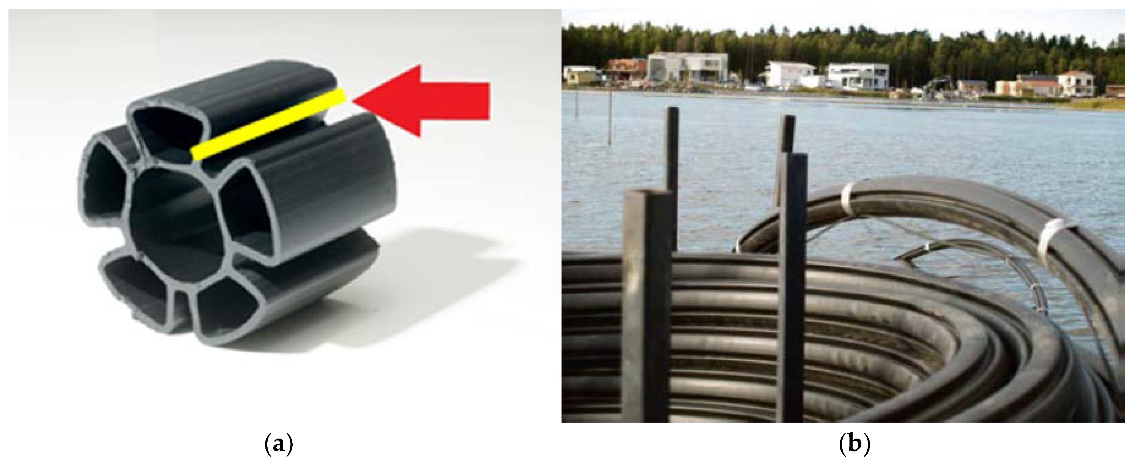
The optical cables for temperature measurements were installed at the same time as the assembly process of the collector pipes. The position of an optical cable (yellow line) is shown in Figure 1a.
The present study is concerned with the temperatures measured in Liito-oravankatu in the Suvilahti suburb during six-month periods in 2013–2014 and 2014–2015. The temperatures for those periods were compared with results from the corresponding months in 2008–2009 to illustrate the cooling period in the sediment layer. The measurements were taken in the same place in each period of 2008–2009, 2013–2014 and 2014–2015. In addition to these results, the warming of the sediment layer is also presented for the respective years.
Data are also available for the temperatures of the heat carrier fluid measured by a resident of one single-family house in the low energy network area in Suvilahti. Using an Ouman thermistor, the resident monitored the temperatures of incoming geothermal fluid for periods from September 2008 to February 2009, from September 2013 to January 2014 and from September 2014 to February 2015. The accuracy of the measurement device was ±1.0 °C. The measurements of the heat carrier fluid were made in the engineering and utility service room inside the house. The data give the temperature of the heat carrier fluid after its journey from sediment, through the collection pipes to the distribution pipeline and then, finally, into the house. These data have been published and are analyzed in this study. Hiltunen and Mäkiranta et al. [20,21] noted that there is a clear correlation between the temperatures of air, heat carrier fluid and sediment, which is one of the prerequisites for the renewability of sediment heat.
4. Results
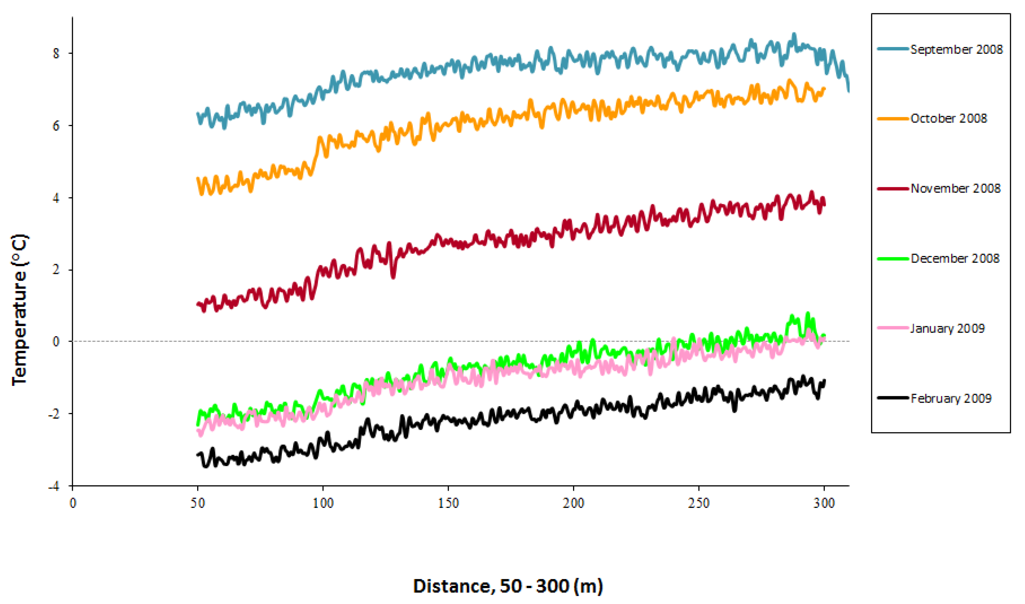
According to the initial measurement period in 2008–2009, the cooling of the sediment took place until February 2009, when the lowest temperatures were measured. Sediment temperatures were very close together in December and January. The sediment temperatures for a six-month period in 2008–2009 are shown in Figure 2 (Huusko, A; Martinkauppi, I. Geological Survey of Finland. Personal communication, 2009). This was the first season in which the houses were heated using the low energy network. The sediment temperatures were presented from a distance of 50 to 300 m from the shore. This distance was chosen because 0–50 m is relatively close to the shore and, therefore, flora (reeds, etc.) might affect the temperatures.
The mean air temperature in Ostrobothnia in the year 2008 was over 5.0 °C and in the year 2009, it was 4.0–5.0 °C [22]. The monthly mean air temperature in Vaasa is shown in Table 1 (Pirinen, P. Finnish Meteorological Institute. Personal Communication, 2017). The heating season began in October, which can be observed as a decrease in sediment temperatures in November 2008. Further, the mean air temperatures were already dropping when the winter season arrived. A high and significant correlation has been observed between the air temperature and the temperature of sediment after one or two months [21]. The value of the maximum sediment temperature per month (Table 1) was calculated as an average of temperatures at a distance of 280–300 m from the shore (Huusko, A; Martinkauppi, I. Geological Survey of Finland. Personal communication, 2009).
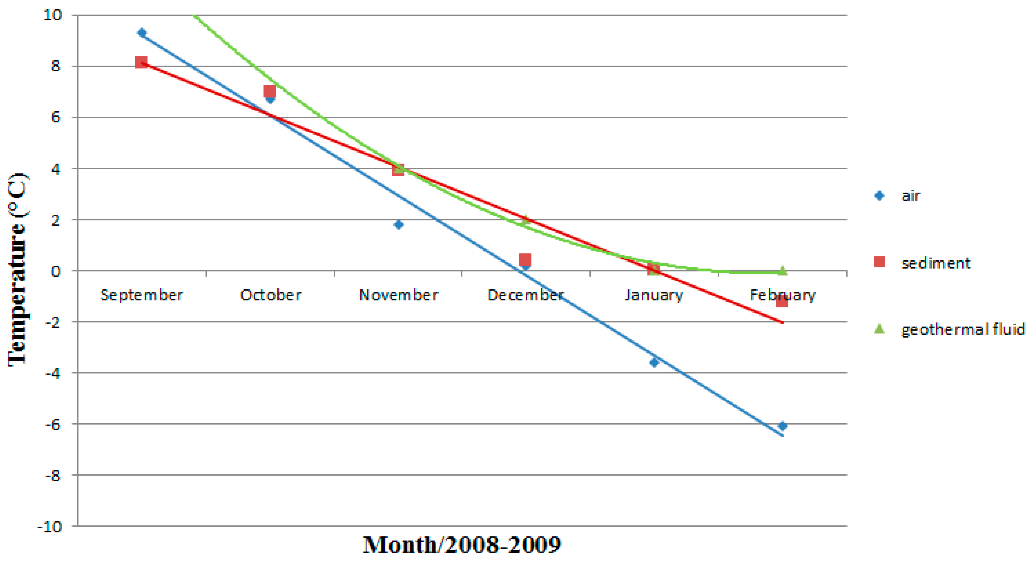
The temperatures of the geothermal fluid were measured for the period November 2008 to February 2009 in one house connected to the low energy network. The relationship between the temperatures of the air, sediment and geothermal fluid from September 2008 to February 2009 are shown in Figure 3. In December, the geothermal fluid was measured as slightly warmer than the sediment, which can be explained by the different measurement locations.
The loading of sediment heat is shown in Figure 4. The temperatures of the sediment increased between March and August up to 11–12 °C. By May, the ambient air had warmed up and the snow and ice had melted. The water was becoming warmer and the heat in the sediment layer was also increasing. Another great difference in sediment temperatures occurred between June and July. This indicates the end of the house-heating season. The heat loading in the sediment layer starts from the shore and goes to the end of the pipe, which can be observed as a constant curve without any slope in July and August.
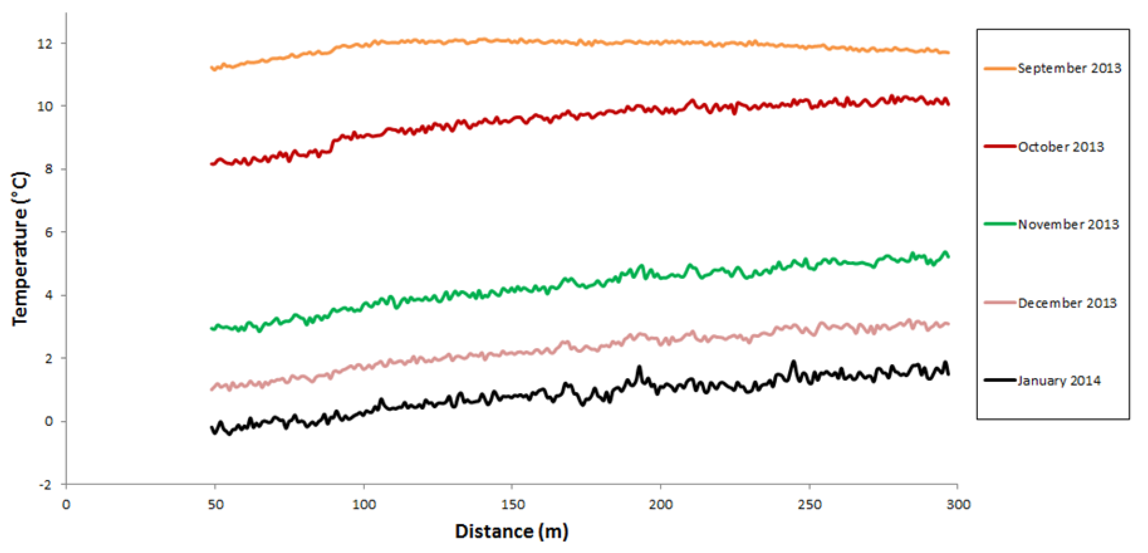
In the follow-up study of 2013–2014, the sediment temperature cooled down until January 2014 (Figure 5). The heating of houses began in October, which can be seen in the great sediment temperature difference between October and November.
The mean air temperature in Ostrobothnia, Finland in 2013 was 5–6 °C [22]. The monthly mean air temperatures in Vaasa for a five-month period in 2013–2014 are presented in Table 2 (Pirinen, P. Finnish Meteorological Institute. Personal Communication, 2017). During the measurement period of 2013–2014, it can be noticed that, on average, the sediment temperatures were higher than the air temperatures in every month except September, when they were almost equal.
The relationship between the temperatures of the air, sediment and geothermal fluid in the period September 2013 to January 2014 are shown in Figure 6. The temperatures of the geothermal fluid were cooler than the sediment temperatures for the whole measurement period of 2013–2014.
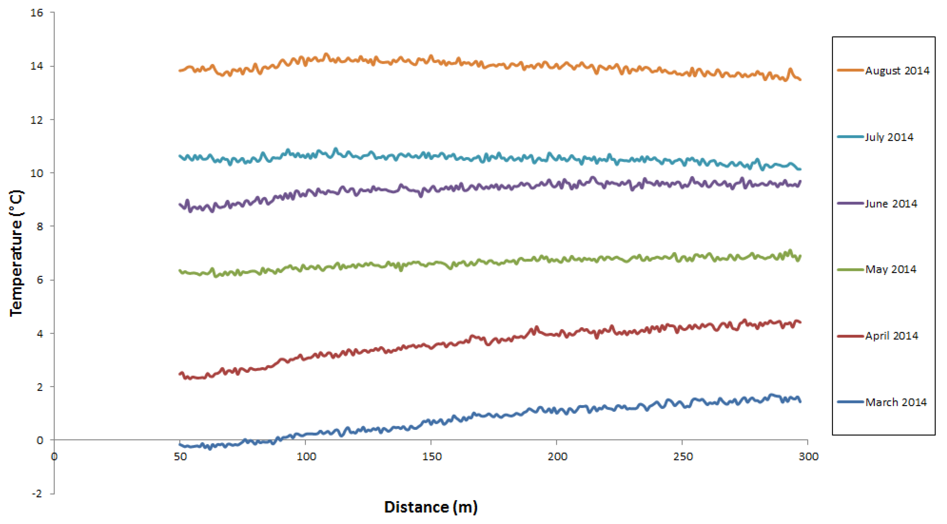
The warming of the sediment layer from spring to late summer 2014 is shown in Figure 7. The temperatures of the sediment were increasing by up to 14 °C from March to August. The greatest difference in sediment temperatures is between April and May. The heat loading in the sediment layer takes place along the whole area from the shore to the distance of 300 m, which can be observed as a constant curve without any slope in July and August. The difference in temperatures in July and August is about 3.5 °C. The effect of the Sun is obvious.
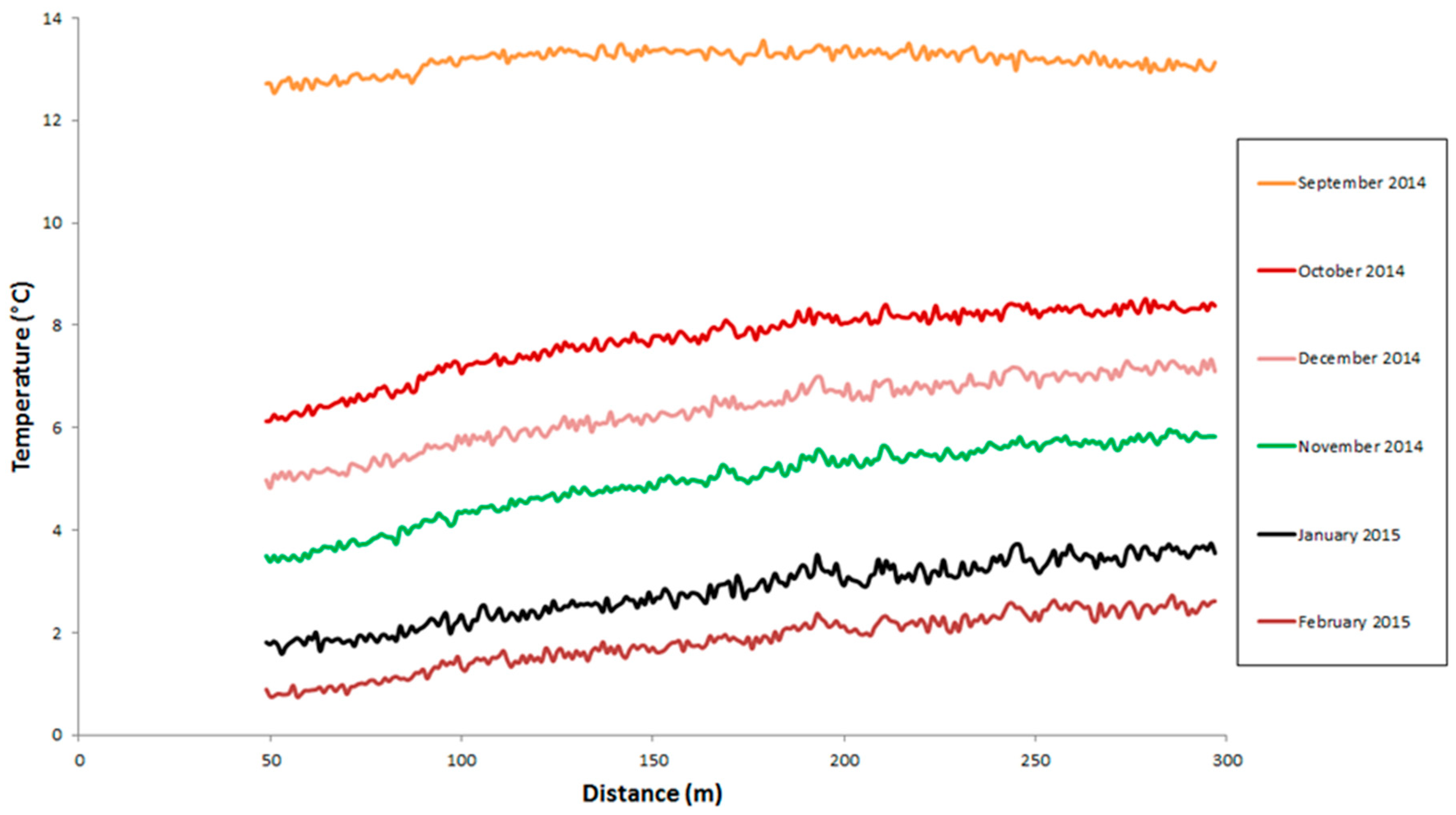
In the final follow-up study, 2014–2015, the sediment was cooling down until February 2015 (Figure 8). The great gap between the temperatures measured in September and October is due to the start of the house-heating season. Exceptionally, the sediment in December was warmer than in November. The autumn of 2014 was unusual in terms of sea water and air temperatures [22]. Energy consumption was minor in November and the heat was gathering close to the collection pipe.
The mean air temperature in Ostrobothnia, Finland in 2014 was 6.1 °C and in 2015 it was 6.4 °C (Pirinen, P. Finnish Meteorological Institute. Personal Communication, 2017). The monthly mean air temperatures in Vaasa in a six-month period in 2014–2015 are presented in Table 3. In the measurement period 2014–2015, it can be seen that, on average, in every month, the sediment temperatures were higher than the air temperatures. Further, the sediment temperatures were higher than the geothermal fluid temperatures for the whole period.
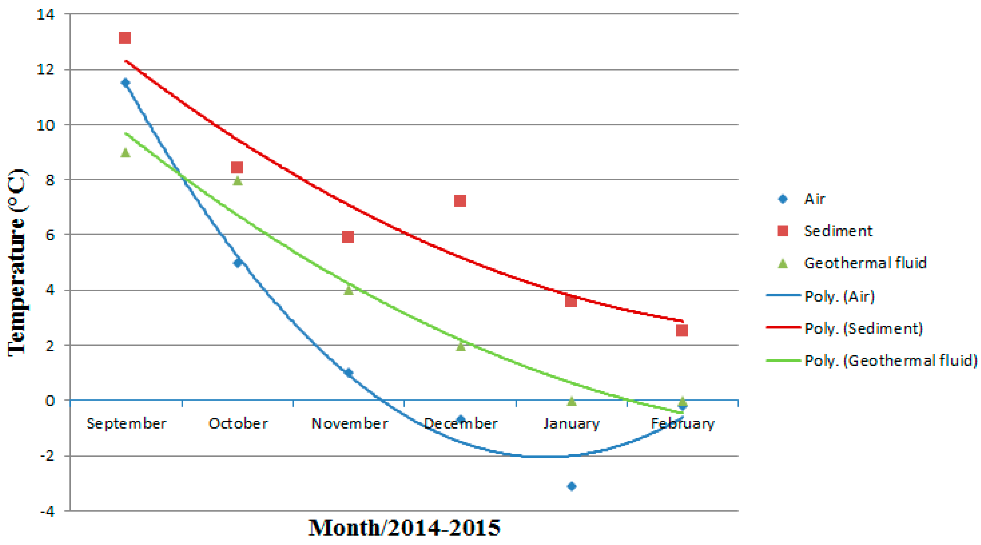
The relationship between the temperatures of the air, sediment and geothermal fluid in the period September 2014 to February 2015 are shown in Figure 9. The sediment was warmer than the air during the whole period. The geothermal fluid temperatures were cooler than the sediment temperatures for the whole measurement period of 2014–2015, as expected.
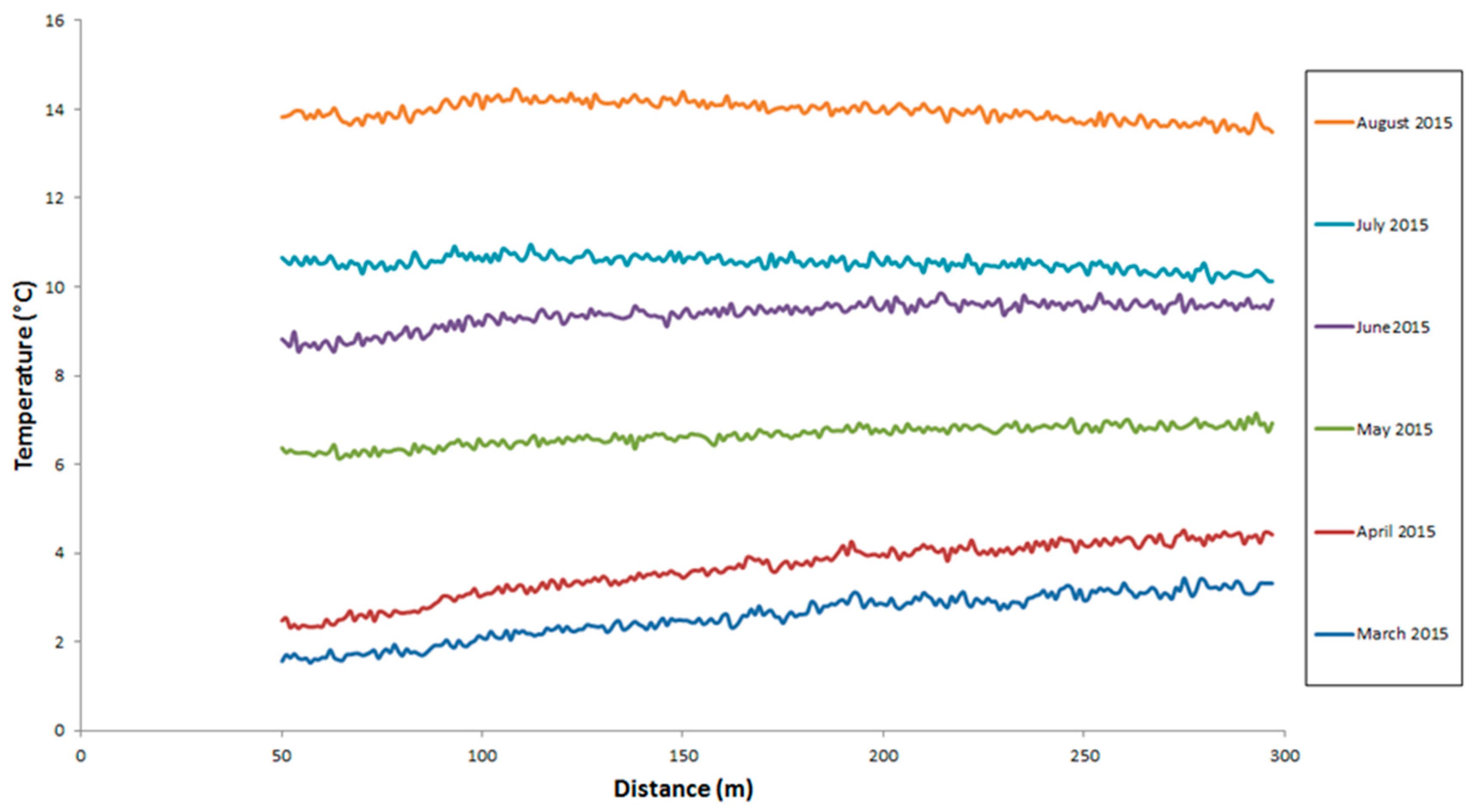
The warming of the sediment layer from spring to late summer 2015 is shown in Figure 10. The temperatures of sediment were increasing from March to August, by up to 12 °C. The greatest difference in the sediment temperatures was between April and May and the sediment had clearly warmed up by July.
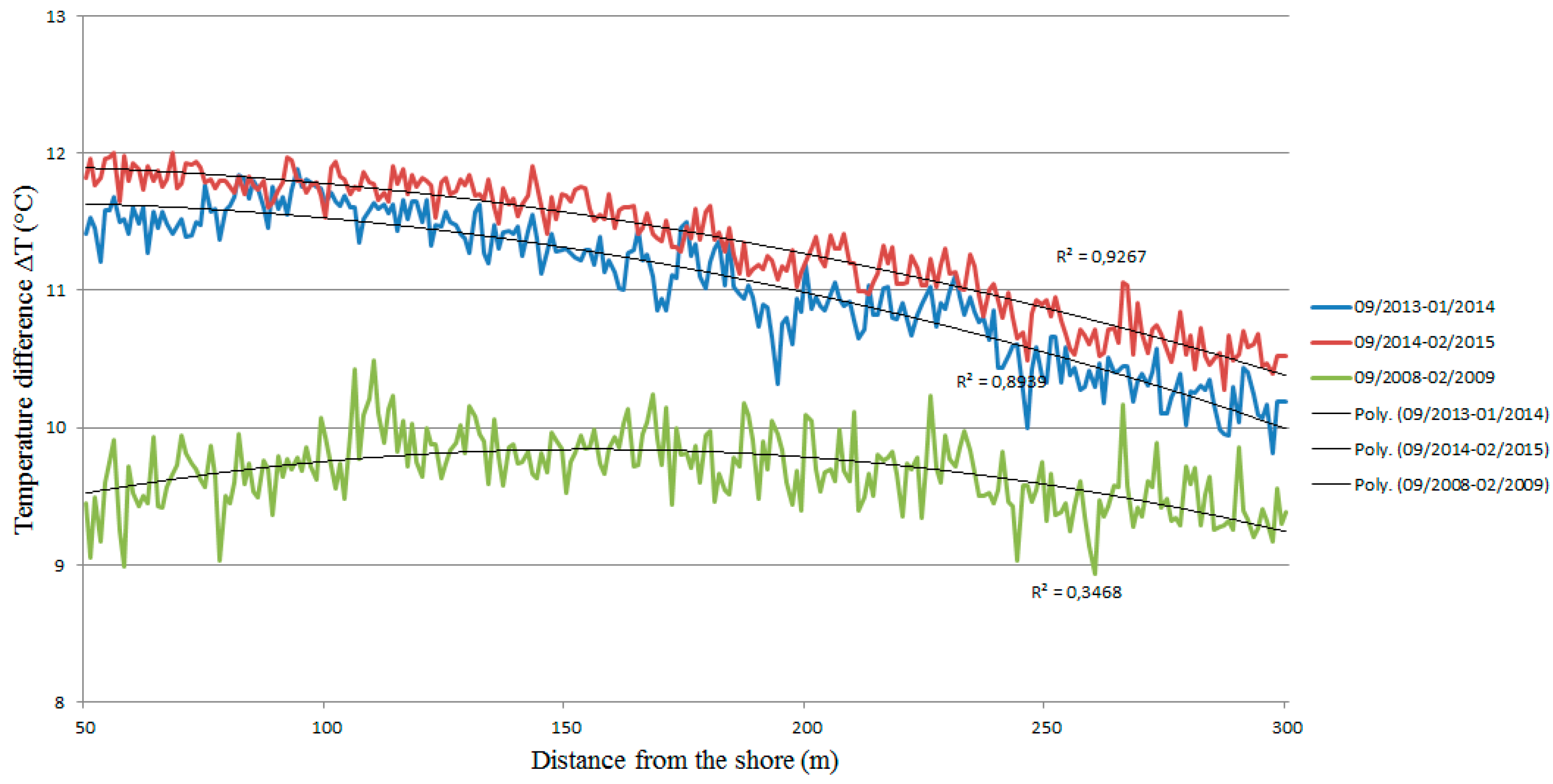
In 2008–2009, the average difference between the sediment temperature in September (the month with the highest temperature value) and February (the month with the coldest sediment temperature) was 9.7 °C. In 2013–2014, the average difference between the sediment temperature in September and that of the month with the lowest sediment temperature, i.e., January, was 11.1 °C. In 2014–2015, the difference between the temperature in September and the lowest temperature values in February was 11.2 °C. Thus, the absolute decrease in temperature was essentially the same in both periods (Figure 11).
In the years 2013–2014 and 2014–2015 the difference in temperatures was higher nearer to the shore and decreased smoothly, being around 1.5 °C lower at the distance of 300 m than at the distance of 50 m from the shore.
5. Discussion
Different models of interaction between water and sediment has been studied e.g., in North-Western Russia and Germany, [2] and in United States [10,23]. The measured data for all the periods—2008–2009, 2013–2014 and 2014–2015—show the cooling of sediment during the autumn and winter seasons. The difference in sediment temperatures between a month with the highest temperature value and a month with the lowest temperature value in each period varied from 9.7 to 11.2 °C. The level of the temperatures was about 4 °C lower in the early stage of the new low energy network (2008–2009) than it was five years later. In the first measurement period, 2008–2009, measurements were taken with a device that was different to that used in the follow-up measurement period of 2013–2015. It is also true that because of heating and the drying of the constructions, the houses needed more energy during the first heating season than they did in later years. This has had a decreasing influence on the temperatures of the sediment.
There is a roughly 2 °C difference between the temperatures measured near the shore and those measured at a distance of 300 m from the shore. This difference may reflect the depth of the water layer over the sediment. The farther from the shore the measurement is taken, the thicker the water layer and the warmer the sediment. Accurate data about the depth of the water layer are not available for the Suvilahti area. On the other hand, the position of the cable is estimated to be 3–4 m under the seabed but the exact position of the cable at the different distances from the shore cannot be measured.
In the measurement period 2008–2009, the heat carrier fluid temperature was higher than the highest sediment temperature each month in that period. This is explained by the accuracy of the Ouman fluid temperature meter, which was ±1 degree. The result is intelligible if the limit of error is taken into account. The other factor that may have had an effect on the comparability of the fluid and sediment temperatures is that the measurements of the heat carrier fluid were made in the engineering and utility service room inside a house, whereas the sediment temperature measurements were taken next to the collection well on the shore. It may also be possible that the surroundings of the collection pipe in the seabed sediment were frozen and that ice cover may have acted as an insulator for the heat carrier fluid.
The validity of the sediment temperature data is somewhat questionable because of the location of the temperature measurement cable, i.e., connected to the side of the operating heat collection pipe that contains the heat carrier fluid. On the other hand, the influence of the fluid can be expected to be quite small. In future studies, to gain more accurate sediment temperatures, it would be good to attach the temperature measurement cable to bare sediment in the same location and to compare those temperatures with the current results.
The possible flow of groundwater should be known when estimating the heat capacity of a particular area of the sediment. These data are missing for Suvilahti.
Ice and snow cover have an effect on the temperatures of water, which, according to Birge et al. [6] interacts with the sediment. There are no data available about the thickness of the ice or the depth of snow cover in Suvilahti. The stationary stage of sediment temperatures can be observed in a particular section of every study period and this reflects the impact of ice and snow cover. The heat transfer occurs farther from the pipeline and a stationary stage prevails close to the pipeline.
6. Conclusions
These follow-up sediment temperature measurements show that sediment has reloaded perfectly every year. Despite the usage of the energy, the temperature rate of the sediment did not essentially decrease during the five-year period in the Vaasa Housing Fair area. The start of the heating season can be clearly observed.
Consideration of the between-month difference in sediment temperatures for the month with the highest temperature and the month with the lowest temperature value for all measurement periods shows that the usage of the low energy network has not permanently changed temperatures in the sediment. The temperatures vary annually and the influence of the radiant energy of the Sun can be noted. The accumulation of heat can be seen in the sediment temperatures in autumn as the highest values of the year.
There is a drop of several degrees in the temperatures of October The first heating month harvests the energy from areas close to the heat collection pipe. The sea has yet no covering of ice. The air temperature has an influence on the water and, due to heat conduction, also on the sediment temperatures. All this appears as a notable decrease in the sediment temperature in November and continues until the stationary stage has been achieved in February–March 2009, January–March 2014 and January–March 2015.
This research indicates that the sediment heat is a potential energy source. In future development of these systems the depth of the pipeline should be known and kept in at least 3 m downwards from the sea bottom.
Acknowledgments
We would like to express our thanks to Juhani Luopajärvi (heat carrier fluid measurements) and the Geological Survey of Finland in Kokkola. This work was supported by the City of Vaasa and the University of Vaasa.
Author Contributions
Anne Mäkiranta and Erkki Hiltunen conceived and designed the experiments; Anne Mäkiranta performed the experiments, analyzed the data and wrote the paper; Birgitta Martinkauppi contributed to the theory; Mauri Lieskoski contributed to the materials.
Conflicts of Interest
The authors declare no conflict of interest. The founding sponsors had no role in the design of the study; in the collection, analyses, or interpretation of data; in the writing of the manuscript and in the decision to publish the results.
References
- Likens, G.E.; Johnson, N.M. Measurement and analysis of the annual heat budget for the sediments in two Wisconsin lakes. Limnol. Oceanogr. 1969, 14, 115–135. [Google Scholar] [CrossRef]
- Golosov, S.; Kirillin, G. A parameterized model of heat storage by lake sediments. Environ. Model. Softw. 2010, 25, 793–801. [Google Scholar] [CrossRef]
- Finnish Meteorological Institute. Available online: http://ilmatieteenlaitos.fi/tilastoja-vuodesta-1961 (accessed on 12 October 2017). (In Finnish).
- Mäkiranta, A.; Martinkauppi, J.B.; Hiltunen, E. Seabed sediment—A natural seasonal heat storage feasibility study. Agron. Res. 2017, 15, 1101–1106. [Google Scholar]
- Birge, E.A.; Juday, C.; March, H.W. The temperature of the bottom deposits of Lake Mendota; a chapter in the heat exchanges of the lake. Trans. Wis. Acad. Sci. 1927, XXIII, 187–231. [Google Scholar]
- Smith, N.P. Observations and simulations of water-sediment heat exchange in a shallow coastal lagoon. Estuaries 2002, 25, 483–487. [Google Scholar] [CrossRef]
- Gu, R.; Stefan, H.G. Year-round temperature simulation of cold climate lakes. Cold Reg. Sci. Technol. 1990, 18, 147–160. [Google Scholar] [CrossRef]
- Hondzo, M.; Ellis, C.; Stefan, H. Vertical diffusion in small stratified lake: Data and error analysis. J. Hydraul. Eng. 1991, 117, 1352–1369. [Google Scholar] [CrossRef]
- Welch, H.E.; Bergmann, M.A. Water circulation in small arctic lakes in winter. Can. J. Fish. Aquat. Sci. 1985, 42, 506–520. [Google Scholar] [CrossRef]
- Tsay, T.; Ruggaber, G.J.; Effler, S.W.; Driscoll, C.T. Thermal stratification modeling of lakes with sediment heat flux. J. Hydraul. Eng. 1992, 118, 407–419. [Google Scholar] [CrossRef]
- Bengtsson, L. Mixing in ice-covered lakes. Hydrobiologia 1996, 322, 91–97. [Google Scholar] [CrossRef]
- Fang, X.; Stefan, H.G. Dynamics of heat exchange between sediment and water in a lake. Water Resour. Res. 1996, 32, 1719–1727. [Google Scholar] [CrossRef]
- Brewer, M.C. The thermal regime of an arctic lake. Am. Geophys. Union Trans. 1958, 39, 278–284. [Google Scholar] [CrossRef]
- Allen, A.; Dejan, M.; Sikora, P. Shallow gravel aquifers and the urban ‘heat island’ effect: A source of low enthalpy geothermal energy. Geothermics 2003, 32, 569–578. [Google Scholar] [CrossRef]
- Zhu, K.; Blum, P.; Ferguson, G.; Balke, K.; Bayer, P. The geothermal potential of urban heat islands. Environ. Res. Lett. 2010, 5, 1–6. [Google Scholar] [CrossRef]
- Suomi, J. Characteristics of Urban Heat Island (UHI) in a High-Latitude Coastal City—A Case Study of Turku. SW Finland. Ph.D. Thesis, Department of Geography and Geology, University of Turku, Turku, Finland, 2014; 70p. Available online: http://urn.fi/URN:ISBN:978-951-29-5912-9 (accessed on 21 November 2017).
- Li, C.; Shang, J.; Cao, Y. Discussion on energy-saving taking urban heat island effect into account. In Proceedings of the IEEE International Conference on Power System Technology (POWERCON), Hangzhou, China, 24–28 October 2010; pp. 1–3. [Google Scholar]
- Santamouris, M. Solar Thermal Technologies for Buildings—The State of the Art; Cromwell Press: Trowbridge, UK, 2003; ISBN 1-902916-47-6. [Google Scholar]
- Hiltunen, E.; Martinkauppi, B.; Zhu, L.; Mäkiranta, A.; Lieskoski, M.; Rinta-Luoma, J. Renewable, carbon-free heat production from urban and rural water areas. J. Clean. Prod. 2017, 153, 397–404. [Google Scholar] [CrossRef]
- Hiltunen, E.; Martinkauppi, J.B.; Mäkiranta, A.; Rinta-Luoma, J.; Syrjälä, T. Seasonal temperature variation in heat collection liquid used in renewable, carbon-free heat production from urban and rural water areas. Agron. Res. 2015, 13, 485–493. [Google Scholar]
- Mäkiranta, A.; Martinkauppi, J.B.; Hiltunen, E. Correlation between temperatures of air, heat carrier liquid and seabed sediment in renewable low energy network. Agron. Res. 2016, 14, 1191–1199. [Google Scholar]
- Finnish Meteorological Institute. Available online: http://ilmatieteenlaitos.fi/jaatalvi-2014-2015 (accessed on 11 December 2017). (In Finnish).
- Fang, X.; Stefan, H.G. Temperature variability in lake sediments. Water Resour. Res. 1998, 34, 717–729. [Google Scholar] [CrossRef]
Figure 1.
(a) Profile of the heat collector pipe and the location of an optical cable; (b) The assembling of heat collection pipes.
Figure 1.
(a) Profile of the heat collector pipe and the location of an optical cable; (b) The assembling of heat collection pipes.

Figure 2.
Seabed sediment temperatures measured from September 2008 to February 2009 in Liito-oravankatu.
Figure 2.
Seabed sediment temperatures measured from September 2008 to February 2009 in Liito-oravankatu.

Figure 3.
The relationship between the air, sediment and geothermal fluid temperatures in the low energy network of Suvilahti, Vaasa, 2008–2009. The lines are drawn to visualize and approximate relationship between measurements points.
Figure 3.
The relationship between the air, sediment and geothermal fluid temperatures in the low energy network of Suvilahti, Vaasa, 2008–2009. The lines are drawn to visualize and approximate relationship between measurements points.

Figure 4.
Seabed sediment temperatures measured from March 2009 to August 2009 in Liito-oravankatu. The Sun is obviously loading the heat to the seabed sediment.
Figure 4.
Seabed sediment temperatures measured from March 2009 to August 2009 in Liito-oravankatu. The Sun is obviously loading the heat to the seabed sediment.

Figure 5.
Seabed sediment temperatures measured from September 2013 to January 2014 in Liito-oravankatu.
Figure 5.
Seabed sediment temperatures measured from September 2013 to January 2014 in Liito-oravankatu.

Figure 6.
Temperatures of air, sediment and geothermal fluid in measurement period 2013–2014.

Figure 7.
Seabed sediment temperatures measured from March 2014 to August 2014 in Liito-oravankatu. Temperatures increase after the winter months.
Figure 7.
Seabed sediment temperatures measured from March 2014 to August 2014 in Liito-oravankatu. Temperatures increase after the winter months.

Figure 8.
Seabed sediment temperatures measured from September 2014 to February 2015 in Liito-oravankatu.
Figure 8.
Seabed sediment temperatures measured from September 2014 to February 2015 in Liito-oravankatu.

Figure 9.
Temperatures of the air, sediment and geothermal fluid in the measurement period 2014–2015.
Figure 9.
Temperatures of the air, sediment and geothermal fluid in the measurement period 2014–2015.

Figure 10.
Seabed sediment temperatures measured from March 2015 to August 2015 in Liito-oravankatu. Heat loading is observed as increased temperatures in the sediment layer.
Figure 10.
Seabed sediment temperatures measured from March 2015 to August 2015 in Liito-oravankatu. Heat loading is observed as increased temperatures in the sediment layer.

Figure 11.
The between-month difference in sediment temperatures for the months with the highest and the lowest temperature values in the periods 2008–2009, 2013-2014 and 2014-2015. The polynomials of second degree are drawn as trend lines.
Figure 11.
The between-month difference in sediment temperatures for the months with the highest and the lowest temperature values in the periods 2008–2009, 2013-2014 and 2014-2015. The polynomials of second degree are drawn as trend lines.


Table 1.
The monthly mean air temperatures (tka_air) and the monthly maximum sediment temperatures (tmax_sed) and the geothermal fluid temperatures (tka_fluid) in Vaasa during the measurement period in 2008–2009.
Table 1.
The monthly mean air temperatures (tka_air) and the monthly maximum sediment temperatures (tmax_sed) and the geothermal fluid temperatures (tka_fluid) in Vaasa during the measurement period in 2008–2009.
| Year | Month | tka_air [°C] | tmax_sed [°C] | tka_fluid [°C] |
|---|---|---|---|---|
| Air | Sediment | Geothermal Fluid | ||
| 2008 | September | 9.3 | 8.1 | - |
| October | 6.7 | 7.0 | - | |
| November | 1.8 | 3.9 | 4.0 | |
| December | 0.2 | 0.4 | 2.0 | |
| 2009 | January | −3.6 | 0 | 0.0 |
| February | −6.1 | −1.2 | 0.0 |
Table 2.
The monthly mean air temperature (tka_air), the maximum sediment temperatures (tmax_sed) and the geothermal fluid temperatures (tka_fluid) in Vaasa in the measurement period 2013–2014.
Table 2.
The monthly mean air temperature (tka_air), the maximum sediment temperatures (tmax_sed) and the geothermal fluid temperatures (tka_fluid) in Vaasa in the measurement period 2013–2014.
| Year | Month | tka_air [°C] | tmax_sed [°C] | tka_fluid [°C] |
|---|---|---|---|---|
| Air | Sediment | Geothermal Fluid | ||
| 2013 | September | 11.9 | 11.7 | 10.0 |
| October | 6.3 | 10.2 | 7.0 | |
| November | 2.6 | 5.2 | 5.0 | |
| December | 0.8 | 3.1 | 2.0 | |
| 2014 | January | −8.0 | 1.6 | 0.0 |
Table 3.
The monthly mean air temperature (tka_air), the maximum sediment temperatures (tmax_sed) and the geothermal fluid temperatures (tka_fluid) in Vaasa in the measurement period 2014–2015.
Table 3.
The monthly mean air temperature (tka_air), the maximum sediment temperatures (tmax_sed) and the geothermal fluid temperatures (tka_fluid) in Vaasa in the measurement period 2014–2015.
| Year | Month | tka_air [°C] | tmax_sed [°C] | tka_fluid [°C] |
|---|---|---|---|---|
| Air | Sediment | Geothermal Fluid | ||
| 2014 | September | 11.5 | 13.1 | 9.0 |
| October | 5.0 | 8.4 | 8.0 | |
| November | 1.0 | 5.9 | 4.0 | |
| December | −0.7 | 7.2 | 2.0 | |
| 2015 | January | −3.1 | 3.6 | 0.0 |
| February | −0.2 | 2.5 | 0.0 |
© 2018 by the authors. Licensee MDPI, Basel, Switzerland. This article is an open access article distributed under the terms and conditions of the Creative Commons Attribution (CC BY) license (http://creativecommons.org/licenses/by/4.0/).
Share and Cite
MDPI and ACS Style
Mäkiranta, A.; Martinkauppi, B.; Hiltunen, E.; Lieskoski, M. Seabed Sediment as an Annually Renewable Heat Source. Appl. Sci. 2018, 8, 290. https://0-doi-org.brum.beds.ac.uk/10.3390/app8020290
AMA Style
Mäkiranta A, Martinkauppi B, Hiltunen E, Lieskoski M. Seabed Sediment as an Annually Renewable Heat Source. Applied Sciences. 2018; 8(2):290. https://0-doi-org.brum.beds.ac.uk/10.3390/app8020290
Chicago/Turabian StyleMäkiranta, Anne, Birgitta Martinkauppi, Erkki Hiltunen, and Mauri Lieskoski. 2018. "Seabed Sediment as an Annually Renewable Heat Source" Applied Sciences 8, no. 2: 290. https://0-doi-org.brum.beds.ac.uk/10.3390/app8020290
Note that from the first issue of 2016, this journal uses article numbers instead of page numbers. See further details here.