An Evolutionary-Based MPPT Algorithm for Photovoltaic Systems under Dynamic Partial Shading


Department of Energy, Politecnico di Milano, via La Masa 34, 20156 Milano, Italy
*
Author to whom correspondence should be addressed.
Appl. Sci. 2018, 8(4), 558; https://0-doi-org.brum.beds.ac.uk/10.3390/app8040558
Submission received: 8 March 2018
/
Revised: 28 March 2018
/
Accepted: 29 March 2018
/
Published: 4 April 2018
(This article belongs to the Special Issue Computational Intelligence in Photovoltaic Systems)
Abstract
:The increase of renewable energy usage in the last two decades, in particular photovoltaic (PV) systems, has opened up different solar plant configurations that need to operate and properly perform in terms of efficient power transfer with respect to all of the involved components, such as inverters, grid interface, storage, and other electrical loads. In such applications, the power characteristics of the plant modules all together represent the main components that are responsible for power extraction, depending on both external and internal factors. Conventional maximum power point tracking techniques may not have a proper conversion efficiency under particular external dynamic conditions. This paper proposes an evolutionary-based maximum power point tracking algorithm suitable to operate under dynamic partial shading conditions and compares its performance with classical maximum power point tracking methods in order to evaluate their conversion efficiency in partial shading scenarios with relevant and dynamic changes in the environmental conditions. Simulations taking into account the different dynamic shading conditions were carried out to prove the effectiveness and limitations of the proposed approach with respect to classical algorithms.
1. Introduction
Solar energy is one of most reliable, cleanest, and easy to harvest energy sources among all renewables. Solar energy can be converted into other forms of energy, mostly electricity and heat. Solar cells convert sunlight directly into electricity, while concentrating solar power systems use mirrors to concentrate the energy from the sun to heat a working fluid that drives traditional steam turbines connected to an electrical power generator. Over the last two decades, worldwide solar photovoltaic (PV) installations have exponentially grown and their cost has significantly reduced due to the improvements in technology and the economies of scale. Besides direct economic and environmental advantages, the use of solar energy produces other indirect environmental and social benefits, such as the stabilization of degraded land, the increasing of energy independence, new job opportunities, acceleration of remote rural areas electrification, and improved quality of life in developing countries [1]. The environmental issues related to the installation of solar power facilities have been comprehensively addressed in [2]: more than thirty environmental impacts falling in the fields of land use intensity, human health and wellbeing, plant and animal life, geo-hydrological resources, and climate change. In this context, the integration of solar energy into islanded micro-grids can play a key role both in decreasing the dependence on fossil fuels in energy intensive applications, for example in the desalination of plants [3], and to speed up access to electricity in developing countries [4].
The high penetration of renewables in the power grid presents several challenges, mainly related to the uncertainty in generation output due to weather fluctuations. In recent years, several Computational Intelligence (CI) techniques have been developed for renewable energies [5], with the aim of helping grid operators to better manage the electric balance between power demand and supply. In particular, the efficiency of a whole PV system depends on many factors at the same time: the efficiency of each single PV module [6,7], mismatch losses in the PV generator [8,9], losses in the wiring, switches, transformers and power converters, and the extraction efficiency of the Maximum Power Point Tracking (MPPT) algorithm. Moreover, the efficiency of the hardware components is neither easily or cheaply improved, but the improvement of the MPPT with new control algorithms allows for increasing power generation performance. In this context, CI techniques can be successfully employed to tackle various problems in system optimization and power extraction strategy [10]. In this light, the Particle Swarm Optimization (PSO) is a well-known evolutionary algorithm based on a model of group interaction between independent agents (particles) that uses social behavior (or swarm knowledge) in order to find a global maximum or minimum of a specific fitness function [11]. This computational technique adopts a biological-like approach, and takes its rationale from the emulation of social behaviors such as those related to bird flocking and fish schooling. The PSO algorithm explores the problem domain with moving particles represented by a set of coordinates in the N-dimensional solution space, which represents a specific problem solution corresponding to a particular value of the objective function.
This work proposes a novel MPPT algorithm based on the PSO evolutionary approach and compares the results with traditional MPPT methods, previously tested by the authors [12], with the aim of increasing the overall conversion efficiency in particular conditions characterized by relevant changes and high dynamism with an affordable computational burden. This optimization of solar power extraction requires operating the photovoltaic generator at its maximum efficiency and can naturally benefit evolutionary computation. Numerous research studies on MPPT for solar PV systems have been proposed in last few decades and the methods developed so far can be broadly classified into conventional versus soft computing techniques [13].
Conventional MPPT algorithms are based on search algorithms designed to find the maximum output in different external conditions [14], but only under uniform irradiation. These methods generally fail when partial shading occurs on the PV generator, showing poor convergence, slow tracking speed, and often high steady state oscillations [15,16]. Among the conventional MPPT methods, the most popular are Perturb and Observe (P&O) [17] and Incremental Conductance (IC) [18].
In order to overcome the drawbacks of a specific conventional MPPT technique and to gain better performance, various methods are combined to set up MPPT hybrid algorithms [19,20]. Soft computing and evolutionary algorithms can offer some advantages, such as their ability to handle non linearity, a wide exploration in search space, and coherent skill to reach global optimal regions [15]. Moreover, they can be combined with conventional MPPT techniques [21,22] in order to further improve their efficiency.
In literature, other comparative studies can be found among different MPPT algorithms on PV modules under dynamic shading conditions [23,24]. Since partial shading on PV modules may result in power curves with multiple peaks and multiple local minima and maxima [25], the main advantage of using evolutionary computation techniques results in their acting as an effective global optimizer. In this context, the PSO-based MPPT algorithm here proposed appears to be a good tradeoff between simplicity in implementation and accuracy in the tracking of the Global Maximum Power Point (GMPP). This work aims also to compare this novel algorithm based on a bio-inspired approach with traditional MPPT methods in order to evaluate efficiency under partial and dynamic shading conditions.
The paper is structured as follows: Section 2 describes critical issues of MPPT algorithms under partial shading conditions and describes, step by step, the proposed MPPT algorithm based on the PSO evolutionary approach. Section 3 reports the simulated test case scenario with related applied shading conditions. Section 4 shows the numerical results and the preliminary experimental tests of the proposed algorithm in comparison with other classical MPPT algorithms with respect to different shading objects and various dynamics. Section 5 draws conclusions based on the results.
2. Evolutionary-Based MPPT Algorithm for PV System Power Extraction
2.1. MPPTs and PV System Issues Under Dynamic Partial Shading
PV generators are highly dependent on environmental conditions such as solar irradiance, temperature, and particular shading conditions. The natural variation of such environmental parameters combined with the nonlinear characteristics of the solar cells make power extraction optimization a critical task. To obtain the maximum conversion efficiency, the PV generator must operate at the higher point of its power-voltage curve, also called the Maximum Power Point (MPP). This control is known as the Maximum Power Point Tracking, and it is the typical operating condition of PV generators both in grid-connected and off-grid PV systems. Only in very special cases, the PV generator is regulated at a lower power than the MPP with the algorithm of Regulated Power Point Tracking (RPPT), as in the case of islanded hybrid micro-grids where the power production exceeds the load demand and storage systems are not available [4]. Various MPPT techniques have been developed over the last years that follow both direct and indirect approaches.
When particular shading conditions occur on a PV generator, one or more bypass diodes can be forward biased to prevent localized power dissipation at the shaded cells. The bypass diodes forward or reverse bias state under partial shading depends on the PV generator output voltage, resulting in modified P-V curves with multiple local maxima. Thus, the MPPT algorithm running in the control unit must be adapted or modified when designing an algorithm suitable to operate in the case of partial shading and rapidly changing environmental conditions.
Traditional Perturb and Observe methods (P&Os) simply compare the actual PV generator voltage and output power with respect to the previous ones, adapting the operating points accordingly to reach the MPP condition. However, when rapid environmental changes occur, even the most sophisticated variant of P&Os may lose efficiency, since these hill climbing techniques may not always reach the GMPP and the operating point may get stuck in a local maxima.Thus, it is possible to conceive a family of PSO-based MPPT algorithms, with a variable population size, in order to better find the proper MPP. On the other hand, by increasing the number of particles, the computational time increases and the conversion efficiency decreases. Thus, in the context of PSO-based MPPT algorithms it is better to keep the population size as small as possible. Moreover, in this particular application characterized by dynamic partial shading, a time-varying fitness function has to be considered. Among all other evolutionary techniques, Particle Swarm Optimization is characterized by easy implementation. In this particular context, the exploitation feature of this algorithm can guarantee to reach the MPP without oscillations. Knowing a priori the number of potential local maxima related to the specific system and number of diodes, it is possible to implement a simple PSO-based algorithm with a relatively small number of agents, from three to five in this case, in order to explore the one-dimensional solution space. The next subsection describes in detail the implementation of the proposed PSO-based MPPT algorithm.
2.2. PSO-Based Algorithm Implementation
PSO is an evolutionary algorithm based on the modelling of group interaction between independent agents, also called particles, that share information about their respective search process in order to find a global maximum or minimum of a specific fitness function. Each particle represents a candidate solution and their movement in the search domain depends both on its own previous best position and the previous best position attained among all the particles. This behavior is mathematically expressed by two equations that define the velocity, vi, and the position, xi, of the i-th agent at the k-th step of the searching process:
where w is the inertia weight, c1 and c2 are the acceleration coefficients, r1 and r2 are random numbers between 0 and 1, pbest,i is the best position attained by the i-th particle and gbest is the best position attained among all the particles.
It was found that a basic problem in the application of the PSO for the MPPT system is in its random nature [16]. Very low values of r1 and r2 result in a very low velocity, thus a large number of iteration is required to reach the solution. On the other hand, too large changes in the velocity might cause the particles to move far from the neighborhood of the global maximum, opening up the possibility of converging to a local maximum instead of the global one. Moreover, in a partially shaded PV generator, the distance between the two consecutive peaks in the P-V curve is quite constant, about 80% of the open voltage of the string of PV cells connected in parallel with a bypass diode.
The goal of a MPPT algorithm is to maximize the PV output power by adjusting the duty cycle of the power converter dedicated to this function. The search of the global maximum using PSO is simple due to the fact that for this problem only a single dimensional search space is needed: the particles represent the duty cycle values and the PV generated power is the fitness function. The PSO-based MPPT algorithm presented in this work is based on a more deterministic structure, removing the random factors in (1). The velocity is limited to comply with the distance between the two peaks by tuning the coefficients c1 and c2. The search of the global maximum in the PSO-based MPPT algorithm is mathematically expressed by two equations that define the variation of the duty cycle, Δdi, and the duty cycle, di, corresponding to the i-th agent at the k-th step of the searching process:
where w is the inertia weight, c1 and c2 are the acceleration coefficients, dbest,i is the duty cycle corresponding to the maximum PV output power detected by the i-th particle and Dbest is the duty cycle corresponding to the maximum PV output power detected among all the particles.
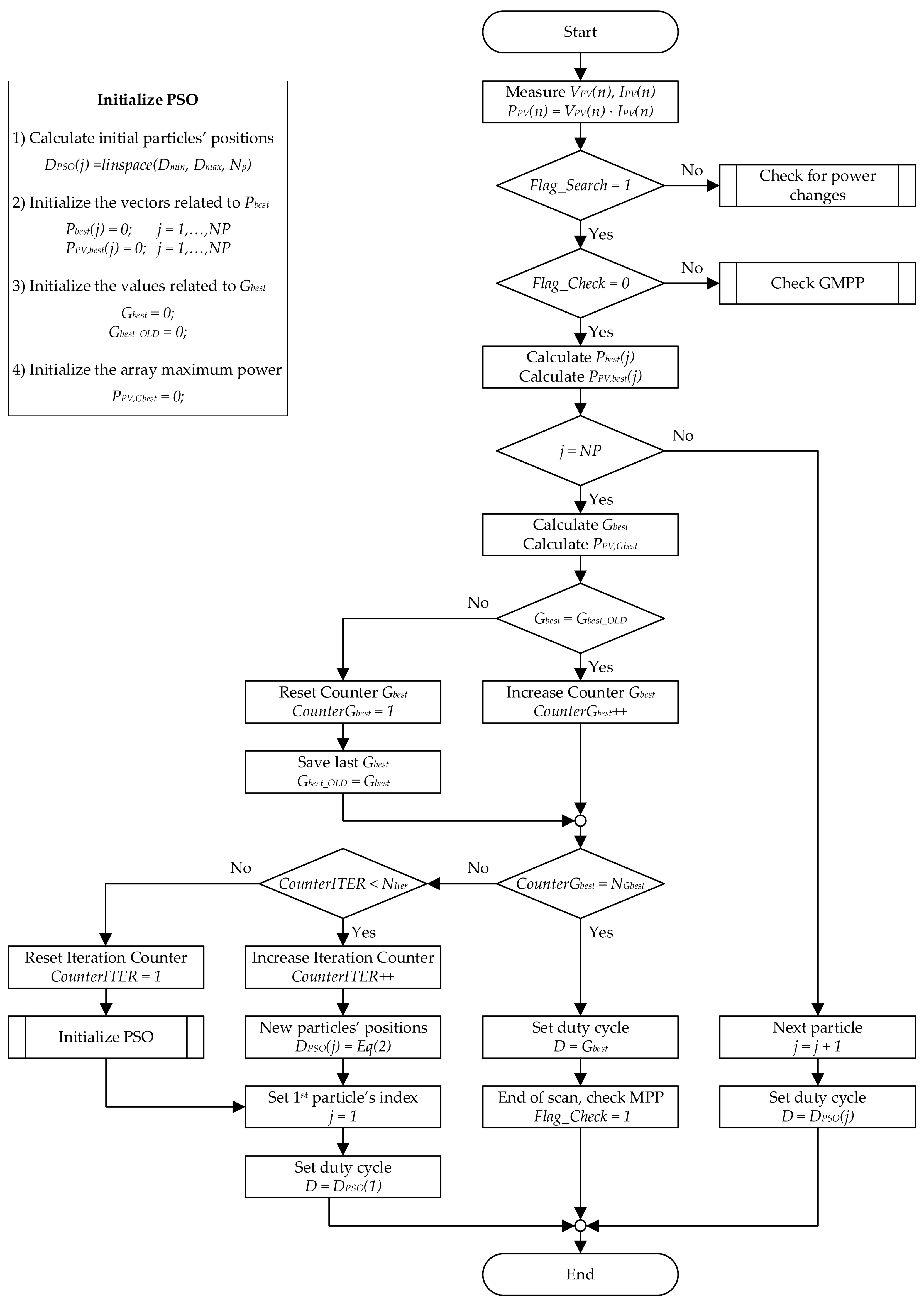
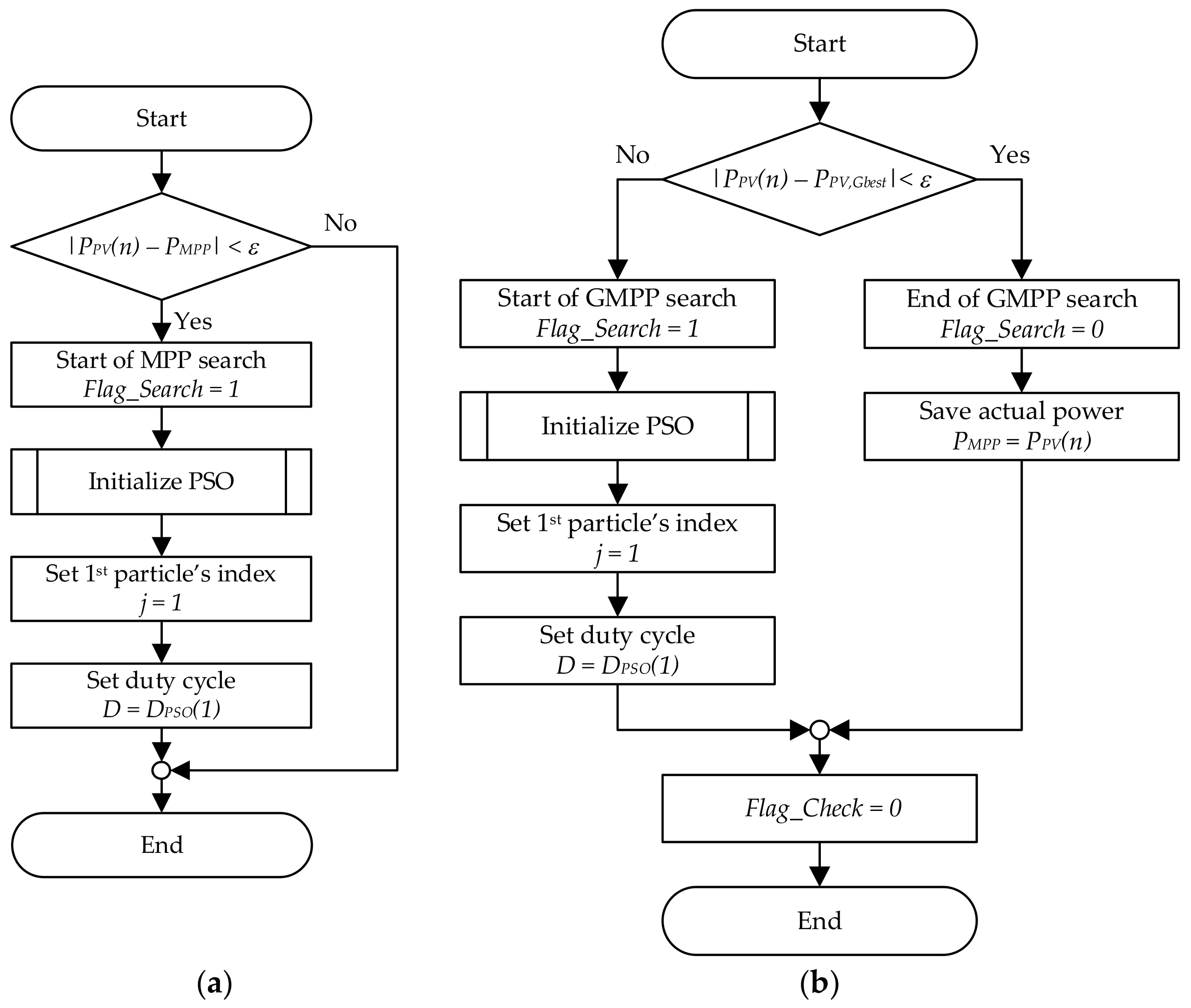
Figure 1 and Figure 2 show the flowcharts of the proposed PSO-based MPPT algorithm; they represent the program of the MPPT controller that runs at every n-th time interval.
The proposed PSO-based MPPT algorithm is organized in the following seven steps.
- Step 1:
- Activation of the MPPT algorithm. First, the MPPT controller checks whether it is necessary to activate the search for a new GMPP by comparing the actual PV power, PPV(n), with the previously recorded maximum power, PMPP. The absolute value of the difference between these powers over a threshold triggers the activation of the search for a new GMPP.
- Step 2:
- PSO Initialization. This step is the beginning of each GMPP searching process. The initial positions of the particles, namely a first solution vector of duty cycles with Np elements, are calculated: they are linearly spaced between the minimum and maximum duty cycle to cover the whole search space. All of the variables that contain information related to a previous GMPP search are reset. Then, the algorithm transmits the first duty cycle to the power converter. The change of duty cycle causes a transient of the electrical system; the new steady state condition will be evaluated at the next time interval.
- Step 3:
- Fitness Evaluation and Update Individual Best Data. The fitness value PPV(n) (actual PV output power) of the i-th particle, is calculated. Both the best individual position, dbest,i, and the best fitness, PPVbest,i, are updated in case the fitness value is greater than the best fitness. If the particle that has just been evaluated is not the last one, the algorithm transmits the next duty cycle to the power converter, whose fitness function will be evaluated at the next time interval. Otherwise, global best data will be updated and operations after each k-th iteration will be performed.
- Step 4:
- Update Global Best Data and End-of-Iteration checks. This step is the end of each k-th iteration. Both the global best position, Dbest, and the global best fitness, PPV,Gbest, are updated in case the maximum of the best fitness values of particles is greater than the global best fitness. A counter, CounterGbest, is set to 1 at every global best position update, otherwise it is incremented.
- Step 5:
- Convergence Determination and Reset Criterion. The convergence determination proposed in this work is based on the number of iterations without the update of Dbest: the convergence is reached in case a new Dbest is not found in the last NGbest iterations. Moreover, a maximum number of iterations, NIter, is allowed to reach convergence. In case the convergence is not met within the number of allowed iterations, the algorithm has to update the velocity and position of each particle and has to perform another search iteration (move to Step 6). In case the convergence is met within the number of allowed iterations, the algorithm transmits Dbest to the power converter to check the solution (move to Step 7). If the maximum number of allowed iterations is reached without convergence, the search for the GMPP has to be repeated (move to Step 2).
- Step 6:
- Update Velocity and Position of Each Particle. After all the particles are evaluated and convergence is not achieved, the velocity and the position of each particle have to be updated by using Equations (3) and (4). Then, the algorithm transmits the first duty cycles to the power converter. At the next time interval, the algorithm will move to Step 3.
- Step 7:
- Check the GMPP. The duty cycle of the power converter is Dbest; the actual PV output power, PPV(n), is compared with the global best fitness, PPV,Gbest. The GMPP is reached if the absolute value of the difference between these powers is below a threshold. This check is necessary in case of dynamic partial shading, when the P-V curve changes significantly during the GMPP search process. Under these conditions, several fitness functions are sampled during the GMPP search process, making the information of dbest,i and Dbest totally useless for tracking the actual GMPP. In case the result of the GMPP check is not successful, a new full scan is necessary and the algorithm immediately moves to Step 2. Otherwise, it is assumed that the GMPP has been reached and the power converter will be operated with the duty cycle Dbest until a change in the environmental conditions, namely a change in the PV output power, triggers a new scan.
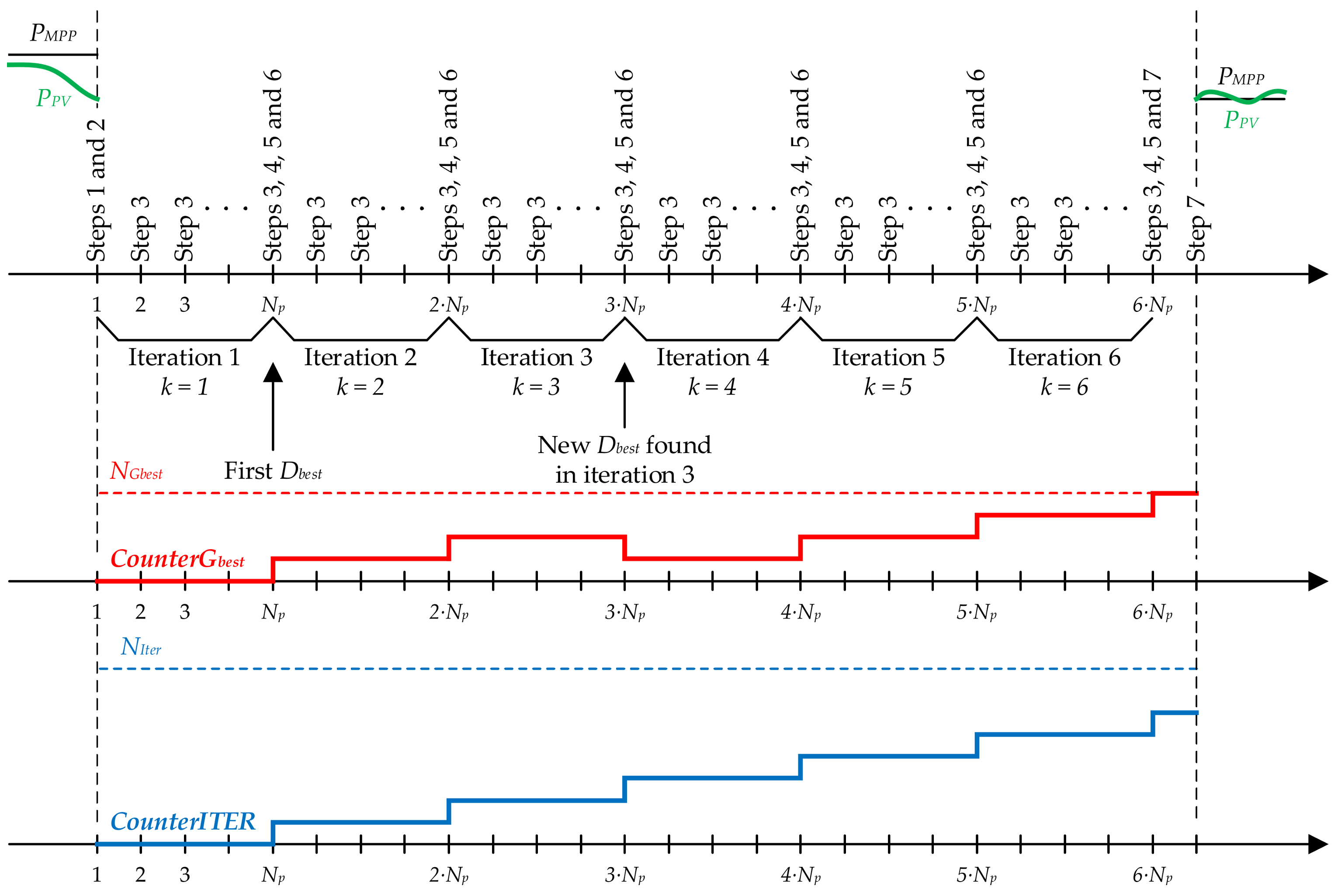
Figure 3 shows the timing of the proposed PSO-based MPPT algorithm. In the example of Figure 3, a decrease of PV output power triggers a new search of the GMPP and at the end of the third iteration an update of Dbest, PPV,Gbest occurs; NGbest is 4 and NIter is 8. Iterations from 3 to 6 are characterized by the same Dbest, thus the end of the sixth iteration triggers the check of the solution.
The time required for the search of the GMPP, T, is reported in Equation (5), and it depends on the number of particles to be evaluated in each iteration, Np, the number of iterations required to meet the convergence criterion, and the sampling time Ts. In order to avoid the measurement of the PV output power during transients, Ts has to be larger than the power converter settling time. It is easy to prove that the search process requires a quite long time interval in which the PV generator works at different power values, even far from the GMPP.
3. Test Case Modeling
3.1. Test Case PV System Model
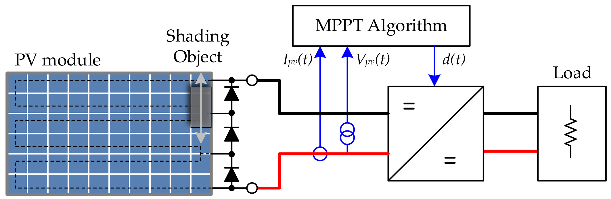
The test case PV system taken into account for simulating the MPPT algorithms is a simple off grid PV system that consists of a PV module, a boost DC/DC converter, a load resistor, and a MPPT controller. Figure 4 shows the diagram of the simulated off grid PV system. This model represents the MPPT test bench available at the SolarTechLab of the Department of Energy at Politecnico di Milano [24], which was used for a preliminary experimental test campaign carried out on 27 February and 3 March 2018. The MPPT algorithm controls the PV generator, regardless of the kind and the complexity of the PV system. Since the goal of this work is to investigate, by means of simulations, the capability of the MPPT controller to find the GMPP under partial and dynamic shading conditions, this simple off-grid PV system represents a general case suitable for this kind of research.
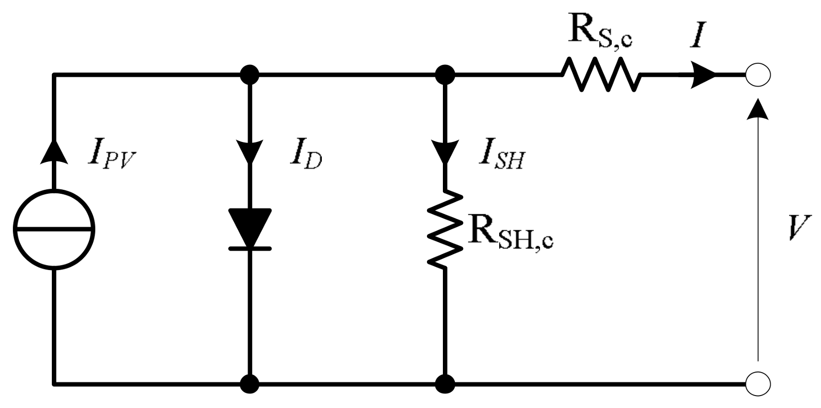
The PV module taken into account in this work is a monocrystalline S19.285 produced by Aleo Solar, whose ratings are reported in Table 1. It is made of 60 cells connected in series and three bypass diodes parallel connected to groups of 20 cells, which divide the PV module in three equal electrical sections. An active non-linear and time-varying element models the PV module. The PV module I-V curve is calculated combining the I-V curves of each cell and the I-V curves of each bypass diode in order to comply with the series and parallel electrical connection constraints. The I-V curve of each cell was calculated by using the five parameter mathematical model [26], whose equivalent circuit is reported in Figure 5. The five parameters that characterize this model are the light generated current (IPV), the leakage or reverse saturation current (I0), the diode quality factor (n), the series resistance (Rs) and the shunt resistance (Rsh). Referring to the equivalent electric circuit in Figure 5, the I-V curve of a PV cell can be expressed based on Kirchhoff’s current law, Ohm’s law, and the Shockley diode equation:
The light generated current as a function of irradiance, G, and cell temperature, TC, can be expressed as:
where the subscript ref stands for reference conditions, G is the irradiance, TC is the cell temperature and αISC is the temperature coefficient for short-circuit current. In most cases, reference values are measured at standard test conditions (STC), that is with Gref equal to 1000 W/m2, cell temperature equal to 25 °C and Air Mass equal to 1.5. In case of partial shading on a cell, its light generated current is directly proportional to the ratio of the unshaded area of the cell, Sunshaded, and its total surface, Scell. The unshaded area of each cell is calculated according to the shape of the shading object and its speed and position. The diode reverse saturation current can be expressed as:
where k is the Boltzmann constant (8.6173324∙10−5 eV∙K−1) and Eg is the bandgap energy of the silicon, that is temperature dependent and it is given, in eV, as:
The shunt resistance changes with absorbed solar radiation, and different equations can be found in literature. In this work, inversely proportional dependence of shunt resistance with irradiance is taken into account.
Variation of the ideality factor of the cell and the series resistance with irradiance and cell temperature are neglected.
The MPPT controller regulates the duty cycle according to the MPPT algorithm. As the MPPT controller always operates with the average PV voltage and current measured in the steady-state, the dynamics of the DC/DC converter, namely the voltage and current high frequency ripples, can be neglected. Moreover, MPPT controller regulates DC/DC converter input voltage and current regardless of its internal losses. In this context, the boost DC-DC converter is represented by its low-frequency ideal model, consisting of an ideal transformer, whose transformation ratio is:
where d(t) is the duty cycle, Vout(t) is the output voltage applied to the load resistor, and Vpv(t) is the input voltage applied to the PV module. According to the MPPT test facility available in the SolarTechLab, the resistance of the load resistor, Rload, is 37.5 Ω. At the PV module terminals, the load and the DC-DC converter can be replaced by an equivalent time-varying resistor, Req(t).
The solution of the electrical model is the intersection between the I-V curve representing the actual electrical behavior of the PV module and the load line representing the resistor.
3.2. Test Case Shading Scenarios Model
The simulated dynamic partial shading scenarios take into account the passage of a moving object close to the PV module, obstructing direct radiation and most of the diffuse radiation. In the model, it has been assumed that the irradiance is nil on the shaded area of the PV module. Four shading shapes are taken into account: a rectangular shape and three trapezoidal shapes. For each shape, three shading objects that are equal in height and differ only in length are considered, as summarized in Table 2. Taking the length of the solar cell edge as the unit of measurement, the dimensions of each shading object are 2 × 1, 3 × 1, and 4 × 1. The shading scenarios with rectangular shapes were also tested during the preliminary test campaign.
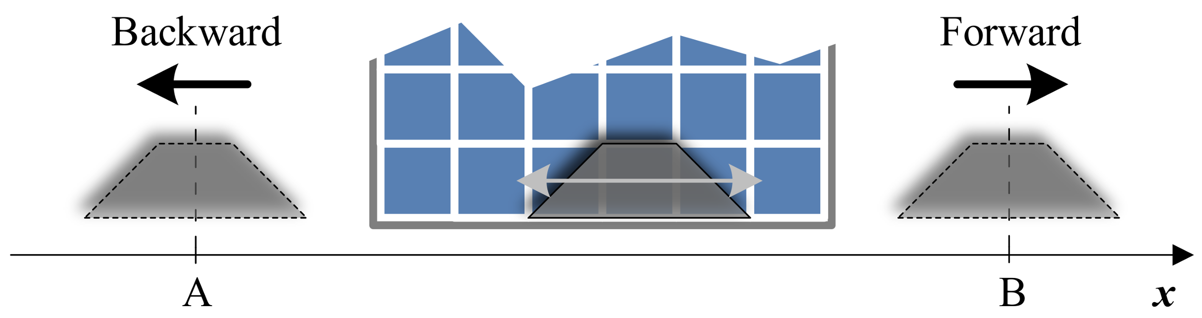
The shading object moves at a constant speed (4 cm/s) along the short edge of the PV module, as shown in Figure 6. The motion path is set between two points, A and B, respectively; the PV module is placed in the middle of the path. A motion cycle consists of a forward motion from A to B, a waiting time, and a backward motion from B to A.
The shapes and size of the shading objects have been defined to consider different dynamic partial shading cases, in terms of the number of completely and partially shaded cells at the same time, the rate of variation of the shaded area of PV cells, and the duration of the shading process. In a real world scenario, the shading process of a photovoltaic generator can be either deterministic or random. A deterministic partial shading process occurs in fixed PV installations; it is related to the motion of the sun in the sky and the fixed objects nearby to the PV generator [27], like trees, buildings, poles, etc., that can cause partial occlusion from the sun in some hours of the day. A deterministic partial shading process is usually a very slow process. A random partial shading process occurs both in fixed PV installations, due to the passage of clouds, and in stand-alone and moving applications, (e.g., cars or boats) because of motion. Fast dynamics characterize these types of shading. A random partial shading process is usually quite a fast process. The moving objects and their motion speed taken into account in this work allows us to simulate the shading processes that fall in the last case.
4. Test Case Simulations and Results
The test case simulations have been designed to verify the performance of the proposed PSO-based MPPT algorithm in different dynamic shading conditions and with different settings. The results obtained with the proposed PSO-based MPPT algorithm are compared with those generated by the use of widely used MPPT algorithms in the same conditions of dynamical shading. The performance of the proposed PSO-based MPPT algorithm as a function of the number of particles (population size) is investigated.
The following MPPT algorithms have been simulated for each shading scenario:
- Perturb and Observe (P&O—A);
- Variable Step Perturb and Observe (P&O—B);
- Three Point Weight Comparison (P&O—C);
- Incremental Conductance (IC);
- Constant Voltage (CV);
- Open Voltage (OV);
- Short Current Pulse (SC);
- PSO-based MPPT algorithm with 3 particles (PSO—3p);
- PSO-based MPPT algorithm with 4 particles (PSO—4p);
- PSO-based MPPT algorithm with 5 particles (PSO—5p).
For each shading object defined above and for each MPPT algorithm, two minutes of operation of the off grid PV system are simulated. The irradiance and cell temperature are constant during the whole simulation, equal to 800 W/m2 and 48 °C, respectively. Since MPPT algorithms regulate the PV generator both for irradiance changes and in case of dynamic partial shading, therefore constant irradiance is necessary to evaluate the behavior of the controller in the event of dynamic partial shading. Moreover, constant irradiance represents the environmental condition during a short time interval of a sunny day. The commonly used thermal model for predicting the temperature of PV cells in a PV module is based on the assumption that the difference between the cell and ambient temperature is proportional with the irradiance, thus constant irradiance corresponds to constant cell temperature. Partial shading on PV cells persists only for a few seconds: it is assumed that the cell temperature variation due to the passage of the moving object can be neglected.
The schedule of each partial shading simulation is organized as follows:
- At the beginning of the simulation (conventional time stamp t = 0 s), the PV module is unshaded and the MPP algorithm is in steady state.
- The dynamical shading produced by the object moving in forward direction starts 10 s after the beginning of the simulation (conventional time stamp t = 10 s). The dynamical partial shading condition ends as soon as the moving object’s rear-end leaves the PV module. Dynamic partial shading lasts for 31.7 s in case of 2 × 1 shading objects, for 35.7 s in case of 3 × 1 shading objects and for 39.7 s in case of 4 × 1 shading objects;
- The dynamical shading produced by the object moving in backward direction starts at the conventional time stamp t = 70 s. As in the case of forward motion, the dynamical partial shading lasts from 31.7 s to 39.7 s, depending on the length of shading objects.
- The simulation ends at the conventional time stamp t = 120 s.
Simulations have been performed by using a Matlab script that implements the calculation of the position of the moving object and the resulting shaded area of each cell, the electric model of the PV system, and the MPPT algorithm. The two minutes of operation of the off-grid PV system have been discretized using a sampling time of 50 ms. For each time sample:
- the position of the shading object and the resulting unshaded area of each cell of the PV module are calculated;
- the I–V curves of each PV cell and the I–V curve of the PV module are calculated and the electrical circuit is solved, namely VPV(n) and IPV(n) are calculated and PPV(n) is derived;
- one cycle of the MPPT algorithm is performed and the duty cycle is changed accordingly.
In order to compare the results of 120 simulation runs (10 MPPT algorithms and 12 shading scenarios) an appropriate Efficiency parameter of the MPPT algorithm has been defined and calculated. This efficiency parameter is represented by the ratio of the harvested energy and the maximum harvestable energy, and can be mathematically expressed by the following equations:
where VPV(t) and IPV(t) are the actual voltage and current at the terminals of PV generator, VMPP(t) and IMPP(t) are the coordinates of the actual GMPP.
4.1. Results: Rectangular Shape
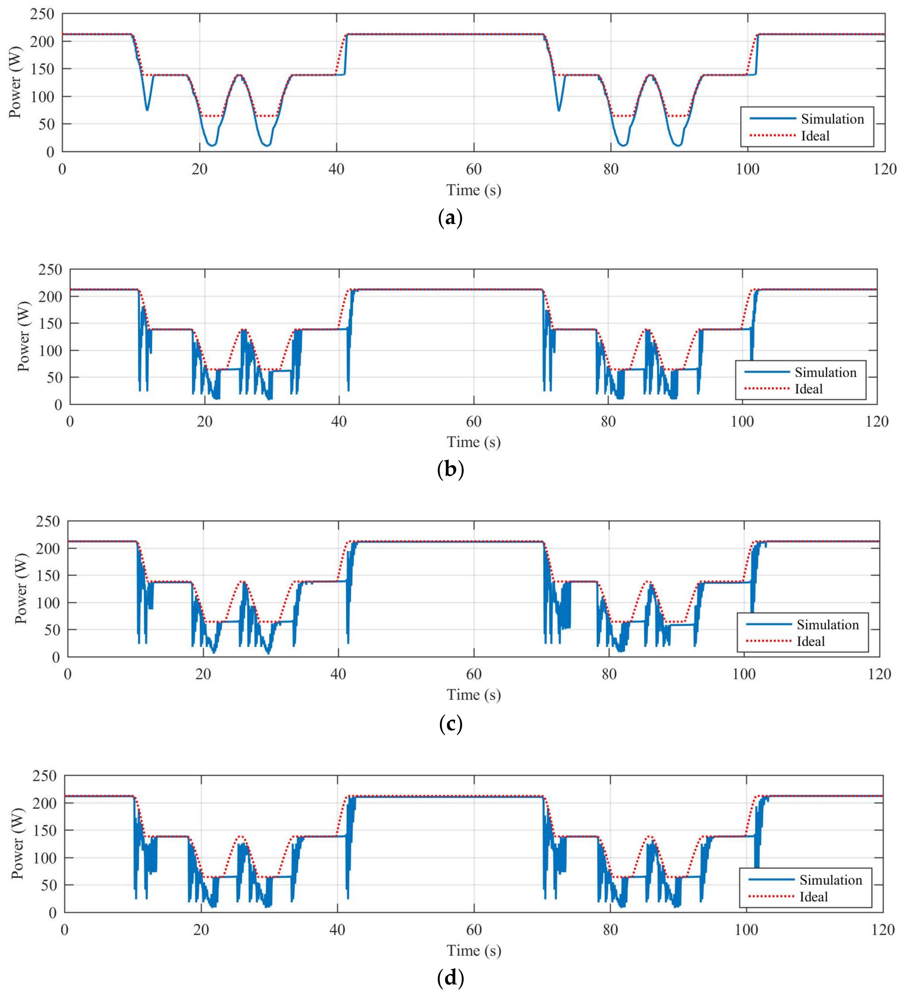
Table 3 reports the efficiency calculated for all the dynamical shading scenarios characterized by a rectangular shape’s objects; the results obtained both from simulations and from preliminary experimental tests are reported. In the latter case, the plane of array global irradiance and the PV cell temperature during each test were recorded by the weather station installed in the SolarTechLab, and the maximum harvestable energy was estimated accordingly. A stepper motor moves the carriage with the shading object at constant speed along a rail and the signals from two optical sensors on the rail, synchronized with the shadow produced by the shape on the PV module, trigger the beginning and the ending of the partial shading process [24]. Figure 7 shows, as example, the diagrams of the harvested power (solid blue line) and maximum harvestable power (dotted red line): these are obtained in case of dynamical shading caused by the rectangular 2 × 1 shading object and controlling the off grid PV system, with the best performing traditional MPPT algorithm (P&O—B) and the proposed PSO-based MPPT algorithm characterized by three, four, and five agents respectively.
The comparison with these diagrams highlight the benefits and drawbacks of the proposed PSO-based MPPT algorithm under a quite general case of a dynamic partial shading scenario. The PSO-based MPPT algorithm reacts immediately to any variation in the PV output power caused by dynamic shading, while Variable Step Perturb and Observe requires quite a long time to move to another peak, and during this process could get stuck in a specific (local) peak. The latter characteristics, that are a common feature of the hill-climbing methods, can be both a benefit or a drawback, depending on how the shade moves on the surface of the PV module. On the other hand, the PSO-based MPPT algorithm always tracks the GMPP, but the search of the GMPP requires quite a long time interval in which the PV generator is operated at different power values, even far from the GMPP, thus reducing conversion efficiency. Moreover, the PSO-based MPPT algorithm is not suitable for tracking the GMPP when its power changes during scan.
The efficiency gap between the best PSO-based MPPT algorithm and the best hill climbing technique varies from 2.71% (3 × 1, P&O—A vs. PSO—3p) to 5.95% (4 × 1, P&O—A vs. PSO—5p). This behavior is strictly related to the long time required to track the GMPP, also combined with the inadequacy of the PSO-based MPPT method when the power of the GMPP changes during the scan phase.
The comparison among the results generated by the PSO-based MPPT algorithm with a variable number of agents shows that there is no specific rule to determine the optimum number of particles. As the number of particles increases, there is a tendency to reduce the number of iterations required to track the GMPP, but each iteration requires more time to evaluate the fitness function.
4.2. Results: Trapezoidal-A Shape
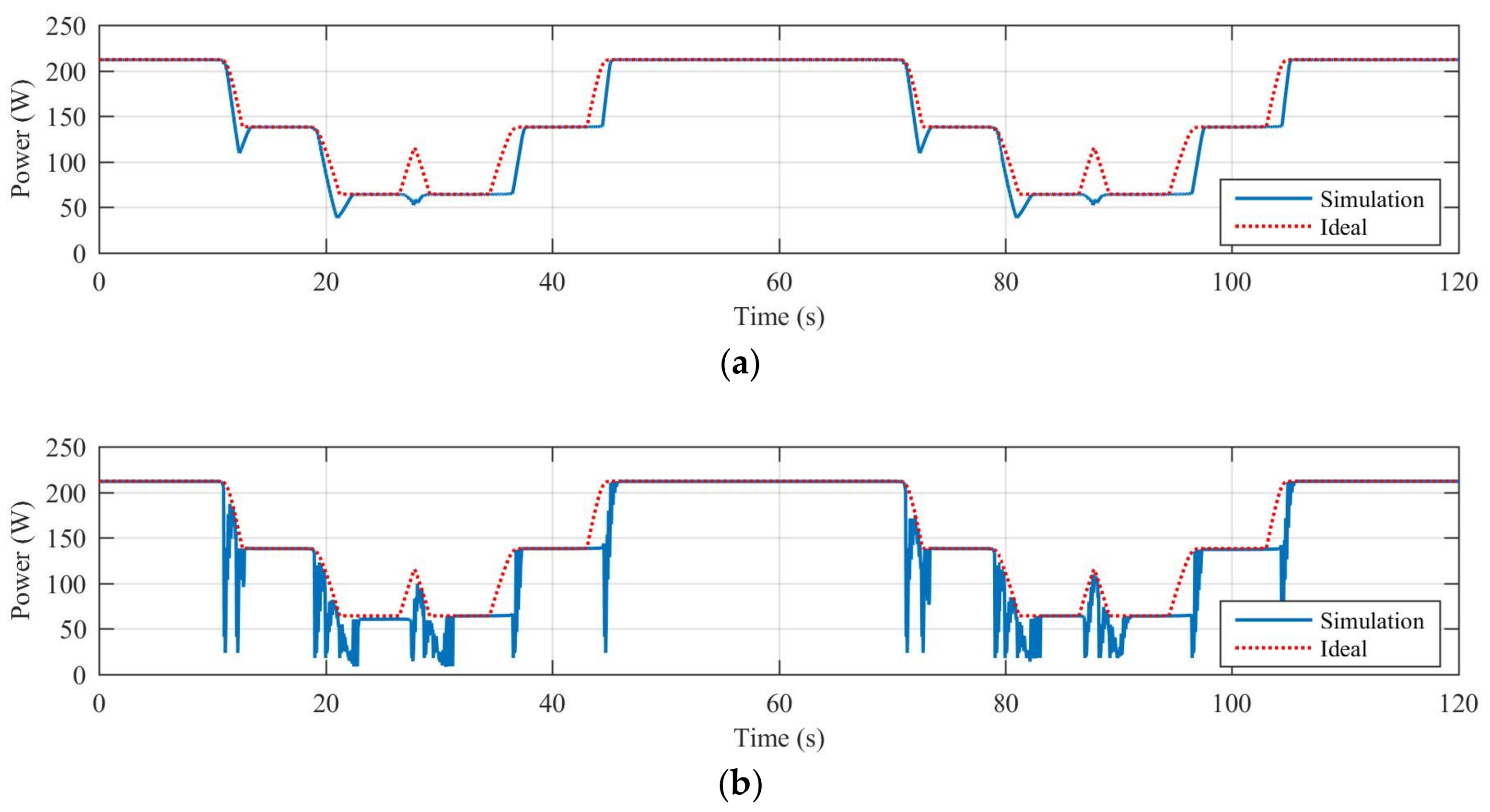
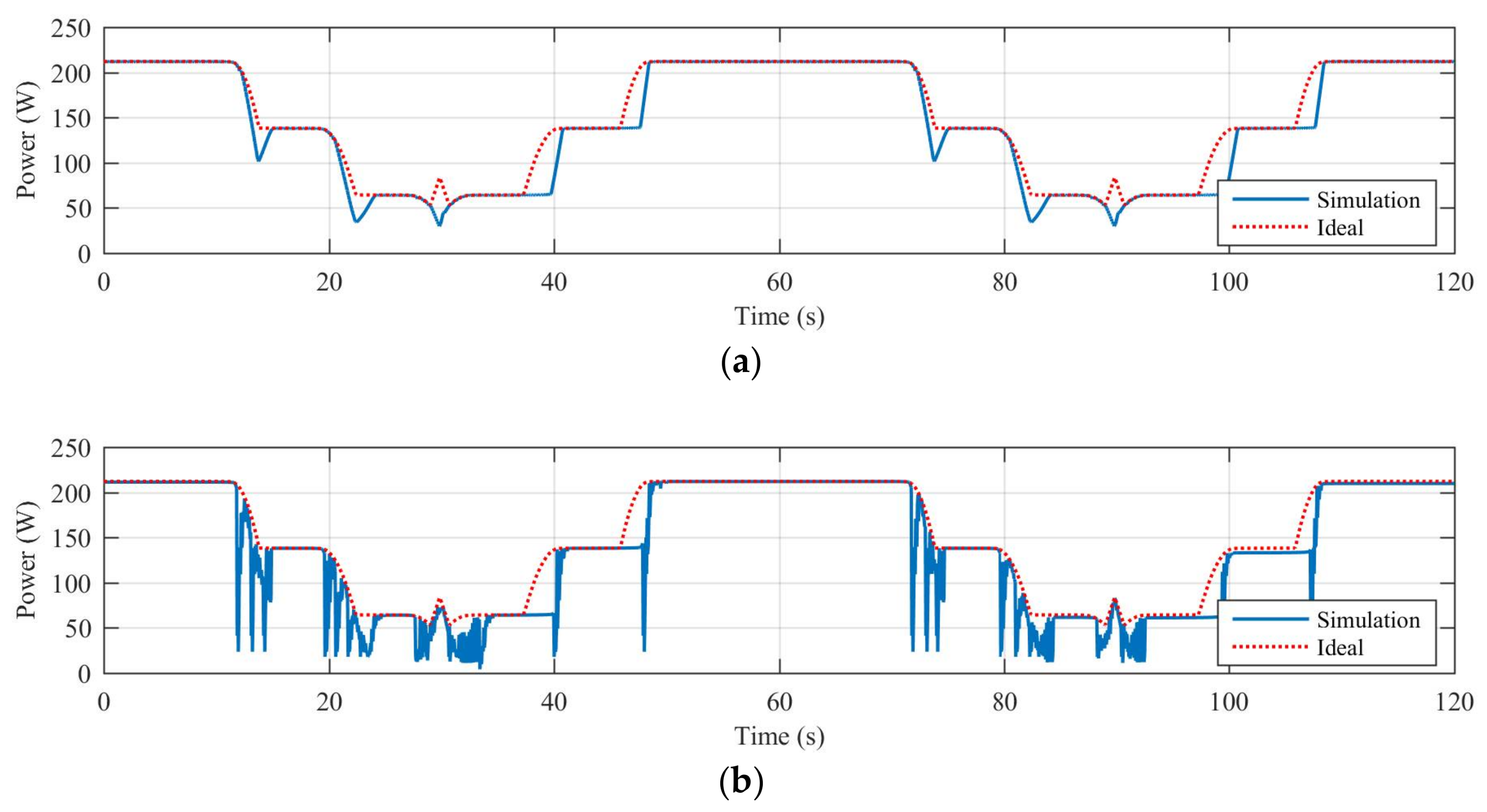
Table 4 reports the efficiency calculated for all the dynamical shading scenarios characterized by Trapezoidal-A shape’s objects. Figure 8 shows, as example, the diagrams of the harvested power (solid blue line) and maximum harvestable power (dotted red line) obtained in case of dynamical shading caused by the trapezoidal-A shape 3 × 1 shading object and controlling the off grid PV system, with the best performing traditional MPPT algorithm (P&O—A) and the best performing PSO-based MPPT algorithm (PSO—3p).
The obtained results are very similar to those obtained in the case of dynamical shading generated by rectangular objects. In this case the efficiency of the best PSO-based MPPT algorithm is again lower than the best hill climbing technique, namely 2.38% (2 × 1, P&O—B vs. PSO—3p) and 4.82% (3 × 1, P&O—A vs. PSO—3p) less respectively, and no specific rule determines the optimum number of particles.
4.3. Results: Trapezoidal-B Shape
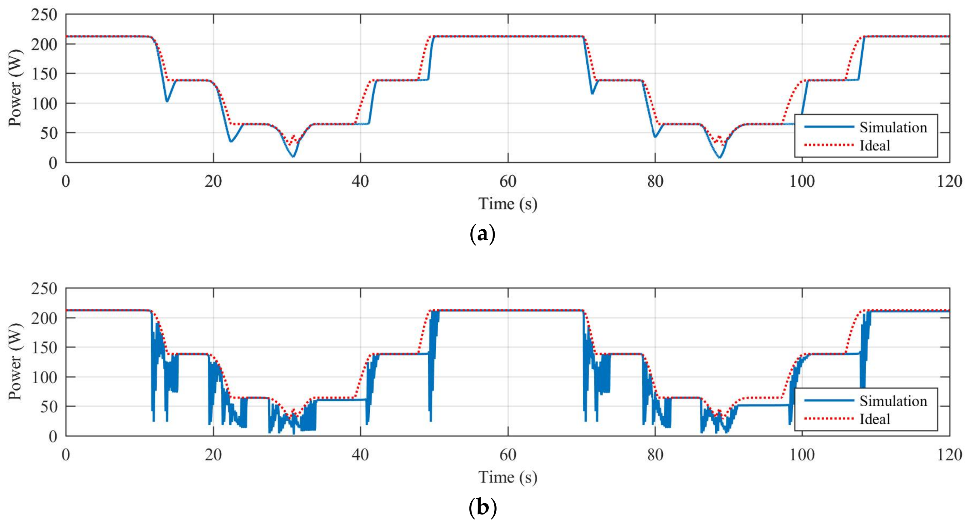
Table 5 reports the efficiency calculated for all the dynamical shading scenarios characterized by Trapezoidal-B shape’s objects. Figure 9 shows, as example, the diagrams of the harvested power (solid blue line) and maximum harvestable power (dotted red line) obtained in case of dynamical shading caused by the trapezoidal-A shape 4 × 1 shading object and controlling the off grid PV system, with the best performing traditional MPPT algorithm (P&O—A) and the best performing PSO-based MPPT algorithm (PSO—3p).
The obtained results are very similar to those obtained in the previous cases of dynamical shading. The efficiency of the best PSO-based MPPT algorithm ranges from a 3.42% (4 × 1, P&O—A vs. PSO—3p) to a 4.51% (2 × 1, P&O—B vs. PSO—3p) lower than the best hill climbing technique.
4.4. Results: Trapezoidal-C Shape
Finally, Table 6 reports the efficiency calculated for all the dynamical shading scenarios characterized by the Trapezoidal-C shape’s objects. Figure 10 shows, as example, the diagrams of the harvested power (solid blue line) and maximum harvestable power (dotted red line) obtained in case of dynamical shading caused by the trapezoidal-A shape 4 × 1 shading object and controlling the off grid PV system, with the best performing traditional MPPT algorithm (P&O—A) and the best performing PSO-based MPPT algorithm (PSO—5p).
The obtained results are again quite similar to those obtained in the previous cases. The efficiency of the best PSO-based MPPT algorithm in this last case ranges from 2.86% (3 × 1, P&O—A vs. PSO—3p) to 5.18% (2 × 1, P&O—B vs. PSO—5p) lower than the best hill climbing technique, confirming once more the same performance behavior, which in these simulations is independent of the particular applied dynamic shading conditions.
5. Conclusions
Solar energy remains one of the best choices among renewables, being an inexhaustible energy source available everywhere with zero carbon emissions, but optimization in the performance of PV systems has become a priority.
This paper has proposed a comparison of traditional MPPT algorithms with an evolutionary based computational technique able to optimize extraction of solar power under dynamic environmental conditions. Partial shading conditions in different shape, size, and dynamics have been simulated, thus proving that dynamic conditions always represent a critical task for maximum power extraction. The effective use of a PSO-based algorithm has demonstrated that computational intelligence techniques can provide effective methods only if the population size increases, but under dynamic shading conditions computational time cannot be a negligible issue related to high conversion efficiency tasks. Moreover, this study has shown that PSO-based MPPT algorithm guarantees to effectively reach the global MPP, but the search of the global power point requires significant computational time, thus compromising conversion efficiency, especially in fast dynamic conditions.
Future works will include further improvements in the efficiency of the algorithm by reducing the computational time taken for scanning, choosing a more efficient approach that also considers hybrid strategies, and a deep experimental test campaign.
Author Contributions
Alberto Dolara has been the corresponding author and with Francesco Grimaccia contributed to the manuscript composition and test scenario developments. Alberto Dolara, Emanuele Ogliari and Marco Mussetta also implemented and ran the algorithms in the Matlab environment. Sonia Leva supervised the manuscript composition and the experimental validation, carried out at the Department of Energy, Politecnico di Milano (Italy).
Conflicts of Interest
The authors declare no conflict of interest.
Nomenclature
| CI | Computational Intelligence |
| CV | Constant Voltage |
| DC/DC | Direct Current to Direct Current |
| GMPP | Global Maximum Power Point |
| IC | Incremental Conductance |
| MPP | Maximum Power Point |
| MPPT | Maximum Power Point Tracking |
| OV | Open Voltage |
| PSO | Particle Swarm Optimization |
| PV | Photovoltaic |
| P&O | Perturb and Observe |
| SC | Short Current Pulse |
References
- Hernandez, R.R.; Easter, S.B.; Murphy-Mariscal, M.L.; Maestre, F.T.; Tavassoli, M.; Allen, E.B.; Barrows, C.W.; Belnap, J.; Ochoa-Hueso, R.; Ravi, S.; et al. Environmental impacts of utility-scale solar energy. Renew. Sustain. Energy Rev. 2014, 29, 766–779. [Google Scholar] [CrossRef]
- Turney, D.; Fthenakis, V. Environmental impacts from the installation and operation of large-scale solar power plants. Renew. Sustain. Energy Rev. 2011, 15, 3261–3270. [Google Scholar] [CrossRef]
- Karavas, C.S.; Arvanitis, K.G.; Kyriakarakos, G.; Piromalis, D.D.; Papadakis, G. A novel autonomous PV powered desalination system based on a DC microgrid concept incorporating short-term energy storage. Sol. Energy 2018, 159, 947–961. [Google Scholar] [CrossRef]
- Dolara, A.; Grimaccia, F.; Magistrati, G.; Marchegiani, G. Optimization Models for islanded micro-grids: A comparative analysis between linear programming and mixed integer programming. Energies 2017, 10, 1–20. [Google Scholar] [CrossRef]
- Grimaccia, F.; Leva, S.; Mussetta, M.; Ogliari, E. ANN sizing procedure for the day-ahead output power forecast of a PV plant. Appl. Sci. 2017, 7, 622. [Google Scholar] [CrossRef]
- Dolara, A.; Leva, S.; Manzolini, G.; Ogliari, E. Investigation on performance decay on photovoltaic modules: Snail trails and cell microcracks. IEEE J. Photovolt. 2014, 4, 1204–1211. [Google Scholar] [CrossRef]
- Dolara, A.; Lazaroiu, G.C.; Leva, S.; Manzolini, G.; Votta, L. Snail Trails and Cell Microcrack Impact on PV Module Maximum Power and Energy Production. IEEE J. Photovolt. 2016, 6, 1269–1276. [Google Scholar] [CrossRef]
- Aghaei, M.; Grimaccia, F.; Gonano, C.A.; Leva, S. Innovative Automated Control System for PV Fields Inspection and Remote Control. IEEE Trans. Ind. Electron. 2015, 62, 7287–7296. [Google Scholar] [CrossRef]
- Grimaccia, F.; Leva, S.; Niccolai, A. PV plant digital mapping for modules’ defects detection by unmanned aerial vehicles. IET Renew. Power Gener. 2017, 11, 1221–1228. [Google Scholar] [CrossRef]
- Siddique, N.; Adeli, H. Computational Intelligence: Synergies of Fuzzy Logic, Neural Networks and Evolutionary Computing; John Wiley & Sons: Chichester, UK, 2013. [Google Scholar]
- Coello, C.A.; Lechuga, M.S. MOPSO: A proposal for multiple objective particle swarm optimization. In Proceedings of the Congress on Evolutionary Computation (CEC’02), Honolulu, HI, USA, 12–17 May 2002. [Google Scholar]
- Berrera, M.; Dolara, A.; Faranda, R.; Leva, S. Experimental test of seven widely-adopted MPPT algorithms. In Proceedings of the 2009 IEEE Bucharest PowerTech: Innovative Ideas Toward the Electrical Grid of the Future, Bucarest, Romania, 28 June–2 July 2019. [Google Scholar]
- Prasanth Ram, J.; Sudhakar Babu, T.; Rajasekar, N. A comprehensive review on solar PV maximum power point tracking techniques. Renew. Sustain. Energy Rev. 2017, 67, 826–847. [Google Scholar] [CrossRef]
- Salas, V.; Olías, E.; Barrado, A.; Lázaro, A. Review of the maximum power point tracking algorithms for stand-alone photovoltaic systems. Sol. Energy Mater. Sol. Cells 2006, 90, 1555–1578. [Google Scholar] [CrossRef]
- Karami, N.; Moubayed, N.; Outbib, R. General review and classification of different MPPT Techniques. Renew. Sustain. Energy Rev. 2017, 68, 1–18. [Google Scholar] [CrossRef]
- Dolara, A.; Leva, S.; Magisrtrati, G.; Mussetta, M.; Ogliari, E. A novel MPPT algorithm for photovoltaic systems under dynamic partial shading-Recurrent scan and track method. In Proceedings of the 5th IEEE International Conference on Renewable Energy Research and Applications, Birmingham, UK, 20–23 November 2016. [Google Scholar]
- Kollimalla, S.K.; Mishra, M.K. Variable Perturbation Size Adaptive P&O MPPT Algorithm for Sudden Changes in Irradiance. IEEE Trans. Sustain. Energy 2014, 5, 718–728. [Google Scholar]
- Ananthi, C.; Kannapiran, B. Improved design of sliding-mode controller based on the incremental conductance MPPT algorithm for PV applications. In Proceedings of the 2017 IEEE International Conference on Electrical, Instrumentation and Communication Engineering, Karur, India, 27–28 April 2017. [Google Scholar]
- Ma, J.; Man, K.L.; Ting, T.O.; Zhang, N.; Lei, C.; Wong, N. A Hybrid MPPT Method for Photovoltaic Systems via Estimation and Revision Method. In Proceedings of the IEEE International Symposium on Circuits and Systems (ISCAS), Beijing, China, 19–23 May 2013. [Google Scholar]
- Sher, H.A.; Addoweesh, K.E.; Haddad, K.A. An Efficient and Cost-Effective Hybrid MPPT Method for a Photovoltaic Flyback Micro-Inverter. IEEE Trans. Sustain. Energy 2017, PP, 1. [Google Scholar] [CrossRef]
- Hanafiah, S.; Ayad, A.; Hehn, A.; Kennel, R. A hybrid MPPT for quasi-Z-source inverters in PV applications under partial shading condition. In Proceedings of the 11th IEEE International Conference on Compatibility, Power Electronics and Power Engineering, Cadiz, Spain, 4–6 April 2017. [Google Scholar]
- Ishaque, K.; Salam, Z. A Deterministic Particle Swarm Optimization Maximum Power Point Tracker for Photovoltaic System under Partial Shading Condition. IEEE Trans. Ind. Electron. 2013, 60, 3195–3206. [Google Scholar] [CrossRef]
- Hohm, D.P.; Ropp, M.E. Comparative Study of Maximum Power Point Tracking Algorithms Using an Experimental, Programmable, Maximum Power Point Tracking Test Bed. In Proceedings of the IEEE Photovoltaic Specialist Conference, Anchorage, AK, USA, 15–22 September 2000. [Google Scholar]
- Aghaei, M.; Dolara, A.; Grimaccia, F.; Leva, S.; Kania, D.; Borkowski, J. Experimental Comparison of MPPT Methods for PV Systems Under Dynamic Partial Shading Conditions. In Proceedings of the 16th International Conference on Environment and Electrical Engineering, Florence, Italy, 7–10 June 2016. [Google Scholar]
- Dolara, A.; Lazaroiu, G.C.; Leva, S.; Manzolini, G. Experimental investigation of partial shading scenarios on PV (photovoltaic) modules. Energy 2013, 55, 466–475. [Google Scholar] [CrossRef]
- Dolara, A.; Leva, S.; Manzolini, G. Comparison of different physical models for PV power output prediction. Sol. Energy 2015, 119, 83–99. [Google Scholar] [CrossRef] [Green Version]
- Dolara, A.; Lazaroiu, G.C.; Ogliari, E. Efficiency analysis of PV power plants shaded by MV overhead lines. Int. J. Energy Environ. Eng. 2016, 7, 115–123. [Google Scholar] [CrossRef]
Figure 1.
Flowchart of Particle Swarm Optimization (PSO)-based Maximum Power Point (MPP) tracking method.
Figure 1.
Flowchart of Particle Swarm Optimization (PSO)-based Maximum Power Point (MPP) tracking method.

Figure 2.
Flowchart of the functions (a) “Check for power changes” and (b) “Check GMPP”.

Figure 3.
Timing of the proposed PSO-based Maximum Power Point Tracking (MPPT) algorithm.

Figure 4.
Diagram of the simulated off grid photovoltaic (PV) system.

Figure 5.
Diagram of the simulated off grid PV system.

Figure 6.
Diagram of the motion cycle: the shading object is moved forward and backward in one cycle.
Figure 6.
Diagram of the motion cycle: the shading object is moved forward and backward in one cycle.

Figure 7.
Rectangular shape—2 × 1: (a) P&O—B; (b) PSO 3 particles; (c) PSO 4 particles; (d) PSO 5 particles.
Figure 7.
Rectangular shape—2 × 1: (a) P&O—B; (b) PSO 3 particles; (c) PSO 4 particles; (d) PSO 5 particles.

Figure 8.
Trapezoidal-A shape—3 × 1: (a) P&O—A; (b) PSO 3 particles.

Figure 9.
Trapezoidal-B shape—4 × 1: (a) P&O—A; (b) PSO 3 particles.

Figure 10.
Trapezoidal-C shape—4 × 1: (a) P&O—A; (b) PSO 5 particles.


Table 1.
PV module electrical data.
| Electrical Data | STC (1) | NOCT (2) | |
|---|---|---|---|
| Rated Power | PMPP (W) | 285 | 208 |
| Rated Voltage | VMPP (V) | 31.3 | 28.4 |
| Rated Current | IMPP (A) | 9.10 | 7.33 |
| Open-Circuit Voltage | VOC (V) | 39.2 | 36.1 |
| Short-Circuit Current | ISC (A) | 9.73 | 7.87 |
(1) Electrical values measured under Standard Test Conditions: 1000 W/m2, cell temperature 25 °C, AM 1.5; (2) Electrical values measured under Nominal Operating Conditions of cells: 800 W/m2, ambient temperature 20 °C, AM 1.5, wind speed 1 m/s, NOCT: 48 °C (nominal operating cell temperature).
Table 2.
Shading objects.
| Size | Rectangular | Trapezoidal-A | Trapezoidal-B | Trapezoidal-C |
|---|---|---|---|---|
| 2 × 1 |  |  |  |  |
| 3 × 1 |  |  |  |  |
| 4 × 1 |  |  |  |  |
Table 3.
Efficiency—Rectangular shapes (simulations and preliminary experimental tests).
| MPPT | Efficiency | |||||
|---|---|---|---|---|---|---|
| 2 × 1 | 3 × 1 | 4 × 1 | ||||
| Sim. | Exp. | Sim. | Exp. | Sim. | Exp. | |
| Perturb & Observe—A | 95.34% | 93.66% | 96.19% | 97.93% | 95.37% | 95.41% |
| Perturb & Observe—B | 95.85% | 95.54% | 93.01% | 93.29% | 94.23% | 92.76% |
| Perturb & Observe—C | 93.40% | 91.04% | 94.34% | 91.94% | 93.48% | 94.52% |
| Incremental Conductance | 94.92% | 92.74% | 95.88% | 94.97% | 95.28% | 95.68% |
| Constant Voltage | 68.10% | 69.37% | 64.56% | 65.38% | 60.18% | 60.09% |
| Open Voltage | 79.33% | 78.77% | 73.56% | 73.15% | 71.38% | 71.74% |
| Short Current Pulse | 93.87% | 93.17% | 93.59% | 94.25% | 91.33% | 89.30% |
| PSO—3 particles | 92.54% | 89.40% | 93.48% | 91.35% | 88.77% | 85.59% |
| PSO—4 particles | 91.55% | 91.65% | 90.84% | 88.02% | 85.66% | 82.86% |
| PSO—5 particles | 90.80% | 90.08% | 91.76% | 88.92% | 89.42% | 89.60% |
Table 4.
Efficiency—Trapezoidal-A shapes (simulations).
| MPPT | Efficiency | ||
|---|---|---|---|
| 2 × 1 | 3 × 1 | 4 × 1 | |
| Perturb & Observe—A | 95.37% | 95.82% | 95.95% |
| Perturb & Observe—B | 97.59% | 94.68% | 95.30% |
| Perturb & Observe—C | 93.28% | 94.26% | 93.69% |
| Incremental Conductance | 96.03% | 94.73% | 94.72% |
| Constant Voltage | 69.90% | 66.41% | 62.19% |
| Open Voltage | 69.22% | 73.29% | 72.17% |
| Short Current Pulse | 93.75% | 93.47% | 91.42% |
| PSO—3 particles | 92.77% | 93.44% | 89.71% |
| PSO—4 particles | 87.89% | 90.91% | 90.64% |
| PSO—5 particles | 90.34% | 91.57% | 91.36% |
Table 5.
Efficiency—Trapezoidal-B shapes (simulations).
| MPPT | Efficiency | ||
|---|---|---|---|
| 2 × 1 | 3 × 1 | 4 × 1 | |
| Perturb & Observe—A | 97.39% | 94.52% | 95.41% |
| Perturb & Observe—B | 97.91% | 95.81% | 91.14% |
| Perturb & Observe—C | 95.62% | 92.58% | 93.47% |
| Incremental Conductance | 97.06% | 92.94% | 92.83% |
| Constant Voltage | 85.98% | 69.60% | 66.15% |
| Open Voltage | 85.32% | 68.92% | 75.62% |
| Short Current Pulse | 91.98% | 91.77% | 91.17% |
| PSO—3 particles | 93.40% | 90.47% | 91.99% |
| PSO—4 particles | 92.34% | 91.82% | 90.11% |
| PSO—5 particles | 91.25% | 89.27% | 89.30% |
Table 6.
Efficiency—Trapezoidal-C shapes (simulations).
| MPPT | Efficiency | ||
|---|---|---|---|
| 2 × 1 | 3 × 1 | 4 × 1 | |
| Perturb & Observe—A | 95.06% | 95.48% | 95.64% |
| Perturb & Observe—B | 97.65% | 94.10% | 95.22% |
| Perturb & Observe—C | 93.35% | 93.82% | 93.19% |
| Incremental Conductance | 95.34% | 94.16% | 94.31% |
| Constant Voltage | 71.59% | 67.37% | 63.15% |
| Open Voltage | 70.92% | 73.81% | 72.42% |
| Short Current Pulse | 93.01% | 92.81% | 91.77% |
| PSO—3 particles | 91.07% | 92.62% | 88.54% |
| PSO—4 particles | 91.78% | 92.02% | 90.40% |
| PSO—5 particles | 92.47% | 91.61% | 91.10% |
© 2018 by the authors. Licensee MDPI, Basel, Switzerland. This article is an open access article distributed under the terms and conditions of the Creative Commons Attribution (CC BY) license (http://creativecommons.org/licenses/by/4.0/).
Share and Cite
MDPI and ACS Style
Dolara, A.; Grimaccia, F.; Mussetta, M.; Ogliari, E.; Leva, S. An Evolutionary-Based MPPT Algorithm for Photovoltaic Systems under Dynamic Partial Shading. Appl. Sci. 2018, 8, 558. https://0-doi-org.brum.beds.ac.uk/10.3390/app8040558
AMA Style
Dolara A, Grimaccia F, Mussetta M, Ogliari E, Leva S. An Evolutionary-Based MPPT Algorithm for Photovoltaic Systems under Dynamic Partial Shading. Applied Sciences. 2018; 8(4):558. https://0-doi-org.brum.beds.ac.uk/10.3390/app8040558
Chicago/Turabian StyleDolara, Alberto, Francesco Grimaccia, Marco Mussetta, Emanuele Ogliari, and Sonia Leva. 2018. "An Evolutionary-Based MPPT Algorithm for Photovoltaic Systems under Dynamic Partial Shading" Applied Sciences 8, no. 4: 558. https://0-doi-org.brum.beds.ac.uk/10.3390/app8040558
Note that from the first issue of 2016, this journal uses article numbers instead of page numbers. See further details here.