Reconstruct Recurrent Neural Networks via Flexible Sub-Models for Time Series Classification


Laboratory of Automatic Target Recognition, College of Electronic Science, National University of Defense Technology (NUDT), Changsha 410073, China
*
Author to whom correspondence should be addressed.
Appl. Sci. 2018, 8(4), 630; https://0-doi-org.brum.beds.ac.uk/10.3390/app8040630
Submission received: 21 March 2018
/
Revised: 15 April 2018
/
Accepted: 16 April 2018
/
Published: 18 April 2018
Abstract
:Recurrent neural networks (RNNs) remain challenging, and there is still a lack of long-term memory or learning ability in sequential data classification and prediction. In this paper, we propose a flexible recurrent model, BIdirectional COnvolutional RaNdom RNNs (BICORN-RNNs), incorporating a series of sub-models: random projection, convolutional operation, and bidirectional transmission. These subcategories advance classification accuracy, which was limited by the gradient vanishing and the exploding problem. Experiments on public time series datasets demonstrate that our proposed method substantially outperforms a variety of existing models. Furthermore, the coordination of the accuracy and efficiency concerning a variety of factors, including SNR, length, data missing, and overlapping, is also discussed.
1. Introduction
As an important problem of data mining, time series classification (TSC) has been maturely used in many fields, such as natural language processing, biomedical diagnosis, and financial analysis [1,2,3,4]. However, continuous research of TSC has never stagnated because of its complications: long-standing large data scale, high dimension, and continuous updating of data stream. Many researchers have proposed various methods and achieved state-of-the-art results, promoting classification issues to suit deeper task requirements. As seen from numerous studies, TSC techniques mainly include these categories: distance-based methods, feature-based methods, and artificial neural network (ANN)-based methods [5].
For distance-based methods, using particular metrics to measure the similarity between two series is effective in comprehensive applications. The most representative metric is the nearest neighbor (1-NN or k-NN) [6,7,8] algorithm, which is based on Euclidean distance [9] and dynamic time warping (DTW) [10]. However, Euclidean distance is sensitive to noise jamming and phase drift, and cannot deal with data of unequal-length directly. Additionally, DTW has the disadvantage of large computation costs in dynamic programming. Throughout various previous works, distance measurements based on similarity have regrettably shown a poor level of interpretation, and pose difficulties vis a vis bringing about a high degree of reliability.
Traditional feature-based classification methods can also be applied to time series data with less computational complexity. Both simple statistical features, such as mean and variance, and complex features, such as shapelets [11] and random forest [12], are mutually compatible to describe data characteristics in different scenarios [13,14]. However, the classification accuracy of this method depends heavily on the quality of the hand-crafted features. In contrast to other data types, for the time series data it is difficult to construct proper features in human intuition to capture the all characteristics. So, the classification performance of feature-based methods is generally inferior to distance-based ones.
Thus, we considered the use of ANN-based methods to learn an appropriate set of features automatically through neural transmission, when the feature is difficult to be described and extracted manually. Different from “Prior knowledge is the only decisive factor” in the above methods, in general, ANNs models are less specific and more adaptive. ANNs take the principle “Infer knowledge from the data” to the extreme [15]. Prosperous improved networks have been proposed, e.g. time delay neural networks (TDNNs) [16] and recurrent neural networks (RNNs) [17], providing more promising options to break the restrictions of dealing only with static data patterns.
RNN is inspired by the recurrent connection of neurons, and exploits iterative function loops to store and transmit historical information dynamically. Actually, the original process is very brittle because it has little feasible access to further information over a long period of time. In recent years, some intricate techniques have led to impressive results, such as gradient clipping [18], modifying activation function [19], long short-term memory (LSTM) [20,21], and identity initialization [22]. However, few research efforts have attempted flexible RNNs designs in the area of time series. It is also a critical flaw that the original RNNs cannot decide what consequential information needs to be remembered continuously, and what inconsequential information needs to be ignored gradually, in practical time series data [23].
Our purpose is to propose further improvement on the RNNs classifier, in order to expand the learning ability of essential information in long-term dependencies by projecting the predictions of previous outputs randomly, without complex training techniques. The flexible combination of the random projection, convolutional operation, and bidirectional transmission, “BICORN”, which is the core of our reform, provides a promising solution to the key issue: “remember or ignore”. In addition, we make an effort to compare our model to several classical classifiers, and we discuss the effects of several factors impacting the capability of learning temporal dependencies.
The remainder of the paper is organized as follows: Section 2 introduces the TSC tasks based on RNNs, and describes gradient problems when training networks. In Section 3, we propose BICORN-RNNs models composed of three parts, whilst we analyze the combination of these alternatives. We present experimental results of the proposed classifiers with the public datasets, and simulate the effects of several factors in Section 4. We conclude with a discussion in Section 5.
2. Problem Description
In this section, we describe the training and testing processes of TSC based on RNNs. We then analyze the long-term learning defect about gradient problem.
2.1. RNNs Structure
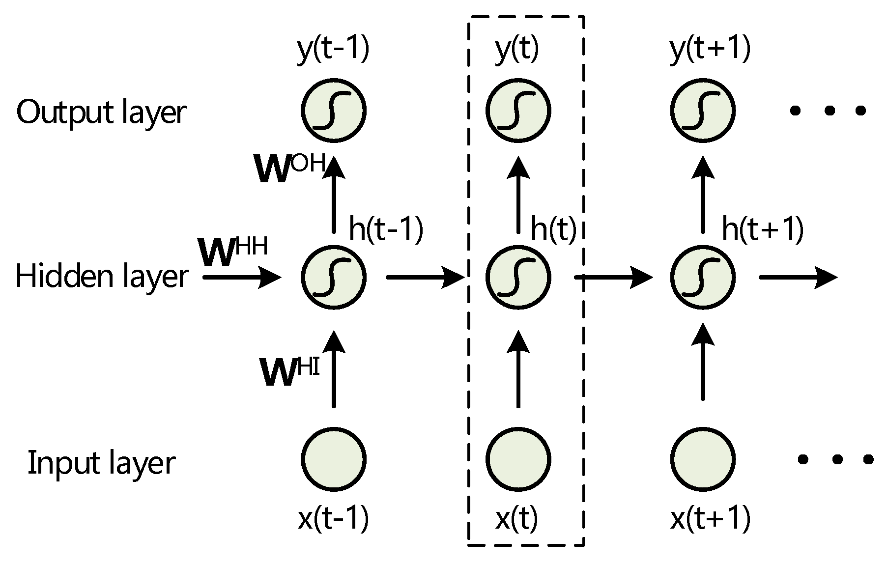
A discrete-time dynamical RNN system can project the entire previous inputs to each output. In principle, a standard Elman’s RNN [17] consists of input layer X, output layer Y, and hidden layer H. In order to describe RNNs compactly, here we focus on their simple network architecture with only one hidden layer.
The input vector X = [x(1), x(2),…, x(T)] is given as a discrete sequence with length of T, where (),and Y = [y(1), y(2),…,y(t)] is output vector, which is calculated via hidden states H = [h(1), h(2),…, h(t)], as shown in Figure 1. We use the subscript i to represent the i-th component of a vector at the t-th time-step, and t is related to temporal dynamical characteristics of RNNs. Thus, RNNs can be described as:
where f and g are the nonlinear element-wise activation function and output function, which are more powerful than linear combination functions in determining nonlinear classification boundaries. These parameters , , denote the input weight matrix, the recurrent weight matrix, and the output weight matrix respectively. , are bias weight matrices. I and O denote the number of input and output units of RNNs, which are decided by the format of input sequences and the number of target classes. The number of hidden neurons H in the only hidden layer is set manually when achieving network initialization, and the number of hidden neurons is fixed during training if there is no growing or pruning strategy [24]. The growing or pruning strategy is a typical method of neural networks design and optimization, which can improve the generalization ability of ANNs. However, researchers also find it difficult to determine an effective growing and pruning criterion, and this method may bring about huge computational needs. Some setting-number heuristics are described in [25]:
Here, each character only represents the number of neurons, not the matrix itself.
2.2. Classification by RNNs
Given a set of training examples , where () is the input vector at the t-th time-step, () is the expected output vector, and the superscript n () is the order of training sets. The error between the real output value and the expected output value can be described by error function ,
where is a distance measure, such as Euclidean distance [9] and Cross-Entropy [26]. The parameters (mainly in , ) can be estimated by minimizing the error between and . When using logistic sigmoid function in the output layer, the value of output unit can be interpreted as the probability that input sequence X belongs to the corresponding the k-th class, that is:
For classification problem with K > 2 classes, it requires K output neurons to indicate the classification result. Each value of output neurons is limited to (0,1), to interpret the corresponding class probabilities, and the sum of which equals 1, by normalizing the output activations with the Softmax function [27],
To reduce the parameters of subsequent network training, the logistic regression vector is represented to binary label vector by a threshold. A 1-of-K coding scheme represents the target class as a binary vector , with all elements equal to zero except the k-th, which equals one, corresponding to the correct class . So, the conditional probability between judgement d(t) and input x(t) is shown as:
When using Cross-Entropy error function for classification tasks, can be rewritten as,
As mentioned above, using binary vector d(t), Equation (7) can be simplified as,
2.3. Gradient Problem
The training target minimizes the error function by adjusting the parameters of weight matrices. Derivative-based methods are widely used in this move. Although the second derivative methods, such as Hessian optimization [28] and Levenberg-Marquardt algorithm [29], can get optimum estimation accurately, the first derivative methods are more efficient in practice because of the balance between calculation complication and iteration effect.
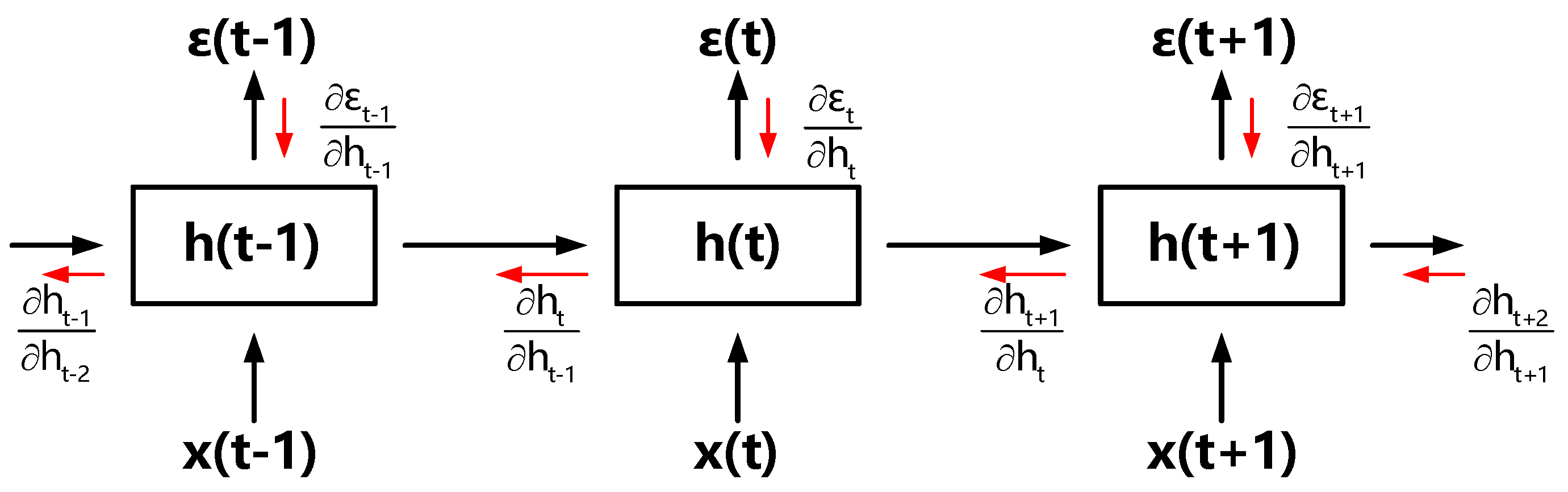
During RNNs training process, a stochastic gradient descent (SGD) algorithm is used with the theory of back-propagation through time (BPTT) [30], because of its recurrent temporal connections. The well-known BPTT algorithm is used to the calculate weight derivative for RNNs, with simple conception and efficient computation. It is simple to obtain the BPTT via unfolding RNNs in time, as shown in Figure 2.
The gradients are rewritten as a sum-of-products form in the timeline, in the light of [18],
where is the sum of temporal components, and indicates the effect of transmitting from the t-th time-step back to the k-th (is only suitable for forward-RNNs).
One can see that the gradient will vanish, i.e., if the constant , the norm of will go rapidly to 0 exponentially. Conversely, the gradient will explode to infinity, if . Note that it is unnecessary and impossible to keep at all time-steps, because the input series and the internal dynamics determine the activations of neurons in networks [31]. Faced with the correlated relationship in a long time-step span, the standard RNNs structure is awkward with regards to the gradient problem. There are some important branches of RNNs that appear to solve the long-term problem, such as LSTM [5,20,21] and Gated Recurrent Unit (GRU) [32] structures. However, these redesigned complex structures require specific training algorithms. Comparatively, we intend to attain a more concise structure with more general training methods, in order to achieve superb performance in various specific applications. For example, ECG signal classification using our proposed RNNs may have a promising performance in screening and preliminary diagnosis. Our reconstructed RNNs can analyze an infrared radiation intensity sequence of an object, in order to monitor changes in temperature. In addition, the method proposed in this paper can also be developed for image sequences or video classification, because of its excellent ability to learn correlations in information in the time domain.
3. Proposed BICORN-RNN
In this section, we formally propose an ingenious BIdirectional COnvolutional RaNdom RNN (BICORN-RNN) structure to solve the long-standing gradient problems in TSC processing.
A distinctive feature of BICORN-RNNs is an alternative combination of one or more improved measures. This sophisticated architecture has a probable contribution to discriminating different time series classes. From the different aspects and perspectives of input space, feature extraction, and transmission mode, different improvement methods are adopted correspondingly, and coordinate with each other. (1) The principal part of this novel model, RaNdom RNNs (RN-RNNs), is to project the classification prediction of previous time-steps into the current input, namely to modify the input space in order to easily catch important information; (2) There is a hierarchical part, COnvolutional RNNs (CO-RNNs), which extracts indescribable local features to enhance the ability of discrimination in different hierarchies, especially fine structures; (3) A symmetric part, BIdirectional transmission (BI-RNNs), provides access to the contexts on both sides of the series, so that it tends to gain a better performance because of its compensation for gradient problems.
3.1. Random Mapping Input Space
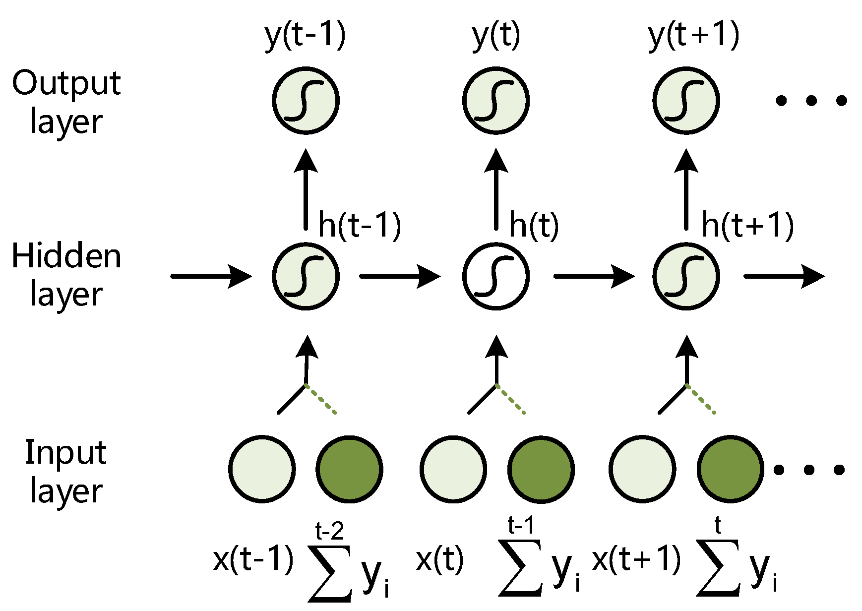
We assume that the network is built up properly, so as to obtain suitable dynamics dependencies. At each time-step, the network stores the previous outputs as an additional predictive sequence. We combine these predictions with the current input and feed it into the network, as illustrated in Figure 3.
This predictive information can provide more representative features and help extract more correlations within the input series. Note that the merger is in virtue of a saturating nonlinear function , such as logistic sigmoid function, squashing the two parts of the inputs into (0,1) nonlinearly, to avoid degeneration into a linear combination. So, at the t-th time-step, there is,
where x’(t) is the new input. It consists of two parts: one part is the original input value at the t-th time-step, that is x(t); the other part is the prediction information y(i) (i = 1,…, t-1) at each time before. And we use a random matrix to project y(i) onto a high-dimensional space , and then is weighted cumulative of . denotes the weight parameter which determines the proportion of the predicted output. We make to prevent immoderate predictions from vitiating or over-diluting x(t). Notably, a significant operation is random mapping, i.e., the previous predictions would be randomly projected onto a high-dimensional space by a random matrix , , whose elements are normally distributed in (0,1). It modifies the input data examples separately, and does not casually change the characteristics of the data itself. In addition, such non-linearity projections, akin to the kernel functions of support vector machines, have desirable properties in terms of nonlinear classification and regression problems.
Intuitively, random mapping can extend data from different labels to different directions, making the modified data more distinguishable. As the quasi-orthogonality property of a high-dimensional space proved in [33], when the dimension of the feature space T is relatively large, the column vectors of are much likely to be approximately orthogonal. It is a mathematical certainty that each column vector corresponds to the bias of per-class applied to the original sample x(t), if the real output y(t) is equal to the expected output . So, the random projection of previous predictions pushes the input examples apart from one another, with high probability [34].
The following proposition provides further evidence that, with accurate predictions of the target class in advance, it is possible to move the data manifolds apart by adding an offset to per-class examples, so as to guarantee an improvement in classification accuracy by using the RN-RNNs classifier.
Let be a set of data examples at the t-th time-step, where is the input example and is the target class label of x(t). Let be the corresponding parameters of RN-RNNs classifier with the loss function . Then, there exists such that the translated set defined as results in a better optimum .
Assume that f and g are the element-wise and monotonically increasing activation function and output function of the RN-RNNs classifier. Let be the row vector of in Equation (1). Defining such that , then we have,
where , refer to the element of the vector h(t), y(t) respectively. is the fixed term in Equation (1), regarded as a constant. In the TSC task, the loss function is often chosen as Cross-Entropy in Equation (8), and then,
which leads to .
It is important to note that learning the projection matrix may have a pure-perfect result in training sets, but not, regretfully, in testing sets, because of the overly confident strategy. On the premise of predictions y(t-m), in previous time-steps, learning-updating the elements of may suffer from over-fitting in all possibilities, which provided bad data or even a negative contribution in classification performance in the testing process. A conventional approach to avoid this is adding a regularization term in the loss function to constrain dynamic tuning. However, this would lead to additional parameters at each time-step, i.e., it will increase the computational complexity exponentially. Here, we might set the parameter matrix randomly without training, surprisingly, which is an agile and effective approach to solve both the overfitting and increasing computational complexity.
It is worth explaining that we aim to train an excellent generalization RNNs with the support of previous prediction information, rather than focusing on decorating data in a supervised way. Furthermore, this modification will not raise the dimension of the input space, and avoid the curse of dimensionality.
In fact, there is a large amount of computation in the training phase of RN-RNNs. The purpose of indexing from 1 to t − 1 is to force the retention of the information at earlier time-steps, highlighting its learning ability and reducing its dependency on long sequences. For more application scenarios, the sequence information at a very early time-step is often useless or redundant. Considering the limitation of computation and the demand of specific applications, we can modify Equation (10) to Equation (14) or Equation (15), as shown in following formulae:
Equation (10) indicates that the predictive information from the 1-th to (t-1)-th time-steps needs to be maintained and transmitted, to evoke the classification decision at the t-th time-step. However, the modified formulae have more pertinence in indexes with different meanings:
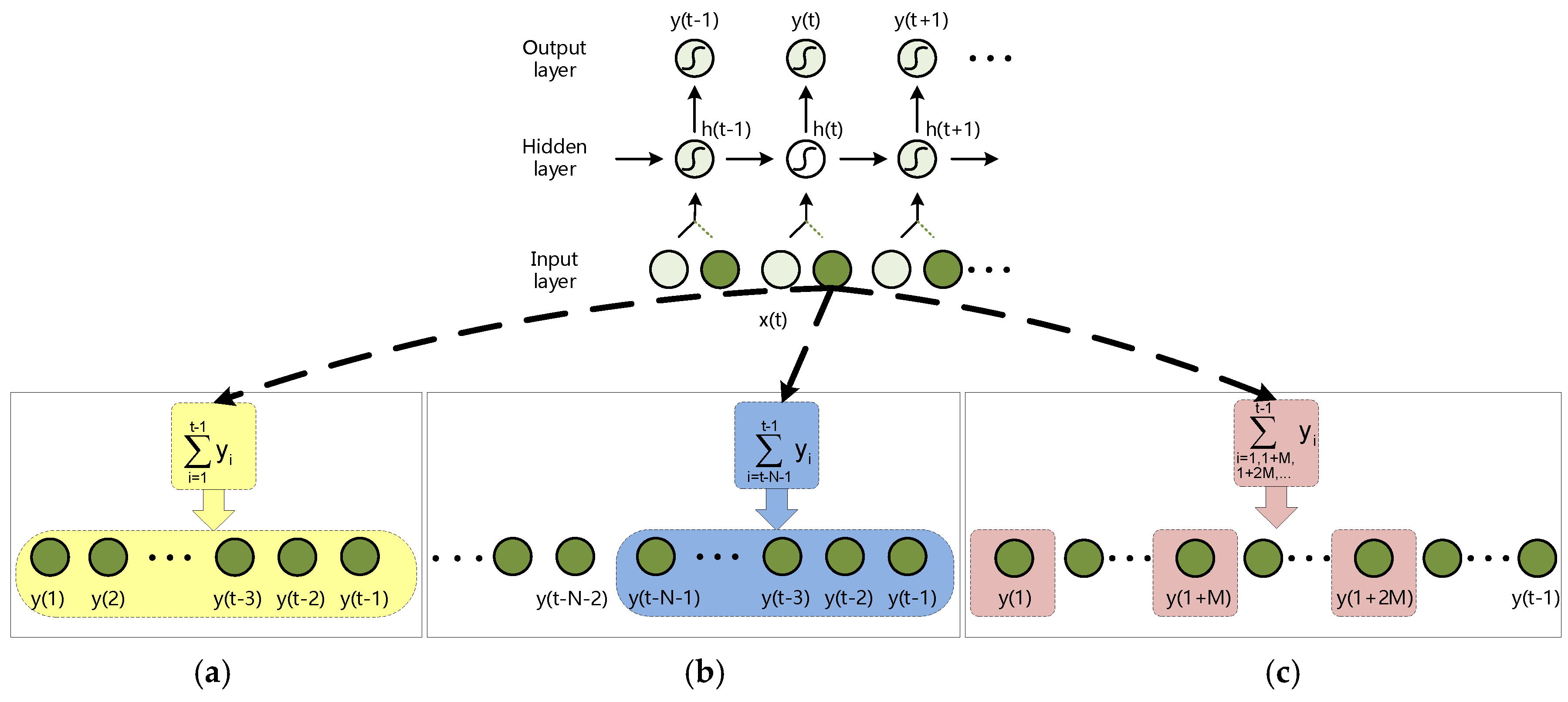
Equation (14) indicates that only the prediction values from the (t-N-1)-th to (t-1)-th time-steps, (N+1)-points sequence, are retained, because the value other than N-steps is too distant, its importance is greatly reduced, and it will not be involved in the classification decision at the t-th time-step. Equation (15) indicates that the prediction values from the 1-th to (t-1)-th time-steps are sampled at equal intervals M. Only these sample values are involved in the classification decision at the t-th time-step, which is more suitable for slowly changing and large time span sequences. The illustrations of the modified input values using different prediction information are shown in Figure 4.
These methods drastically reduce the amount of calculation, and they are also promising to maintain satisfying performance. The modification methods adopted in Equations (14) and (15) have more pertinence to the predictive output value. As shown in Figure 4b, Equation (14) focuses more on the key predictive values near the current moment, and ignores redundant old information. As shown in Figure 4c, Equation (15) samples all of the predictive output sequences ensure that the initial information can be transmitted effectively. Therefore, these two strategies for delivering predictive information have different advantages in specific application scenarios. Therefore, on the basis of appropriate input value x’(t), the network can gain a perfect temporal-dependencies learning capacity, and reduce the amount of computation. We compare the index times of these methods in Table 1.
This unsupervised random mapping is different from feature extraction, and the former can be regarded as the “separation” operation in the data preprocessing stage. Furthermore, unlike the overlapping technique, this improved method implies “prediction” information instead of a simple linear weighting combination of input points. The performance of the overlapping depends on an overlapping ratio, which is determined artificially. In contrast, the random mapping focuses on the predicted data to reduce the dependence on the quality of the input data virtually. In all, the aim of the random mapping is to solve the gradient vanishing and exploding problems in a concise way.
3.2. Convolutional Rearrange
Convolution can be regarded as a weighted superposition operation of one function upon another. The most typical application is convolution neural networks (CNNs) in deep learning, which has been successfully used in object recognition, audio classification, and image processing, because of key properties: spatially shared weights and spatial pooling [35].
RNNs pay more attention to the transmission of information between neurons at each time-step while ignoring the interconnection tendency of several points themselves, such as smoothness, volatility, periodicity, etc. Convolution is an ideal operation for extracting the indescribable local features of images, speech, and time series [36]. Therefore, it is not difficult to consider that an appropriate combination of convolution and RNNs, CO-RNNs, can enhance the ability to recollect and transmit the indispensable local features in online learning systems [37]. Actually, this “graft” can innovatively remove background noise and augment discrimination of data representations for classification tasks.
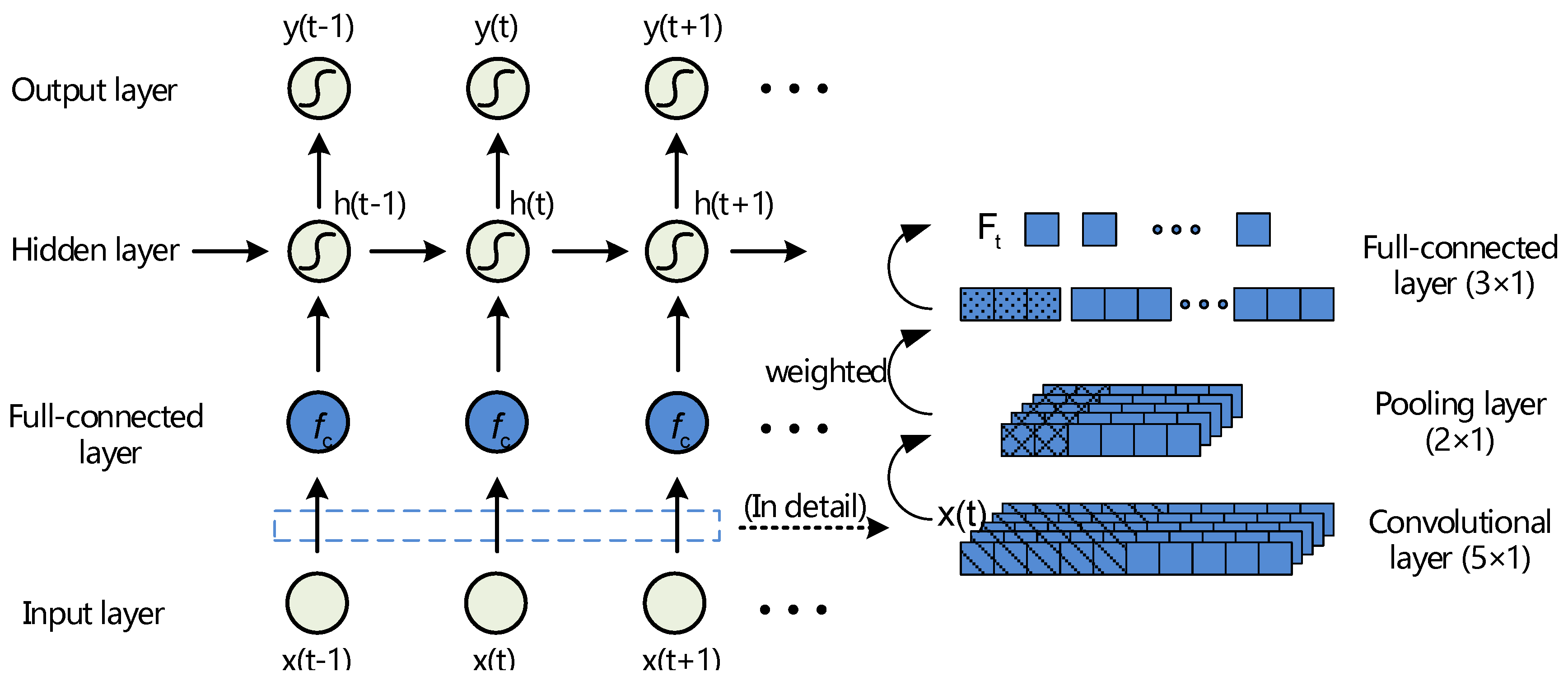
Specifically, we add a convolutional layer, a pooling layer, and a full-connected layer behind the input layer of RNNs, as shown in Figure 5. We do not recommend the convolutional operation behind the hidden layer, as it would disrupt the dynamic delivery of RNNs.
Concretely, similar to the common CNNs structure, the input example x(t) at the t-th time-step is convolved with learnable kernels () and put through a hyperbolic tangent function to form the output feature maps () of the convolutional layer. We use the average-pooling function to obtain the pooling feature maps (). Then, are projected onto the full-connected layer input maps (), by the linked weight . make convolutions with the full-connected kernel (), and are then activated by hyperbolic tangent function . Thus, the concatenation of each state () is finished, getting the new input series for CO-RNNs. The complete process is described as:
where “” denotes the convolutional operator, is the bias, represents a sub-sampling function. The fixed parameters are set by K-folder cross validation. The number of kernels and are set to 10 and 30 manually, and the size of plane is . Note that the random mapping described above is available and can coexist with convolutional rearranging operations in this subsection.
3.3. Bidirectional Transmission
The RNN is often considered to be a causal real-time system. Nevertheless, we can exploit anti-causal information of data to improve performance in non-immediate response issues, such as sentence translation and music style classification, which is the origin of bidirectional transmission of RNNs.
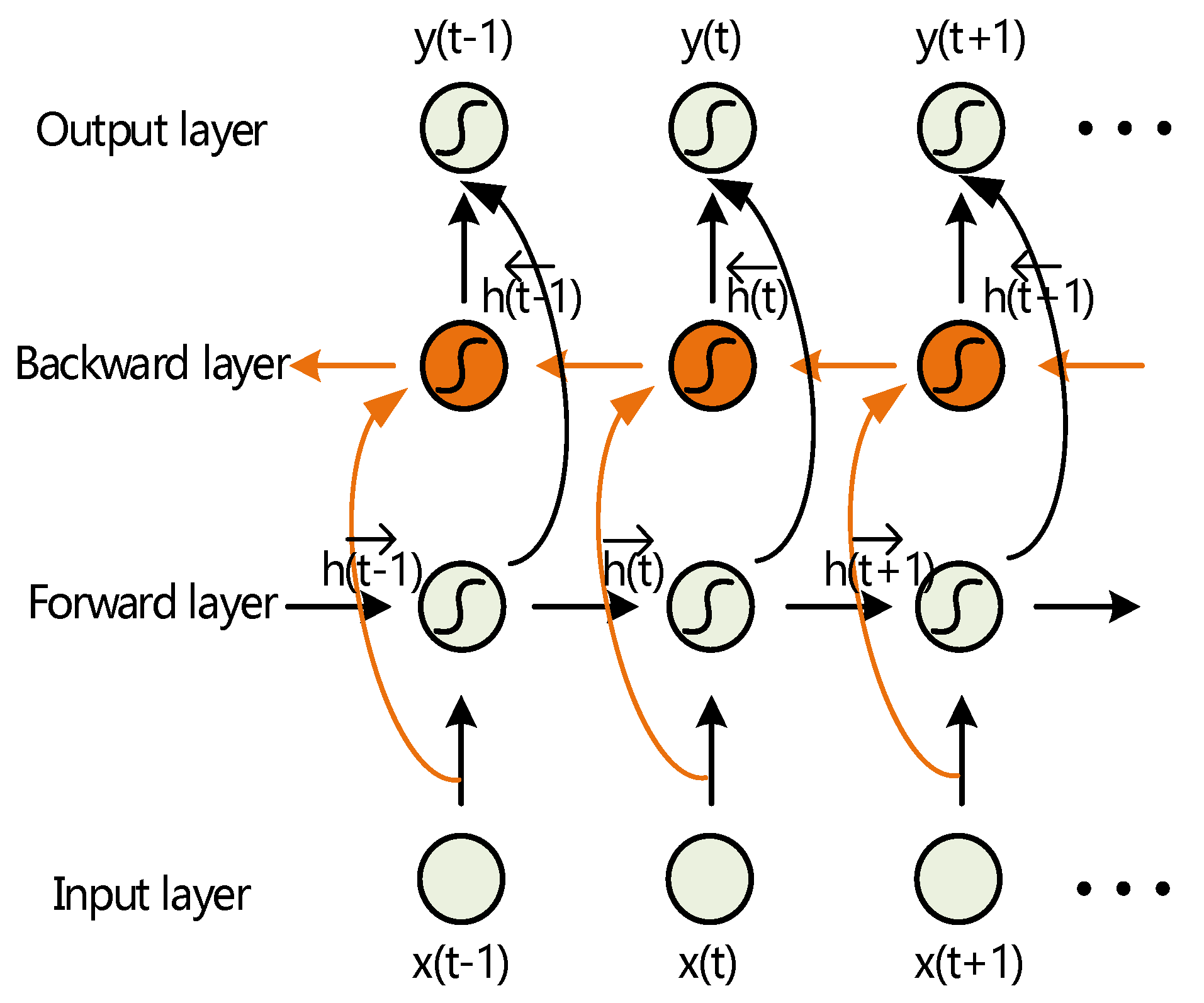
Bidirectional RNNs offer an elegant solution to make full use of both past and future data information in temporal order [38]. BI-RNNs transmit each point of a training sequence to both backward and forward two symmetry directions through by incorporating an extra hidden layer, called backward hidden layer, to distinguish from the original forward hidden layer.
Importantly, these two hidden layers are separated in space, so that they will not extend the parameter exponentially, but rather, will require twice the computation instead. We extend symbols by adding the arrows , , to the original representation, including variables and parameters, to refer to different transfer directions. So, the formulas of BIRNNs can be revised as,
We adjust weights and under the limitation of , to determine the importance of past and future information. Even without extra complex computations to train the networks, it is the same as SGD training algorithms of standard RNNs in Section 2. BI-RNNs can compensate for gradients vanishing and exploding problems by virtue of their own symmetry, as illustrated in Figure 6. Actually, BI-RNNs have outperformed standard RNNs in various previous applications, such as protein secondary structure prediction [39], speech processing [40], dynamic ECG analysis [41], as well as our TSC task.
3.4. BICORN-RNNs Structure
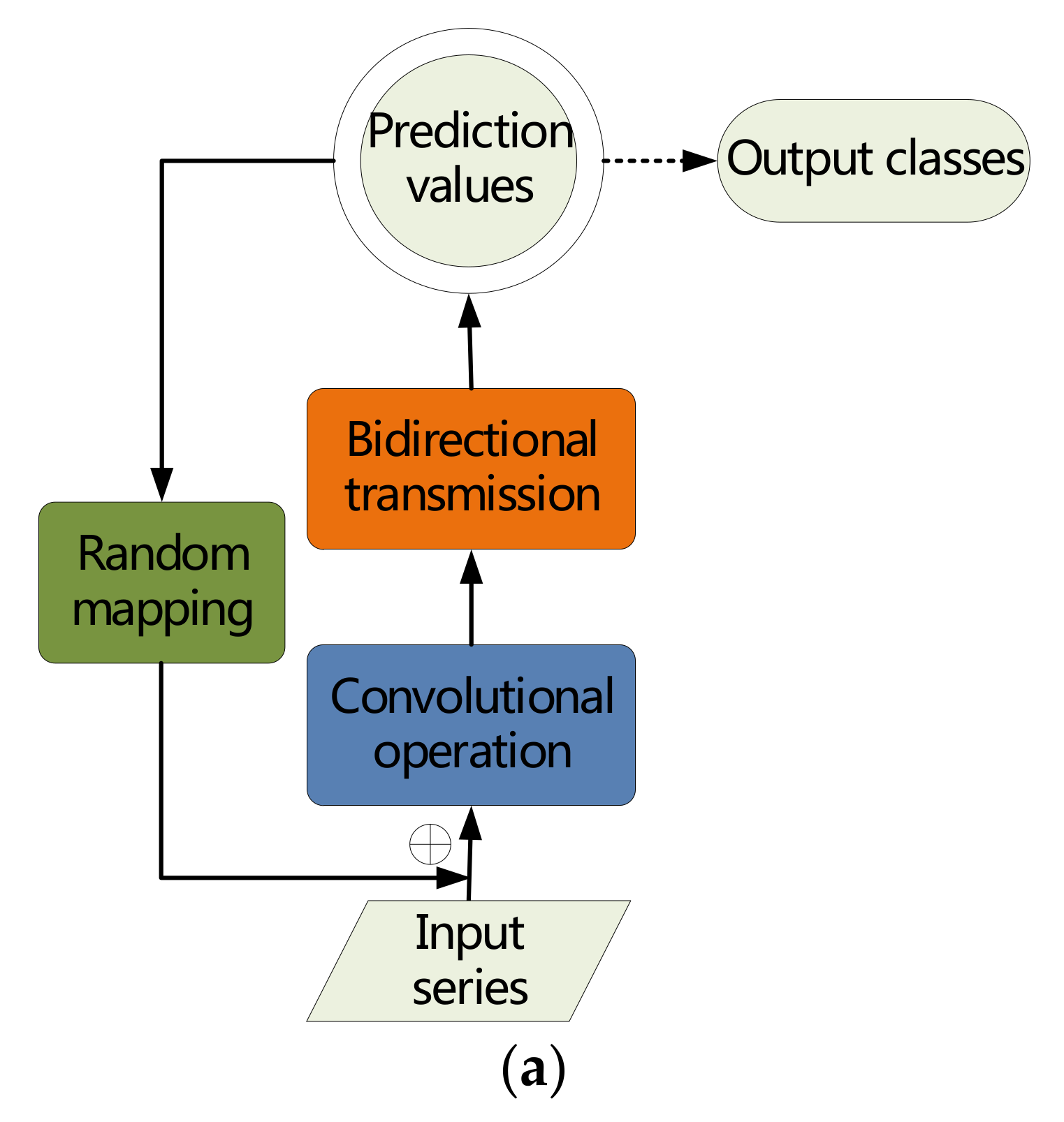
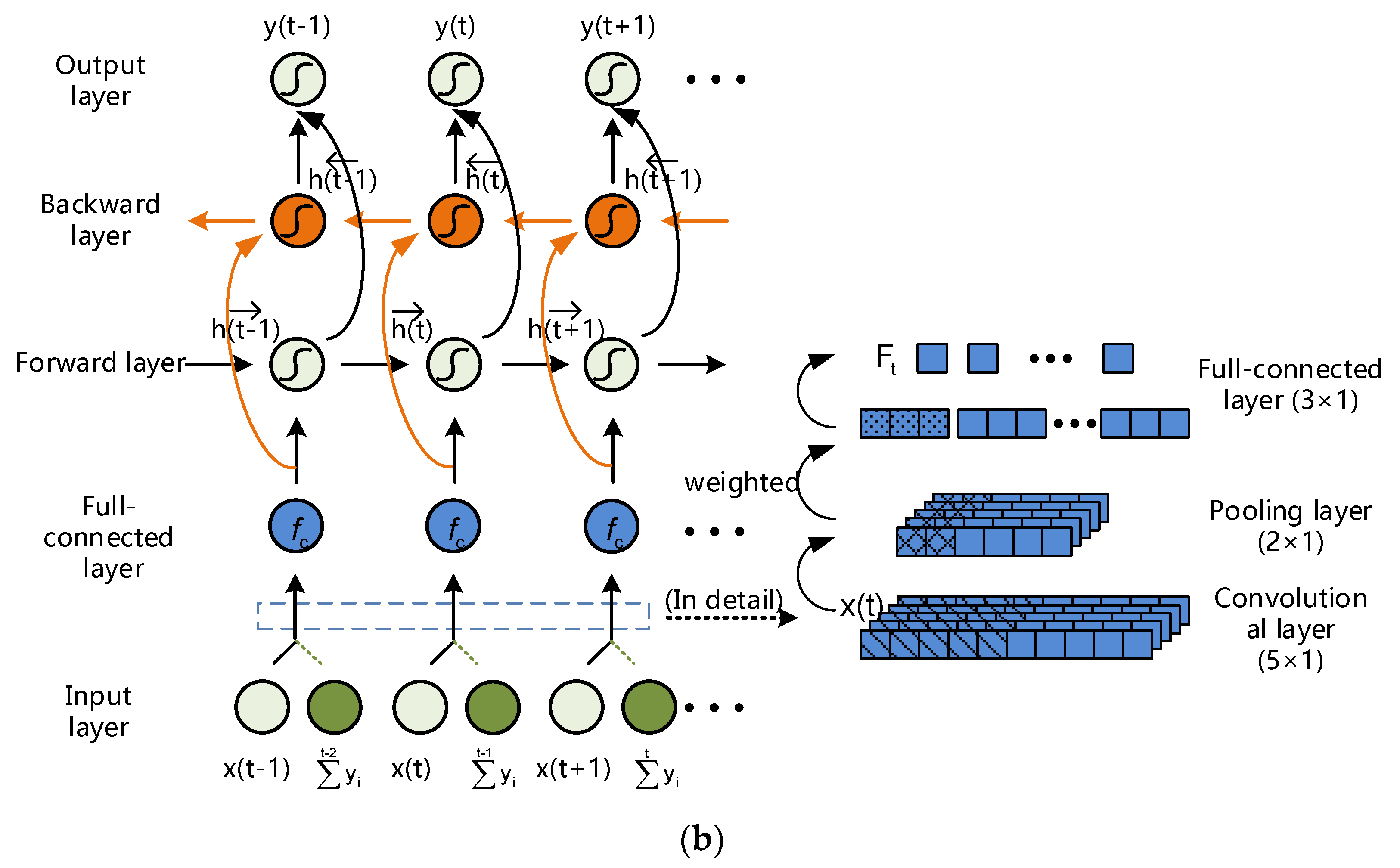
These modifications of basic RNNs architecture highlight the underlying characteristics of the data and the inherent structure of the model, which is crucial for improving classification performance. As shown in Figure 7a,b, we build an ever-improving RNNs structure, consisting of random mapping input space, convolutional rearranging, and bidirectional transmitting, namely BICORN-RNNs.
BICORN-RNN is not just a stack of a few improved methods; it redesigns network transmission processes from different angles and different levels to acquire a favorable structure. It should be emphasized that, although this full structure can obtain optimal performance under different conditions, we have access to the combination of one or more measures to construct a satisfactory structure, reflecting the flexibility of our method.
4. Experiments
In this section, we carry out experiments to compare the performance of multiple methods, and explore the influence of some factors on accuracy, in order to put up better choices of sub-model combinations.
4.1. Experiments on Benchmark Datasets
4.1.1. Experiments Description
We compare the performances of the introduced classifiers in Section 1 with 10 real-world datasets, selected from the UCR Time Series Classification Archive [42] randomly, which contains different application domains datasets, and is widely used as a benchmark for classification comparisons. To contrast with multiple types of classifiers, we have made an effort to consider some classical and effective methods, including (1) distance-based methods:1-NN with Euclidean distance (1NN-ED) [9] and 1-NN with DTW (1NN-DTW) [10], (2) feature-based methods: shapelets [11] and random forests based on features (Features-RF) [12], (3) ANN-based methods: feedforward neural networks (FNNs) [43], RNNs [17], LSTMs [20] and our BICORN-RNNs. It should be noted that the experimental results of type (1) and (2) were collected by [44,45], for an authoritative comparison. As for type (3), we use the default training and testing set splits provided by UCR for fairness concerning.
Without loss of generality, all neural network classifiers are set as a single layer hidden layer structure, and the number of neurons in hidden layer is 24. All weights in matrices are initialized in the interval drawn from the uniform distribution, where r and c are the number of rows and columns in the structure [46].
Generally, larger training sets can have a better generalization performance. However, considering the fact that it may suffer from the imbalanced percentages of training and testing examples in practical application, we improve the generalization performance with the limited datasets size through an early stopping method in the validation set, which avoids overfitting in the testing set. In this paper, both the validation error and training error are evaluated at regular intervals with a typical decrease. If the validation error appears to start increasing, the training will terminate at once.
4.1.2. Results and Discussion
We perform independent Monte-Carlo simulations under the preset parameters. We take the mean value of classification error rates as the final result to reduce accidental error. The classification error of each set is accurate to three decimal places, as shown in Table 2. It also shows the votes of the best results (Best), the first three results (Better-3) and the mean ranking (Mean-ranking) of each method for measurement.
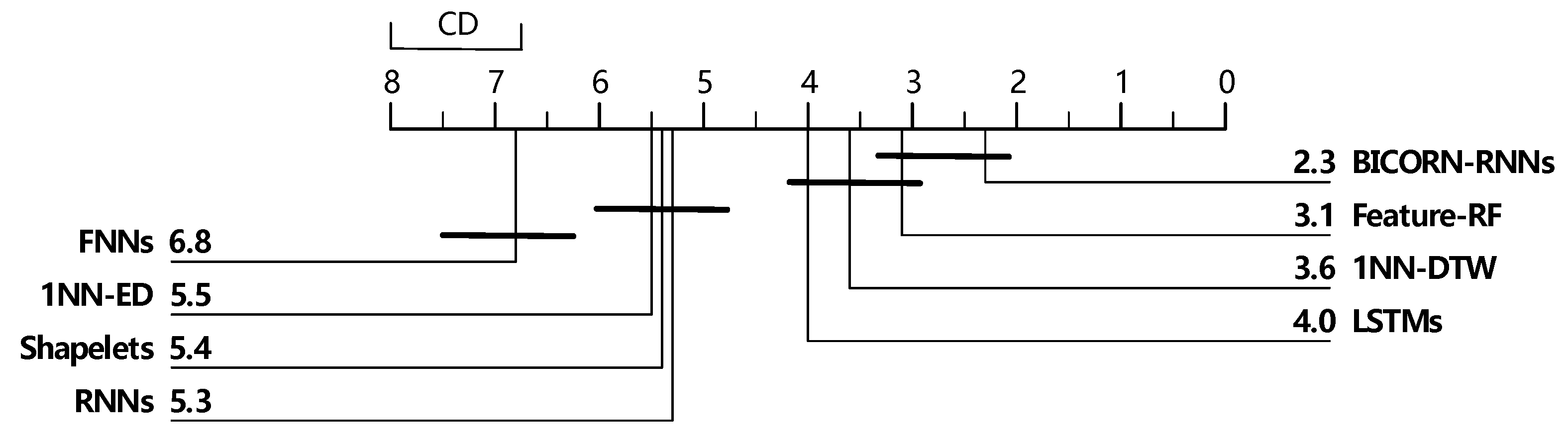
In addition to the intuitionistic judgment of the effectiveness of our method, we also illustrate the significant differences between our method and some other classical methods by the critical difference diagram (CDD), proposed in [47]. Figure 8 shows the CDD of eight methods above.
According to Figure 8, BICORN-RNNs obtain the highest accuracy, located in the furthest right of the figure; it is quite remarkable that this novel structure can effectuate such excellent classification performances in several datasets. We notice that the classification accuracies of FNNs and RNNs are the lowest, and they fail to gain assessments of “Best” or “Better-3”, whereas LSTMs, an improved branch of RNNs, demonstrate satisfactory performance. BICORN-RNNs gain a comprehensive victory in “Best”, “Better-3”, and “Mean-ranking”.
It is predictable that the rudimentary neural networks still fail to classify time series when faced with different characteristics. Fortunately, the fusion structure we proposed in this paper may have advantages in learning both data, and features, of the time series.
4.2. Experiments about Influencing Factors
4.2.1. Experiments Description
We have an appropriate data selection to facilitate cartographic analysis, for which the number of the classes should be , and the length of data time-steps should be . The assumption is to bring the fundamental setup of the experiments into this subsection, and ensure fairness among methods.
According to the criterion above, we use the dataset “OSU Leaf” to demonstrate the effectiveness of our approach. This shape-converted time series dataset is generated by radial scanning of the shape profile to convert the image into a one-dimension series. The dataset contains six classes, corresponding to six kinds of leaves with different shapes. Among them, the similarity between the first, second, third, and forth classes is high, and the similarity between the fifth, sixth classes is high [48].
The experiments follow the principle of controlling variables. We adjust several circumstances: the signal to noise ratio (SNR), truncated length, data missing, and overlapping. We train different RNNs-based classifiers with the same noise level; some of the basic experimental parameters settings are shown in Table 3.
4.2.2. Results regarding SNR and Discussion
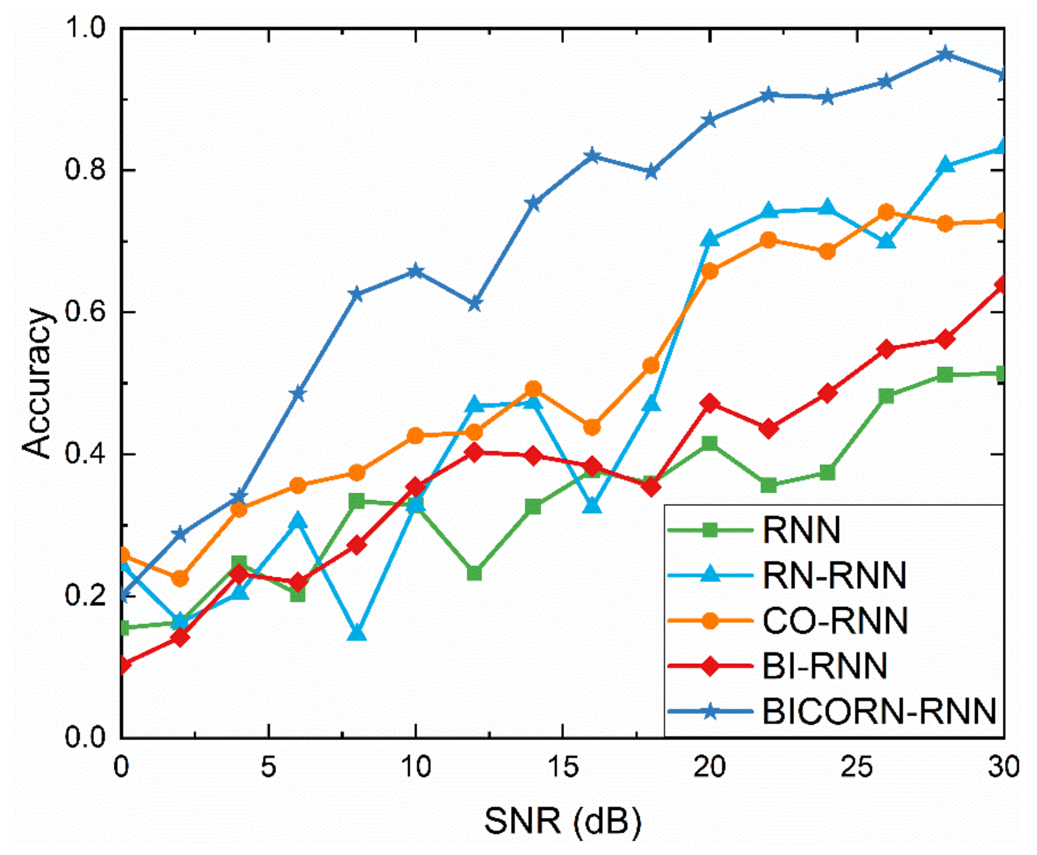
Noise disturbance is a problem often encountered in data analysis and processing. Therefore, this subsection aims to analyze the impact of noise (Gaussian noise) on the performance of the classifiers, and to verify the robustness of the proposed classifier at different SNR levels. We train different RNNs-based classifiers with the same noise level (20 dB), and test them with different noise levels (0 dB to 30 dB, stepped by 2 dB).
The classification results on the dataset “OSU Leaf” are shown in Figure 9. As shown in Figure 9, the classification accuracies of all methods are improved significantly with the increase in SNR, indicating that SNR is a key factor for TSC tasks. Additionally, BICORN-RNN maintains an obvious advantage when the SNR is greater than 5 dB, and it obtains more than 90% classification accuracy when the SNR is greater than 20 dB. As for 0 dB, the accuracies of all methods are around 20%. It is more inclined to classify data into 6 classes randomly because the signal is almost drowned out by noise.
Relatively, convolutional operation has a slight superiority over random mapping and bidirectional transmission, assuming a low SNR; this evidence shows that convolution is an effective method for filtering noise. Whereas random mapping might bring out more instability, i.e., it may exacerbate or counterbalance noise disturbances.
4.2.3. Results on Segmented Length and Discussion
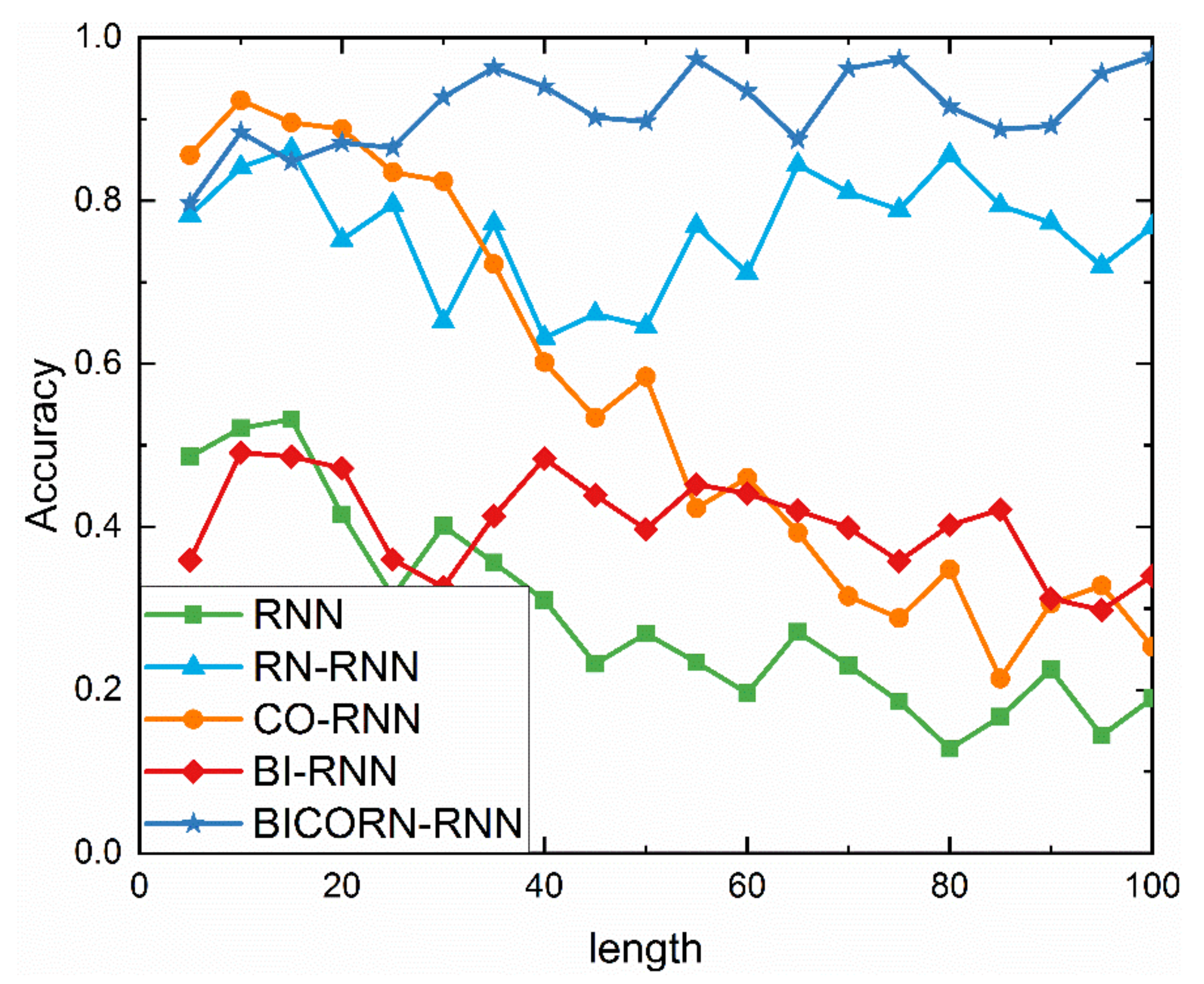
The variation of data length is a common phenomenon in time series analysis. This subsection aims to analyze the effect of data length on classification performance. We truncate time series into segments with different lengths (5 time-steps to 100 time-steps, stepped by 5 time-steps).
The classification results on the dataset “OSU Leaf” are shown in Figure 10. As seen in Figure 10, the sensitivity of these optimization methods to data length is definitely different. The accuracies of RN-RNN and BI-RNN do not fluctuate significantly with the increase in data length, which indicates that random mapping and bidirectional transmission can enhance long-term dependence to a greater or lesser degree.
Moreover, random mapping has more outstanding performance by remembering the previous predicted values compulsorily. Correspondingly, the convolutional operation lacks the direct temporal-dependency learning capability, especially in long time-steps, so the accuracy of CO-RNN declines more significantly.
However, as speculated from the results of RN-RNN and BICORN-RNN, the convolutional operation and bidirectional transmission help to improve the effect of random mapping indirectly, and only BICORN-RNN achieves a satisfactory classification accuracy of over 80%, regardless of the length of sequence. It also suggests that in some long time-step classification problems, we can try to remove the convolutional operation to simplify the networks, and still obtain adequate results.
4.2.4. Results regarding Data Missing and Discussion
Data missing refers to the loss of certain data (be set to 0) or the occurrence of large or small abnormal values. Data missing is usually in the absence of prior information; it is difficult to reproduce the data, so this problem is usually more lethal than Gaussian noise. There are some preprocesses methods to try to solve it, such as deleting defective cases and interpolating. For the former method, it is possible to lose valuable information and reduce samples; the latter introduces noise artificially. Other methods, such as robust regression, and high-dimensional mapping, are limited to complex calculations.
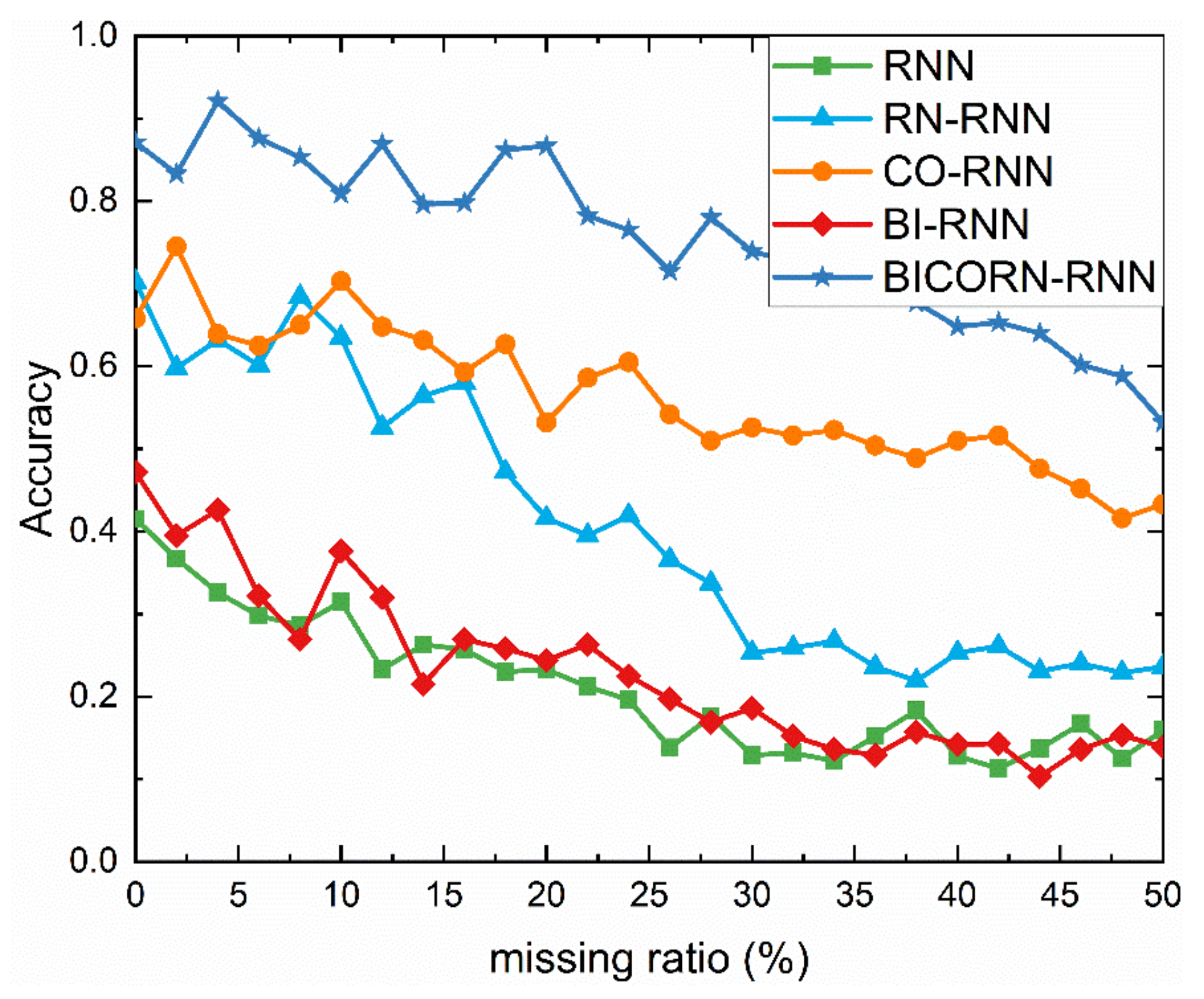
This subsection aims to demonstrate the robustness of our method without complicated preprocessing algorithm facing the data missing. We simulate different data missing ratio (0% to 50%, stepped by 5%), by setting an unusually large and small value at certain time-steps randomly.
The classification results on the dataset “OSU Leaf” are shown in Figure 11. As seen from Figure 11, facing the 50% data missing ratio, the accuracies of all classifiers have been significantly reduced by more than 20%. If the missing data ratio is less than 20%, the accuracy of BICORN-RNN can remain at over 80% with less fluctuation, which is the most robust one. It is reassuring that BICORN-RNN keeps a minimum accuracy line of 60% even if missing half of the data values, which may benefit from convolutional operation. By contrast, bidirectional transmission cannot be carried out smoothly whether forwards or backwards, due to the ineffective hidden values of the neurons during the processing; thus the accuracy of BI-RNN is attenuated as rapidly as that of the RNN, which is close to a random classification.
Although the integrity and validity of data is an important factor in maintaining high accuracy, the method we proposed can be efficacious provided that less than the half data is missing.
4.2.5. Result regarding Overlapping and Discussion
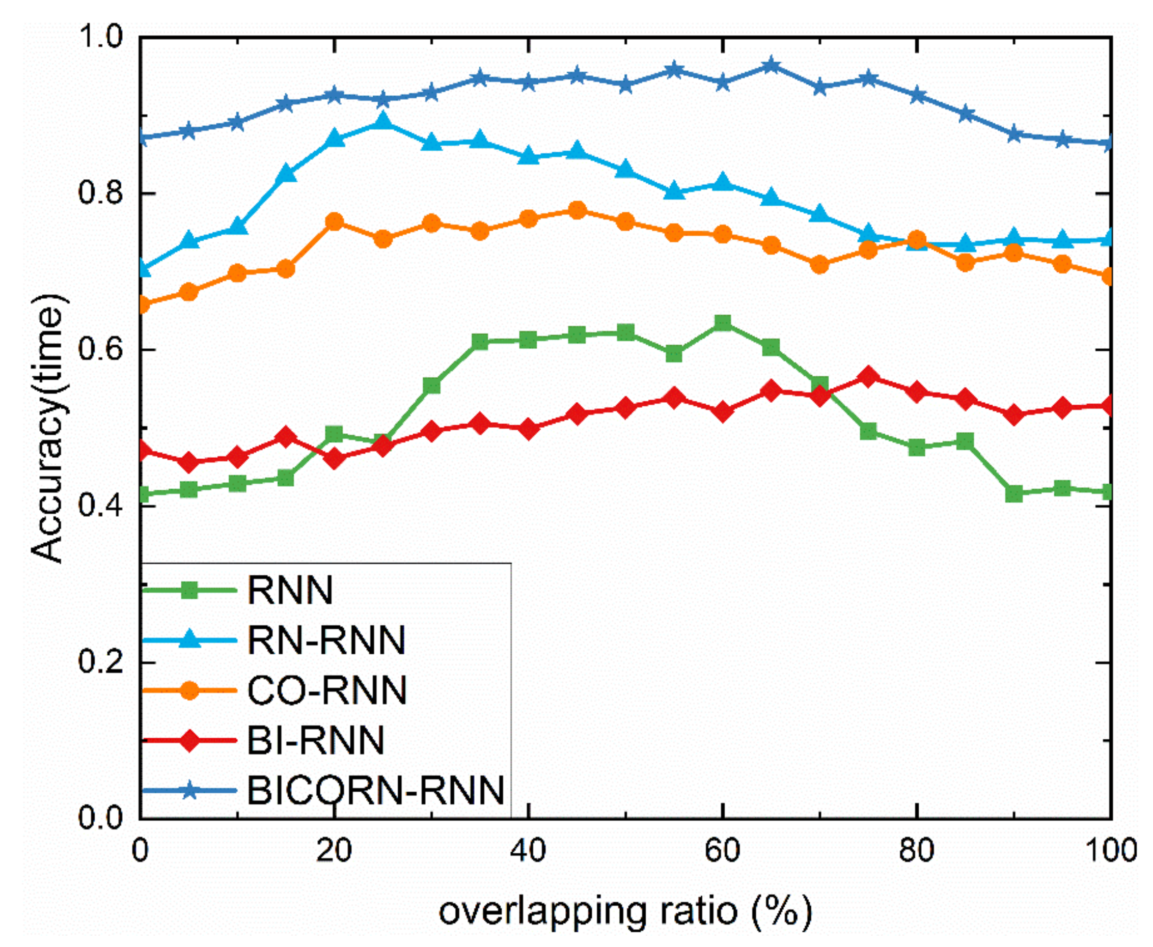
In Section 3, we deem that random mapping reduces the dependence on time-steps by forcing the memory of the previous prediction outputs, but it also weakens the information transmission ability of the hidden layer. This is why the classification accuracy of RN-RNN is more unstable than that of RNN when suffering from SNR variation, length change, or data missing, as shown in Figure 9, Figure 10 and Figure 11. However, we still believe that random mapping is an excellent solution to alleviate the problem of gradient vanishing and exploding, especially when reconsidering the potential information in hidden layer.
We use a simple and effective trick to improve the information transmission capability of RN-RNN in the hidden layer that is overlapping. It refers to the overlap between two adjacent input sequences, and aims to put more emphasis on the input data, which can be transmitted in the hidden layer further. Overlapping can improve the integrity of information with no prior information.
To analyze the information transmission capability in the hidden layer more clearly, we employ contrast experiments with vary accuracies in overlapping ratio, as shown in Figure 12. It is noteworthy that overlapping will inevitably increase the cost of computation. Both time and accuracy should be considered comprehensively, as timeliness is another important measure in our work.
A certain overlapping ratio of RNN and RN-RNN can improve the accuracy significantly, up to about 20% (the maximal accuracy of RN-RNN can be 90% with 25% overlapping ratio), while there is no prominent effect of overlapping in the other three methods: up to about 10% (the maximal accuracy of BICORN-RNN can be 95% with 65% overlapping ratio). However, it should not be overlooked that the extra calculation is obviously due to a high overlapping ratio. It also suggests that it would be beneficial to choose an RN-RNN with a precise overlapping ratio to ensure that a 90% accuracy is reached, while maintaining an acceptable real-time performance. The reason for the better accuracy of the RN-RNN is that overlapping compensates for the loss of information in hidden layer caused by random mapping.
4.3. Result about Synthetical Dataset and Discussion
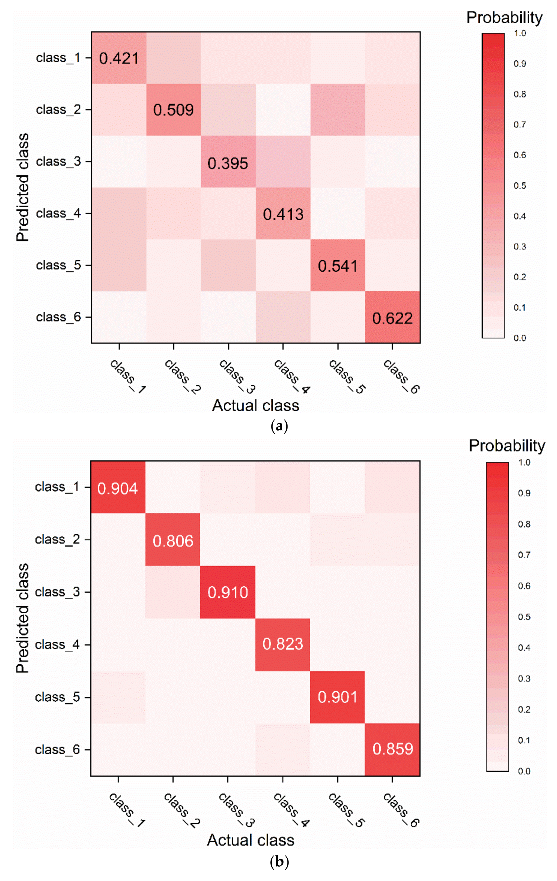
In Section 4 above, we generated 83 sets of experimental datasets “OSU Leaf” in total, including SNR (16 sets), segmented length (20 sets), data missing (26 sets), and overlapping (21 sets). Finally, RNN and BICORN-RNN methods are used to classify these time series in order to illustrate the effectiveness of our improved method.
The classification results of six classes are represented by the confusion matrices [49], as shown in Figure 13. The color block on the diagonal of matrix in Figure 13b is more concentrated than that in Figure 13a, indicating that the classification accuracy of BICORN-RNN in each class is higher than that of the RNN. Actually, the classification accuracy of BICORN-RNN is up to 86.72%, outperforming standard RNN, whose accuracy is 48.35%.
5. Conclusions
We have presented BIdirectional COnvolutional RaNdom RNNs (BICORN-RNNs), tailored for time series classification, based on the recurrent structure. It leverages the strength of RNNs in time to learn and classify sequences online. In addition, BICORN-RNNs have exceptional capabilities of information transmission based on gradient descent. Random mapping can remember the preceding information, and the local features of the time series can be extracted elaborately by a convolutional operation. As for bidirectional transmission, it provides convenient access to both future and past data, simultaneously. Above all, BICORN-RNNs incorporate the functions of these three independent measures; these measures can be integrated with each other flexibly and complementarily. We have demonstrated that BICORN-RNNs achieve fantastic performance via comprehensive experiments on public time series datasets, considering a variety of factors: SNR, length, data missing, and overlapping. It also suggests that these available sub-models can be chosen and combined to meet the needs of special tasks. Our work has a potential application in time series data analysis, such as natural language processing, biomedical diagnosis, audio classification and financial analysis. We envision that BICORN-RNNs will be extended in multiple sources, such as speech, text, and image sequences in scene classification domain.
Author Contributions
Ye Ma wrote the majority of the text and performed the design and implementation of the algorithm. Qing Chang and Huanzhang Lu commented on and approved the manuscript. Junliang Liu and contributed text to earlier versions of the manuscript and helped with the algorithm. All authors read and approved the final manuscript.
Conflicts of Interest
The authors declare no conflict of interest.
References
- Graves, A.; Beringer, N.; Schmidhuber, J. Rapid Retraining on Speech Data with LSTM Recurrent Networks; Technical Report; Instituto Dalle Molle di Studi Sull’ Intelligenza Artificiale: Manno, Switzerland, 2005. [Google Scholar]
- Mao, Y.; Chen, W.; Chen, Y.; Lu, C.; Kollef, M.; Bailey, T. An integrated data mining approach to real-time clinical monitoring and deterioration warning. In Proceedings of the 18th ACM SIGKDD International Conference on Knowledge Discovery and Data Mining, Beijing, China, 12–16 August 2012; pp. 1140–1148. [Google Scholar]
- Maharaj, E.A.; Alonso, A.M. Discriminant analysis of multivariate time series: Application to diagnosis based on ECG signals. Comput. Stat. Data Anal. 2014, 70, 67–87. [Google Scholar] [CrossRef]
- Daigo, K.; Tomoharu, N. Stock prediction using multiple time series of stock prices and news articles. In Proceedings of the 2012 IEEE Symposium on Computers & Informatics (ISCI), Penang, Malaysia, 18–20 March 2012; pp. 11–16. [Google Scholar]
- Karim, F.; Majumdar, S.; Darabi, H.; Chen, S. LSTM Fully Convolutional Networks for Time Series Classification. IEEE Access 2017, 6, 1662–1669. [Google Scholar] [CrossRef]
- Ding, H.; Trajcevski, G.; Scheuermann, P.; Wang, X.; Keogh, E. Querying and mining of time series data: Experimental comparison of representations and distance measures. Proc. Vldb Endow. 2008, 1, 1542–1552. [Google Scholar] [CrossRef]
- Wang, X.; Mueen, A.; Ding, H.; Trajcevski, G.; Scheuermann, P.; Keogh, E. Experimental comparison of representation methods and distance measures for time series data. Data Min. Knowl. Discov. 2013, 26, 275–309. [Google Scholar] [CrossRef]
- Oehmcke, S.; Zielinski, O.; Kramer, O. kNN ensembles with penalized DTW for multivariate time series imputation. In Proceedings of the 2016 International Joint Conference on Neural Networks, Vancouver, BC, Canada, 24–29 July 2016; pp. 2774–2781. [Google Scholar]
- Faloutsos, C.; Ranganathan, M.; Manolopoulos, Y. Fast subsequence matching in time-series databases. In Proceedings of the 1994 ACM SIGMOD International Conference on Management of Data, Minneapolis, MN, USA, 24–27 May 1994; pp. 419–429. [Google Scholar]
- Berndt, D.; Clihord, J. Using Dynamic Time Warping to Find Patterns in Sequences. In Proceedings of the 3rd International Conference on Knowledge Discovery and Data Mining, Seattle, WA, USA, 31 July–1 August 1994; pp. 359–370. [Google Scholar]
- Keogh, E.J.; Rakthanmanon, T. Fast Shapelets: A Scalable Algorithm for Discovering Time Series Shapelets. In Proceedings of the 2013 SIAM International Conference on Data Mining, Austin, TX, USA, 2–4 May 2013. [Google Scholar]
- Breiman, L. Random Forests. Mach. Learn. 2001, 45, 5–32. [Google Scholar] [CrossRef]
- Ye, L.; Keogh, E. Time Series Shapelets: A Novel Technique that Allows Accurate, Interpretable and Fast Classification. Data Min. Knowl. Discov. 2011, 22, 149–182. [Google Scholar] [CrossRef]
- Ye, L.; Keogh, E. Time series shapelets: A new primitive for data mining. In Proceedings of the ACM SIGKDD International Conference on Knowledge Discovery and Data Mining, Paris, France, 28 June–1 July 2009; pp. 947–956. [Google Scholar]
- Hinton, G.E. Learning multiple layers of representation. Trends Cogn. Sci. 2007, 11, 428–434. [Google Scholar] [CrossRef] [PubMed]
- WöHler, C.; Anlauf, J.K. An adaptable time-delay neural-network algorithm for image sequence analysis. IEEE Trans. Neural Netw. 1999, 10, 1531–1536. [Google Scholar] [CrossRef] [PubMed]
- Elman, J.L. Finding Structure in Time. Cogn. Sci. 1990, 14, 179–211. [Google Scholar] [CrossRef]
- Pascanu, R.; Mikolov, T.; Bengio, Y. On the difficulty of training recurrent neural networks. In Proceedings of the International Conference on International Conference on Machine Learning, Atlanta, GA, USA, 16–21 June 2013; pp. 1310–1318. [Google Scholar]
- Nair, V.; Hinton, G.E. Rectified linear units improve restricted boltzmann machines. In Proceedings of the International Conference on International Conference on Machine Learning, Haifa, Israel, 21–24 June 2010; pp. 807–814. [Google Scholar]
- Gers, F.A.; Schraudolph, N.N.; Schmidhuber, J. Learning precise timing with LSTM recurrent networks. J. Mach. Learn. Res. 2003, 3, 115–143. [Google Scholar]
- Mehdiyev, N.; Lahann, J.; Emrich, A.; Enke, D.; Fettke, P.; Loos, P. Time Series Classification using Deep Learning for Process Planning: A Case from the Process Industry. Procedia Comput. Sci. 2017, 114, 242–249. [Google Scholar] [CrossRef]
- Achanta, S.; Alluri, K.R.; Gangashetty, S.V. Statistical Parametric Speech Synthesis Using Bottleneck Representation from Sequence Auto-encoder. arXiv, 2016; arXiv:1606.05844. [Google Scholar]
- Bengio, Y.; Simard, P.; Frasconi, P. Learning long-term dependencies with gradient descent is difficult. IEEE Trans. Neural Netw. 2002, 5, 157–166. [Google Scholar] [CrossRef] [PubMed]
- Islam, M.M.; Sattar, M.A.; Amin, M.F.; Murase, K. A New Adaptive Strategy for Pruning and Adding Hidden Neurons during Training Artificial Neural Networks. In International Conference on Intelligent Data Engineering and Automated Learning; Springer: Berlin/Heidelberg, Germany, 2008; pp. 40–48. [Google Scholar]
- Panchal, G.; Ganatra, A.; Kosta, Y.P.; Panchal, D. Behaviour analysis of multilayer perceptrons with multiple hidden neurons and hidden layers. Int. J. Comput. Theory Eng. 2011, 3, 332–337. [Google Scholar] [CrossRef]
- Shore, J.E.; Johnson, R.W. Properties of cross-entropy minimization. IEEE Trans. Inf. Theory 1981, 27, 472–482. [Google Scholar] [CrossRef]
- Bridle, J.S. Probabilistic Interpretation of Feedforward Classification Network Outputs, with Relationships to Statistical Pattern Recognition. In Neurocomputing; Springer: Berlin/Heidelberg, Germany, 1990; pp. 227–236. [Google Scholar]
- Martens, J.; Sutskever, I. Learning recurrent neural networks with hessian-free optimization. In Proceedings of the International Conference on International Conference on Machine Learning, Bellevue, WA, USA, 28 June–2 July 2011; pp. 1033–1040. [Google Scholar]
- Zhang, N.; Behera, P.K. Solar radiation prediction based on recurrent neural networks trained by Levenberg-Marquardt backpropagation learning algorithm. In Proceedings of the IEEE PES Innovative Smart Grid Technologies, Washington, DC, USA, 16–20 January 2012; IEEE Computer Society: Washington, DC, USA, 2012; pp. 1–7. [Google Scholar]
- Rumelhart, D.; Mcclelland, J. Learning Internal Representations by Error Propagation. In Neurocomputing: Foundations of Research; MIT Press: Cambridge, MA, USA, 1988; pp. 318–362. [Google Scholar]
- Hüsken, M.; Stagge, P. Recurrent neural networks for time series classification. Neurocomputing 2003, 50, 223–235. [Google Scholar] [CrossRef]
- Chung, J.; Gulcehre, C.; Cho, K.; Bengio, Y. Empirical Evaluation of Gated Recurrent Neural Networks on Sequence Modeling. arxiv, 2014; arXiv:1412.3555. [Google Scholar]
- Vesanto, J.; Alhoniemi, E. Clustering of the self-organizing map. IEEE Trans. Neural Netw. 2000, 11, 586–600. [Google Scholar] [CrossRef] [PubMed]
- Vinyals, O.; Jia, Y.; Deng, L.; Darrell, T. Learning with recursive perceptual representations. In Proceedings of the Advances in Neural Information Processing Systems 25 (NIPS), Lake Tahoe, NV, USA, 3–6 December 2012. [Google Scholar]
- He, K.; Zhang, X.; Ren, S.; Sun, J. Spatial Pyramid Pooling in Deep Convolutional Networks for Visual Recognition. IEEE Trans. Pattern Anal. Mach. Intell. 2014, 37, 1904–1916. [Google Scholar] [CrossRef] [PubMed]
- Lecun, Y.; Bengio, Y. Convolutional networks for images, speech, and time series. In The Handbook of Brain Theory and Neural Networks; MIT Press: Cambridge, MA, USA, 1998. [Google Scholar]
- Lin, S.; Runger, G.C. GCRNN: Group-Constrained Convolutional Recurrent Neural Network. IEEE Trans. Neural Netw. Learn. Syst. 2017, 1–10. [Google Scholar] [CrossRef]
- Schuster, M.; Paliwal, K.K. Bidirectional recurrent neural networks. IEEE Trans. Signal Process. 1997, 45, 2673–2681. [Google Scholar] [CrossRef]
- Baldi, P.; Brunak, S.; Frasconi, P.; Pollastri, G.; Soda, G. Bidirectional Dynamics for Protein Secondary Structure Prediction. Seq. Learn. Paradig. Algorithms Appl. 2000, 21, 99–120. [Google Scholar]
- Schuster, M. On Supervised Learning from Sequential Data with Applications for Speech Recognition. Ph.D. Thesis, Nara Institute of Science and Technology, Ikoma, Japan, 15 February 1999. [Google Scholar]
- Ibeyli, E.D. Recurrent neural networks employing Lyapunov exponents for analysis of ECG signals. Expert Syst. Appl. 2010, 37, 1192–1199. [Google Scholar]
- Chen, Y.; Keogh, E.; Hu, B.; Begum, N.; Bagnall, A.; Mueen, A.; Batista, G. The UCR Time Series Classification Archive. 2015. Available online: www.cs.ucr.edu/~eamonn/time_series_data/ (accessed on 18 April 2015).
- Chen, K.; Kvasnicka, V.; Kanen, P.C.; Haykin, S. Feedforward Neural Network Methodology. IEEE Trans. Neural Netw. 2001, 12, 647–648. [Google Scholar] [CrossRef]
- Bagnall, A.; Lines, J.; Hills, J.; Bostrom, A. Time-Series Classification with COTE: The Collective of Transformation-Based Ensembles. IEEE Trans. Knowl. Data Eng. 2015, 27, 2522–2535. [Google Scholar] [CrossRef]
- Schafer, P. Scalable time series classification. Data Min. Knowl. Discov. 2016, 30, 1273–1298. [Google Scholar] [CrossRef]
- Glorot, X.; Bengio, Y. Understanding the difficulty of training deep feedforward neural networks. In Proceedings of the International Conference on Artificial Intelligence and Statistics, Sardinia, Italy, 13–15 May 2010; pp. 249–256. [Google Scholar]
- Demsar, J. Statistical Comparisons of Classifiers over Multiple Data Sets. J. Mach. Learn. Res. 2006, 7, 1–30. [Google Scholar]
- Gandhi, A. Content-based Image Retrieval: Plant Species Identification. Master’s Thesis, Oregon State University, Corvallis, OR, USA, 2011. [Google Scholar]
- Landgrebe, T.C.W.; Duin, R.P.W. Efficient Multiclass ROC Approximation by Decomposition via Confusion Matrix Perturbation Analysis. IEEE Trans. Pattern Anal. Mach. Intell. 2008, 30, 810–822. [Google Scholar] [CrossRef] [PubMed]
Figure 1.
Unfolding a recurrent neural network structure proposed by Elman (Elman-RNNs) in time by creating a copy of the model at each time-step; arrows indicate the flow of information inside the network.
Figure 1.
Unfolding a recurrent neural network structure proposed by Elman (Elman-RNNs) in time by creating a copy of the model at each time-step; arrows indicate the flow of information inside the network.

Figure 2.
Deriving the gradients according to the back-propagation through time (BPTT) method. We denote by the error obtained from the output at the t-th time-step.
Figure 2.
Deriving the gradients according to the back-propagation through time (BPTT) method. We denote by the error obtained from the output at the t-th time-step.

Figure 3.
Illustration of an unfolded (RaNdom Recurrent Neural Networks) RN-RNN in time, where the input receives the random projection of output predictions of all the previous time-steps.
Figure 3.
Illustration of an unfolded (RaNdom Recurrent Neural Networks) RN-RNN in time, where the input receives the random projection of output predictions of all the previous time-steps.

Figure 4.
Illustration of the modified input values using different prediction information described in Equations (10), (14) and (15): (a) Index from the 1-th to (t-1)-th time-steps, corresponding to Equation (10); (b) Index from the (t-N-1)-th to (t-1)-th time-steps, corresponding to Equation (14); (c) Index from the 1-th to (t-1)-th time-steps, and sampling at equal intervals M, corresponding to Equation (15).

Figure 5.
Illustration of COnvolutional Recurrent Neural Networks (CN-RNNs) architecture and the procedures of convolution and pooling operations.
Figure 5.
Illustration of COnvolutional Recurrent Neural Networks (CN-RNNs) architecture and the procedures of convolution and pooling operations.

Figure 6.
An unfolded BIdirectional Recurrent Neural Networks (BI-RNNs) in time, in which no information flows between opposite direction layers, to ensure the acyclicity of unfolded units.
Figure 6.
An unfolded BIdirectional Recurrent Neural Networks (BI-RNNs) in time, in which no information flows between opposite direction layers, to ensure the acyclicity of unfolded units.

Figure 7.
Overall architecture of BIdirectional COnvolutional RaNdom Recurrent Neural Networks (BICORN-RNNs): (a) The complete process of BICORN-RNNs; (b) The main architecture of our neural network and the detail of the sub-models.
Figure 7.
Overall architecture of BIdirectional COnvolutional RaNdom Recurrent Neural Networks (BICORN-RNNs): (a) The complete process of BICORN-RNNs; (b) The main architecture of our neural network and the detail of the sub-models.


Figure 8.
Critical difference diagram over mean ranks of 8 methods belonging to 3 categories. Each label corresponds to the mean ranking of each classifier; the smaller the value, the better performance of the method. The length of bold lines indicates the critical difference with a confidence level of 0.05, which means that a group of classifiers with a bold line shows no significant difference. The critical difference is 1.25. Our classifier was the most optimal in all eight methods.

Figure 9.
Comparison of several improved classifiers, including the full structure BICORN-RNN, to standard RNN with different SNR.
Figure 9.
Comparison of several improved classifiers, including the full structure BICORN-RNN, to standard RNN with different SNR.

Figure 10.
Comparison of several improved classifiers, including the full structure BICORN-RNN, with standard RNN with different lengths of sequences.
Figure 10.
Comparison of several improved classifiers, including the full structure BICORN-RNN, with standard RNN with different lengths of sequences.

Figure 11.
Comparison of several improved classifiers, including the full structure BICORN-RNN, to standard RNN with different missing data ratios.
Figure 11.
Comparison of several improved classifiers, including the full structure BICORN-RNN, to standard RNN with different missing data ratios.

Figure 12.
Comparison of several improved classifiers, including the full structure BICORN-RNN, to standard RNN with different overlapping ratio.
Figure 12.
Comparison of several improved classifiers, including the full structure BICORN-RNN, to standard RNN with different overlapping ratio.

Figure 13.
On the right side of each figure, the color depth corresponds to accuracy; the deeper the color, the higher the accuracy. The confusion matrices show the correspondence between the predicted and the actual classes. Only the results on diagonal lines are correct. The values in the confusion matrices indicate the classification accuracy of each class. (a) Classification result of RNN; (b) Classification result of BICORN-RNN.


Table 1.
The index times of three methods with different criteria.
| Methods | 1~(t-1) time-steps | (t-N-1)~(t-1) time-steps | 1~(t-1) time-steps (sampled at M) |
|---|---|---|---|
| Times of indexes |
Table 2.
Classification error and performance ranking. The values in parentheses indicate the performance ranks of the different methods in three categories, and the optimal result of each dataset is represented as a bold number.
Table 2.
Classification error and performance ranking. The values in parentheses indicate the performance ranks of the different methods in three categories, and the optimal result of each dataset is represented as a bold number.
| Dataset | Distance-Based | Feature-Based | ANN-Based | |||||
|---|---|---|---|---|---|---|---|---|
| 1NN-ED | 1NN-DTW | Shapelets | Features-RF | FNNs | RNNs | LSTM | BICORN-RNNs | |
| 50Words | 0.369(3) | 0.310(1) | 0.489(6) | 0.333(2) | 0.677(8) | 0.641(7) | 0.425(5) | 0.408(4) |
| ChlorineCon | 0.352(7) | 0.350(6) | 0.417(8) | 0.272(5) | 0.209(3) | 0.174(2) | 0.213(4) | 0.165(1) |
| ECG | 0.232(8) | 0.203(7) | 0.004(1) | 0.158(5) | 0.160(6) | 0.146(4) | 0.120(3) | 0.097(2) |
| Fish | 0.217(6) | 0.177(3) | 0.197(4) | 0.157(2) | 0.302(8) | 0.253(7) | 0.208(5) | 0.154(1) |
| MoteStrain | 0.121(4) | 0.165(5) | 0.217(8) | 0.103(2) | 0.194(7) | 0.188(6) | 0.101(1) | 0.114(3) |
| OliveOil | 0.133(3) | 0.167(5) | 0.213(7) | 0.093(1) | 0.302(8) | 0.150(4) | 0.211(6) | 0.102(2) |
| Lightning7 | 0.425(6) | 0.274(1) | 0.403(4) | 0.295(2) | 0.552(8) | 0.545(7) | 0.386(3) | 0.412(5) |
| SwedishLeaf | 0.213(5) | 0.208(4) | 0.269(8) | 0.088(2) | 0.259(7) | 0.248(6) | 0.103(3) | 0.087(1) |
| Symbols | 0.100(7) | 0.050(3) | 0.068(4) | 0.138(8) | 0.091(6) | 0.083(5) | 0.042(2) | 0.023(1) |
| SyntheticControl | 0.120(6) | 0.007(1) | 0.081(4) | 0.017(2) | 0.139(7) | 0.097(5) | 0.156(8) | 0.024(3) |
| Best | 0 | 3 | 1 | 1 | 0 | 0 | 1 | 4 |
| Better-3 | 2 | 5 | 1 | 7 | 1 | 1 | 5 | 8 |
| Mean-ranking | 5.5 | 3.6 | 5.4 | 3.1 | 6.8 | 5.3 | 4.0 | 2.3 |
1NN-ED: 1-nearest neighbor with Euclidean distance; 1NN-DTW: 1-nearest neighbor with dynamic time warping; RF: random forests based on features; ANN: artificial neural network; FNNs: feedforward neural networks; RNNs: recurrent neural networks; LSTM: long-short time memory.
Table 3.
A summary of the experimental basic setup.
| Experiments | SNR (dB) | Length (Time-Steps) | Missing Ratio (%) | Overlapping Ratio (%) |
|---|---|---|---|---|
| 4.2.2 | Range: 0~30 Step: 2 | 20 | 0 | 0 |
| 4.2.3 | 20 | Range: 5~100 Step: 5 | 0 | 0 |
| 4.2.4 | 20 | 20 | Range: 0~50 Step: 2 | 0 |
| 4.2.5 | 20 | 20 | 0 | Range: 0~100 Step: 5 |
SNR: signal-to-noise ratio, is defined as the ratio of signal power to the noise power.
© 2018 by the authors. Licensee MDPI, Basel, Switzerland. This article is an open access article distributed under the terms and conditions of the Creative Commons Attribution (CC BY) license (http://creativecommons.org/licenses/by/4.0/).
Share and Cite
MDPI and ACS Style
Ma, Y.; Chang, Q.; Lu, H.; Liu, J. Reconstruct Recurrent Neural Networks via Flexible Sub-Models for Time Series Classification. Appl. Sci. 2018, 8, 630. https://0-doi-org.brum.beds.ac.uk/10.3390/app8040630
AMA Style
Ma Y, Chang Q, Lu H, Liu J. Reconstruct Recurrent Neural Networks via Flexible Sub-Models for Time Series Classification. Applied Sciences. 2018; 8(4):630. https://0-doi-org.brum.beds.ac.uk/10.3390/app8040630
Chicago/Turabian StyleMa, Ye, Qing Chang, Huanzhang Lu, and Junliang Liu. 2018. "Reconstruct Recurrent Neural Networks via Flexible Sub-Models for Time Series Classification" Applied Sciences 8, no. 4: 630. https://0-doi-org.brum.beds.ac.uk/10.3390/app8040630
Note that from the first issue of 2016, this journal uses article numbers instead of page numbers. See further details here.