A Novel Swarm Optimisation Algorithm Based on a Mixed-Distribution Model

Abstract

Many swarm intelligence optimisation algorithms have been inspired by the collective behaviour of natural and artificial, decentralised, self-organised systems. Swarm intelligence optimisation algorithms have unique advantages in solving certain complex problems that cannot be easily solved by traditional optimisation algorithms. Inspired by the adaptive phenomena of plants, a novel evolutionary algorithm named the bean optimisation algorithm (BOA) is proposed, which combines natural evolutionary tactics and limited random searches. It demonstrates stable behaviour in experiments and is a promising alternative to existing optimisation methods for engineering applications. A novel distribution model for BOA is built through research and study on the relevant research results of biostatistics. This model is based on a combination of the negative binomial and normal distributions, and the resulting algorithm is called NBOA. To validate NBOA, function optimisation experiments are carried out, which include ten typical benchmark functions. The results indicate that NBOA performs better than particle swarm optimisation (PSO) and BOA. We also investigate the characteristics of NBOA and conduct a contrast analysis to verify our conclusions about the relationship between its parameters and its performance.

1. Introduction

Swarm intelligence was first proposed by Gerardo Beni and Jing Wang of the University of California in 1989. It was used in cell robots, and focuses on the behaviour and control of groups based on bio-intelligence theory and methods [1]. In the early 1990s, swarm intelligence algorithms were proposed that simulate the cooperative behaviour of groups of social animals. The core concept of swarm intelligence is that swarms composed of simple individuals can achieve more complex functions simply by cooperating with each other. Therefore, it is possible to solve complex distributed problems using swarm intelligence, which works on the premise of there being no centralised control and no global information or models.

Unlike the classical optimization algorithm using deterministic rules, the swarm intelligence algorithm lets individuals search in the solution space simultaneously by using the probability transfer mode and a variety of random factors combined with metaheuristic rules. Research has produced increasing numbers of swarm intelligence algorithms, such as particle swarm optimisation (PSO) [2], ant colony optimisation (ACO) [3], the artificial fish-swarm algorithm [4], the free search algorithm [5], the human evolution model algorithm [6], the group search optimisation algorithm [7], the bees algorithm [8], bacterial foraging optimisation [9], the shuffled frog leaping algorithm [10], the fireworks algorithm [11], information feedback models [12], evolutionary multi-objective optimization algorithms [13], the krill herd algorithm [14,15], the harmony search algorithm [16], monarch butterfly optimization [17], the moth search algorithm [18], and cuckoo search [19]. Because biological structures are sophisticated, they have high degrees of adaptive capacity and strong collaborative capabilities, both in terms of evolution and behaviour [20]. The swarm intelligence algorithm is generally coordinated by a group of individuals (social insects, or particles). It has the ability to communicate (directly or indirectly) and interactively adapt to the environment so that the individual’s adaptability to the environment becomes better and better, and a good approximate solution is gradually obtained for the global optimal solution to the problem. Presently, because of its high scalability and flexibility, researchers have applied swarm intelligence algorithm to many areas, such as scheduling [21], parameter estimation [22], multi-robot systems [23], and feature selection [24]. However, many bionic swarm intelligence algorithms need to set strict working conditions, such as the need to set a large number of individual behavior parameters (speed, inertia weight, acceleration coefficient, pheromone volatilization factor and intensity, etc.), the need to provide the initial location [25], and so on. Only by knowing these parameters very well can one attain the optimal performance of the algorithm. In addition, some bionic swarm intelligence algorithms have high computational complexity, which requires a high computational cost [26]. Therefore, the swarm intelligence algorithm is still a hot research area. A large number of researchers are engaged in swarm intelligence research and actively apply the latest research results of swarm intelligence in application areas. Not only does the animal population have swarm intelligence, but the plant population in nature also has swarm intelligence.

In 2006, inspired by the spatial pattern of plants in nature, a swarm intelligence algorithm called the bean optimisation algorithm (BOA) was proposed. Its main optimization mechanism is the spatial pattern model of plants and the elite beans selection mechanism, which is different from the existing bionic swarm intelligence algorithm. For example, in most wild leguminous plants, when the beans mature, the dry and hard pods burst in the sun, and the seeds are ejected around the plants. Most of the seeds will be distributed near the plants, and some of them will go far away or away from the plants for external reasons. Then, the seed will grow and grow in the area where it descends. Some will grow strong and produce more seeds, indicating that the land is very fertile; some may soon be eliminated by nature, indicating that the area in which it is located is not suitable for plant growth. Over time, a large number of plants will be gathered in the fertile plots, and there will be no plants in the barren land. Based on this idea, the piecewise function model was proposed publicly in 2008 [27]. Afterward, the spatial pattern model based on normal distribution was proposed [28]. The experiments and analysis of BOA based on normal distribution were also carried out. At the same time, researchers began to apply BOA on the rank of post-disaster reconstruction project [29,30]. In 2011, the Markov chain model of the BOA algorithm was proposed. Based on this model, it is proved that BOA will converge to the global optimal solution with probability 1 [31]. In 2012, the idea of population migration and optimal information cross-sharing was proposed, and it helped the BOA algorithm to solve discrete optimization problems. The contrast experiment of solving the typical TSP with PSO was finished; it verified the effectiveness of this discrete BOA, and it expands the application field of BOA [32,33]. In 2015, the dynamic BOA algorithm was proposed and applied to solve two kinds of classic dynamic optimization algorithms [34]. In 2017, the chaotic BOA algorithm was proposed and improved the search efficiency and global optimization ability of BOA [35]. BOA has demonstrated stable, robust behaviour in experiments and stands out as a promising alternative to existing optimisation methods for engineering designs or applications.

2. Introduction to Population Distribution Patterns

Population distribution patterns are very important in research on population ecology. They show the long-term outcomes of a population’s biological adaptation to its environment [36]. The main types of population distribution patterns include random, regular, and contagious distributions [37].

2.1. Random Distribution

In this type of population distribution, there are no relationships between individuals or groups. The probabilities of each individual occurring in a given position are equal.

Previous studies have shown that random distributions are rarely seen in nature, mainly because organisms are always influenced by their environments. Groups of organisms rarely arise regularly in a large living space. Random distributions in nature may be found in extremely bad environments or where the dominant environmental characteristics are distributed randomly.

2.2. Regular Distribution

This type of distribution occurs when a population’s individuals are distributed equidistantly in space. Studies have shown that regular distributions are very rare in nature. Regularly-distributed populations mainly occur where there is competition for limited resources or a self-poisoning phenomenon. Generally, natural regular distributions can be modelled as positive binomial distributions.

2.3. Contagious Distribution

A contagious distribution is also known as a clumped, aggregated, or hyper distribution. This type of distribution of biological communities is characterised by individuals being gathered or clustered into groups of high density. Although the sizes of the sub-populations and the separation distance between every individual are always different, there is a contagious distribution within each sub-population. In nature, plant populations generally have contagious distributions. In nature, contagious distribution patterns mainly occur when [37]:

• The distance between a plant and its seeds (fruits) is limited due to gravity;
• The environment has spatial heterogeneity;
• There are interspecific relationships.

A contagious distribution is usually modelled by a normal distribution [38], negative binomial distribution, Neyman distribution [36], or Polya-Eggenberger distribution. This paper proposes a two-stage mixed-distribution model of the BOA that takes advantage of normal and negative binomial distributions.

2.4. Overview of the Negative Binomial Distribution

The negative binomial distribution is a kind of contagious distribution. Suppose there is a sequence of independent Bernoulli trials, with each trial having two potential outcomes called “success” or “failure”. In each trial, the probability of success is p and that of failure is (1 − p). This sequence is observed until a predefined number r of successes has occurred. Then, the random number of successes having been observed, f, will have a negative binomial distribution of the form:

$$f(k,r,p)=\left(\begin{array}{l}k+r-1\\ r-1\end{array}\right).p^r.{(1-p)}^k,$$

(1)

It is possible to extend the definition of the negative binomial distribution to the case of a positive real parameter r. Although it is impossible to visualise a non-integer number of failures, the distribution can be defined formally through its probability mass function.

The main parameters of negative binomial distributions are shown in

Table 1. Parameters of negative binomial distributions.

Parameters	$\begin{array}{l}r>0\\ 0\le p\le 1\end{array}$
Support	$k\in \{0,1,2,\dots \}$
Mean	$r.\frac{(1-p)}{p}$
Variance	$r.\frac{(1-p)}{p^2}$

.

The negative binomial distributions are relatively common in the distribution of spatial distribution pattern of plants. It can be used to describe aggregations of individuals in biological populations (such as clusters or swarms). The spatial distributions of a large proportion of plants are often negative binomial distributions due to environmental heterogeneity and biological clustering in nature [36].

3. Population Distribution Model Based on a Mixed Distribution

The main idea of the population distribution model based on a mixed distribution is that each individual offspring distributes around a father “bean” according to the mixed distribution. In the mixed distribution model, we combine the negative binomial distribution model with the normal distribution model. The threshold of population reproduction should be set first. Before reaching the threshold value, the bean population will multiply in line with the normal distribution. Otherwise, it will multiply in line with the negative binomial distribution. The number of successes of the negative binomial distribution that the distribution pattern of individuals uses is dependent on the value of the current father bean’s position. The setting of corresponding probabilities of success changes dynamically according to the domain of the target problem and its solving progress. If the number of successes is set as the value of the current father bean’s position, the corresponding probability of success can be set as 0.5. Similarly, the worse the results of the father bean become, the smaller the population size of the corresponding offspring.

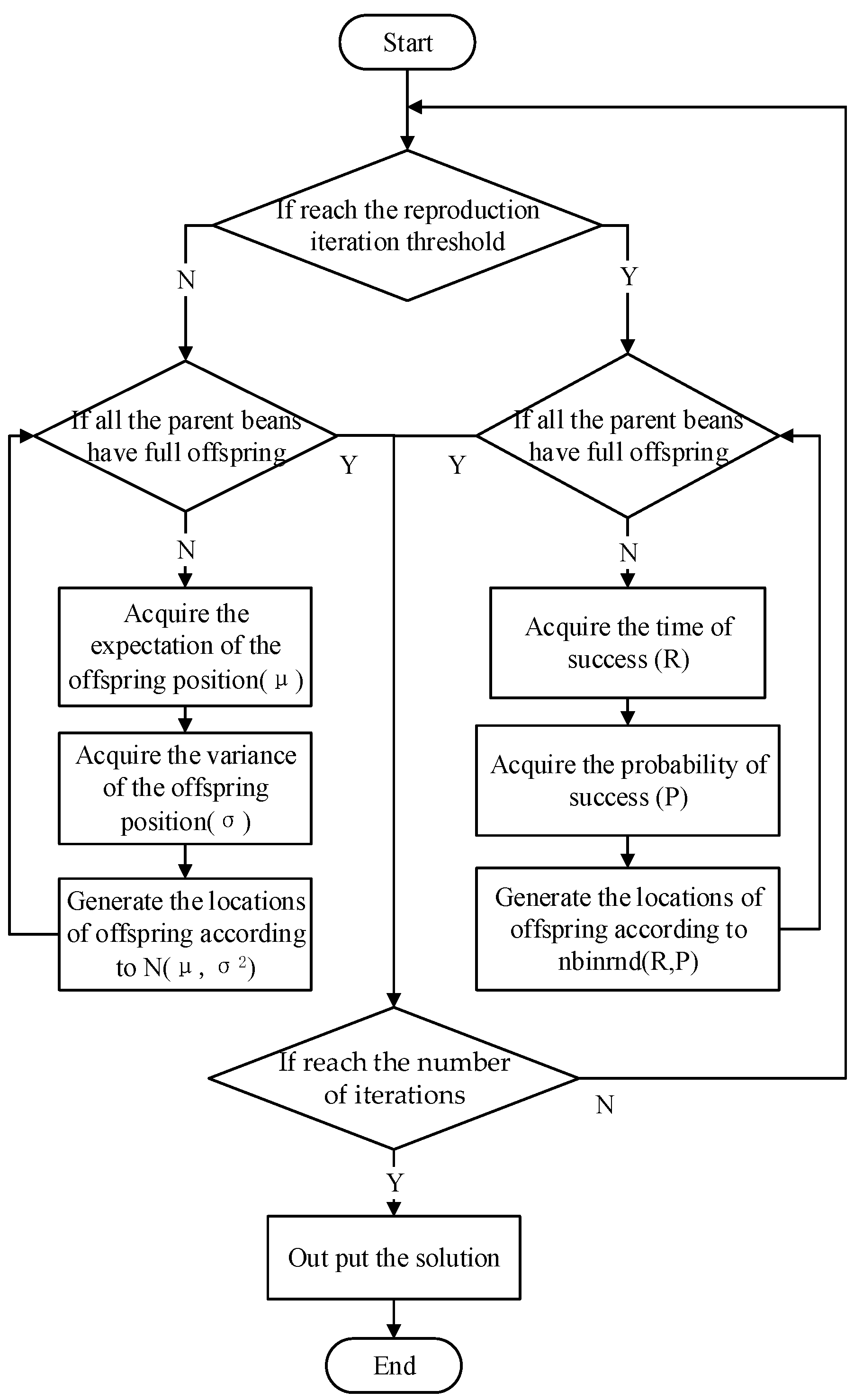
The flowchart for offspring generation by parent beans is shown as Figure 1 as follows:

In our experiments, the negative binomial distribution function nbinrnd (R, P) in MATLAB is used, in which parameter R is the number of successes, and P is the probability of success in a single trial. Both R and P may be vectors, matrixes, or multidimensional arrays with the same dimension. Some preliminary experimental results have been published in the ICSI conference proceedings [39].

To generate offspring individual beans according to a negative binominal distribution, the following process should be followed:

R = abs(F^thPop(1,:) × (100/F^thPop(1)))

(2)

Parameter P can be set as a random real number in [0, 1], theoretically, but it is better to set P according to the problems to be solved. In the experiments contained in this paper, P is set at 0.5, because the number of successes is set to the value of the current parent bean’s position. The code of the population distribution model is described as follows:

for NumPop = 1:sizepop

 if (NumPop ~= F^thIndex(1) && NumPop ~= F^thIndex(2) && NumPop ~= F^thIndex(3))

 if NumPop <= sizepop*7/10

   pop(NumPop,:) = nbinrnd(abs(F^thPop(1,:)*(100/F^thPop(1))),pnbrnd)/(100/(F^thPop(1)));

 elseif NumPop > sizepop*7/10 && NumPop <=sizepop*9/10

   pop(NumPop,:) = nbinrnd(abs(F^thPop(2,:)*(100/F^thPop(2))),pnbrnd-0.1)/(100/(F^thPop(2)));

 else

   pop(NumPop,:) = nbinrnd(abs(F^thPop(3,:)*(100/F^thPop(3))),pnbrnd)/(100/(F^thPop(3)));

 end;

 end;

end;

NumPop is a integer between 1 and sizepop; sizepop is the size of population; F^thIndex(n) is the label of the nth father bean; and pop(NumPop,:) is the position vector of the individual whose label is NumPop.

4. Experiments and Analysis

4.1. Test Functions

In the experiments, ten benchmark mathematical functions (described in

Table 2. Test functions.

Function Name	No.	Mathematical Representation (f(X))	Initial Range	Best Objective Function Value
Sphere	F1	$F_1(x)={\displaystyle \sum _{i=1}^n{x_i}^2}$	[−100, 100]n	0
Schwefel 2.22	F2	$F_2(x)={\displaystyle \sum _{i=1}^n\left|x_i\right|}+{\displaystyle \prod _{i=1}^n\left|x_i\right|}$	[−10, 10]n	0
Schwefel 1.2	F3	$F_3(x)={\displaystyle \sum _{i=1}^n{({\displaystyle \sum _{j=1}^i{x}_j})}^2}$	[−100, 100]n	0
Schwefel 2.21	F4	$F_4(x)={\max }_i\left\{\left|x_i\right|,1\le i\le n\right\}$	[−100, 100]n	0
Rosenbrock	F5	$F_5(x)={\displaystyle \sum _{i=1}^{n-1}{(100{(x_{i+1}-{x_i}^2)}^2+(x_i-1))}^2}$	[−30, 30]n	0
Quartic	F6	$F_6(x)={\displaystyle \sum _{i=1}^{n}i{x_i}^4+random[0,1)}$	[−1.28, 1.28]n	0
Schwefel 2.26	F7	$F_7(x)=-{\displaystyle \sum _{i=1}^n(x_i\sin (\sqrt{\left|x_i\right|}))}$	[−500, 500]n	−12,569.483
Rastrigin	F8	$F_8(x)={\displaystyle \sum _{i=1}^n({x_i}^2-10\cos (2\pi x_i)}+10{)}^2$	[−5.12, 5.12]n	0
Ackley	F9	$F_9(x)=-20\exp (-0.2\sqrt{\frac{1}{n}{\displaystyle \sum _{i=1}^n{x_i}^2}})-\exp (\frac{1}{n}{\displaystyle \sum _{i=1}^n\cos 2\pi x_i})+20+e$	[−32, 32]n	0
Griewank	F10	$F_{10}(x)=\frac{1}{4000}{\displaystyle \sum _{i=1}^n{(x_i)}^2}-{\displaystyle \prod _{i=1}^n\cos (\frac{x_i}{\sqrt{i}})}+1$	[−600, 600]n	0

) are used to test the effectiveness of a BOA algorithm based on a mixed-distribution model (NBOA). The dimension of every benchmark mathematical function is set to be 30 (i.e., n = 30).

4.2. Experimental Parameter Settings

Experimental parameter settings is shown in

Table 3. Experimental parameter settings.

Experimental Algorithms	Population Size	Generations
NBOA-3	50	500
NBOA-6
BOA-6
PSO

. In Table 3, NBOA-3 is an NBOA with three parent beans; NBOA-6 has six parent beans, and BOA-6 is a BOA based on a normal distribution models with six parent beans.

The parameter settings of NBOA-6 and BOA-6 are shown in

Table 4. Parameter settings of BOA-6/NBOA6.

Experimental Functions	Distance Threshold
F1	Di1 $\in$ (0, 12]; Dj2 $\in$ (0, 15]; Dk3 $\in$ (0, 15]; Dm4 $\in$ (0, 15]; D56 $\in$ (0, 15];
F2	Di1 $\in$ (0, 5]; Dj2 $\in$ (0, 5]; Dk3 $\in$ (0, 6]; Dm4 $\in$ (0,6]; D56 $\in$ (0, 6];
F3	Di1 $\in$ (0, 10]; Dj2 $\in$ (0, 10]; Dk3 $\in$ (0, 12]; Dm4 $\in$ (0, 12]; D56 $\in$ (0, 12];
F4	Di1 $\in$ (0, 10]; Dj2 $\in$ (0, 10]; Dk3 $\in$ (0, 12]; Dm4 $\in$ (0, 12]; D56 $\in$ (0, 12];
F5	Di1 $\in$ (0, 6]; Dj2 $\in$ (0, 6]; Dk3 $\in$ (0, 9]; Dm4 $\in$ (0, 9]; D56 $\in$ (0, 9];
F6	Di1 $\in$ (0, 4]; Dj2 $\in$ (0, 4]; Dk3 $\in$ (0, 5]; Dm4 $\in$ (0, 5]; D56 $\in$ (0, 5];
F7	Di1 $\in$ (0, 30]; Dj2 $\in$ (0, 30]; Dk3 $\in$ (0, 35]; Dm4 $\in$ (0, 35]; D56 $\in$ (0, 35];
F8	Di1 $\in$ (0, 3]; Dj2 $\in$ (0, 3]; Dk3 $\in$ (0, 5]; Dm4 $\in$ (0, 5]; D56 $\in$ (0, 5];
F9	Di1 $\in$ (0, 12]; Dj2 $\in$ (0, 12]; Dk3 $\in$ (0, 15]; Dm4 $\in$ (0, 15]; D56 $\in$ (0, 15];
F10	Di1 $\in$ (0, 60]; Dj2 $\in$ (0, 60]; Dk3 $\in$ (0, 80]; Dm4 $\in$ (0, 80]; D56 $\in$ (0, 80];

, in which i ∈ {2,3,4,5,6}, j ∈ {3,4,5,6}, k ∈ {4,5,6}, m ∈ {5,6}, and p_n is the threshold of population multiplication. The parameter settings of the PSO algorithm are shown in

Table 5. Parameter settings of PSO.

Experimental Functions	[Vmax,Vmin]
F1	[−1, 1]
F2	[−1, 1]
F3	[−1, 1]
F4	[−1, 1]
F5	[−0.5, 0.5]
F6	[−1, 1]
F7	[−30, 30]
F8	[−0.5, 0.5]
F9	[−1, 1]
F10	[−15, 15]

. The parameter settings of the NBOA-3 algorithm are shown in

Table 6. Parameter settings of NBOA3.

Experimental Functions	Distance Threshold
F1	D21 $\in$ (0, 12]; D31 $\in$ (0, 15]; D32 $\in$ (0, 15];
F2	D21 $\in$ (0, 5]; D31 $\in$ (0, 6]; D32 $\in$ (0, 6];
F3	D21 $\in$ (0, 10]; D31 $\in$ (0, 10]; D32 $\in$ (0, 12];
F4	D21 $\in$ (0, 10]; D31 $\in$ (0, 10]; D32 $\in$ (0, 12];
F5	D21 $\in$ (0, 6]; D31 $\in$ (0, 9]; D32 $\in$ (0, 9];
F6	D21 $\in$ (0, 4]; D31 $\in$ (0, 5]; D32 $\in$ (0, 5];
F7	D21 $\in$ (0, 30]; D31 $\in$ (0, 35]; D32 $\in$ (0, 35];
F8	D21 $\in$ (0, 3]; D31 $\in$ (0, 5]; D32 $\in$ (0, 5];
F9	D21 $\in$ (0, 12]; D31 $\in$ (0, 15]; D32 $\in$ (0, 15];
F10	D21 $\in$ (0, 60]; D31 $\in$ (0, 80]; D32 $\in$ (0, 80];

.

In Table 4, in which the value of generations in NBOA-6 is less than p_n, these settings are valid to BOA-6. The position values of 30% of the offspring beans generated are in line with the distribution normrnd (F^thPop(1,:), 1). The position values of 20% of the offspring beans generated are in line with the distribution normrnd (F^thPop(2,:), 2). The position values of 20% of the offspring beans generated are in line with the distribution normrnd (F^thPop(3,:), 2). The position values of 10% of the offspring beans generated are in line with the distribution normrnd (F^thPop(4,:), 3). The position values of 10% of the offspring beans generated are in line with the distribution normrnd (F^thPop(5,:), 3). The position values of 10% of the offspring beans generated are in line with the distribution normrnd (F^thPop(6,:), 3). When the number of generations in NBOA-6 is no less than p_n, the offspring population will be generated according to the negative binomial distribution.

Except parameter settings in Table 5; other parameters of PSO are set as follows:

w = 1/(2 × log(2));

c1 = c2 = 2.05;

In Table 6, the position values of 70% of the offspring beans generated are in line with the distribution normrnd (F^thPop(1,:), 1). The position values of 20% of the offspring beans generated are in line with the distribution normrnd (F^thPop(2,:), 1.2). The position values of 10% of the offspring beans generated are in line with the distribution normrnd (F^thPop(3,:), 1.5).

4.3. Experimental Results

Each function optimization experiment is repeated 50 times. Each algorithm runs 500 generations in each experiment. For unimodal functions F1–F6,

Table 7. Experimental results of unimodal function optimization.

Experimental Functions	Algorithms	Optimal Solutions	Average Results	SD
F1	BOA-6	1.29 × 10−14	1.21 × 10−4	4.09 × 10−4
	NBOA-3	3.42 × 10−67	1.04 × 10−14	7.37 × 10−14
	NBOA-6	1.31 × 10−33	3.84 × 10−8	2.18× 10−7
	PSO	6.97 × 10−3	3.09 × 10−2	1.88 × 10−2
F2	BOA-6	2.42 × 10−12	3.45 × 10−4	2.01 × 10−3
	NBOA-3	5.21 × 10−68	8.44 × 10−17	5.97 × 10−16
	NBOA-6	8.28 × 10−21	1.81 × 10−7	9.12 × 10−7
	PSO	5.99 × 10−1	1.99	1.04
F3	BOA-6	2.39 × 10−12	2.10 × 10−3	4.01 × 10−3
	NBOA-3	3.89 × 10−48	3.49 × 10−5	2.47 × 10−4
	NBOA-6	1.13 × 10−17	1.24 × 10−4	6.2 × 10−4
	PSO	9.34 × 10−1	3.67	1.74
F4	BOA-6	4.28 × 10−9	2.16 × 10−3	3.55 × 10−3
	NBOA-3	2.25 × 10−36	1.88 × 10−17	1.33 × 10−16
	NBOA-6	1.64 × 10−12	1.71 × 10−7	4.25 × 10−7
	PSO	3.39 × 10−1	8.77 × 10−1	4.81 × 10−1
F5	BOA-6	2.88 × 10	2.89 × 10	8.89 × 10−2
	NBOA-3	2.86 × 10	2.89 × 10	1.31 × 10−1
	NBOA-6	2.86 × 10	2.92 × 10	6.79 × 10−1
	PSO	2.28 × 10	3.92 × 10	2.93 × 10
F6	BOA-6	4.79 × 10−5	9.89 × 10−4	6.63 × 10−4
	NBOA-3	1.19 × 10−5	7.15 × 10−4	6.22 × 10−4
	NBOA-6	5.62 × 10−5	6.90 × 10−4	6.28 × 10−4
	PSO	2.64 × 10−2	6.82 × 10−2	3.38 × 10−2

lists the optimal results, average results, and the corresponding standard deviations for all the algorithms. For multimodal functions F7–F10,

Table 8. Experimental results of multimodal function optimization.

Experimental Functions	Algorithms	Optimal Solutions	Average Results	SD
F7	BOA-6	−9.091 × 103	−7.94 × 103	6.41 × 102
	NBOA-3	−8.99 × 103	−7.28 × 103	7.04 × 102
	NBOA-6	−1.11 × 104	−7.80 × 103	7.55 × 102
	PSO	−7.69 × 103	−6.09 × 103	6.39 × 102
F8	BOA-6	1.61 × 10−8	1.62 × 10−3	3.07 × 10−3
	NBOA-3	2.11 × 10−7	8.04 × 10−4	1.97 × 10−3
	NBOA-6	1.36 × 10−9	5.27 × 10−4	1.41 × 10−3
	PSO	9.63	2.79 × 10	8.74
F9	BOA-6	7.71 × 10−6	2.58 × 10−3	4.37 × 10−3
	NBOA-3	1.15 × 10−13	5.32 × 10−6	3.76 × 10−5
	NBOA-6	2.58 × 10−14	5.60 × 10−9	2.21 × 10−8
	PSO	2.02	3.89	8.18 × 10−1
F10	BOA-6	7.01 × 10−8	3.90 × 10−4	8.64 × 10−4
	NBOA-3	1.52 × 10−8	1.94 × 10−4	4.57 × 10−4
	NBOA-6	1.59 × 10−9	1.18 × 10−4	2.83 × 10−4
	PSO	4.31 × 10−5	1.65 × 10−4	8.35 × 10−5

lists the optimal results, average results, and the corresponding standard deviations for all the algorithms.

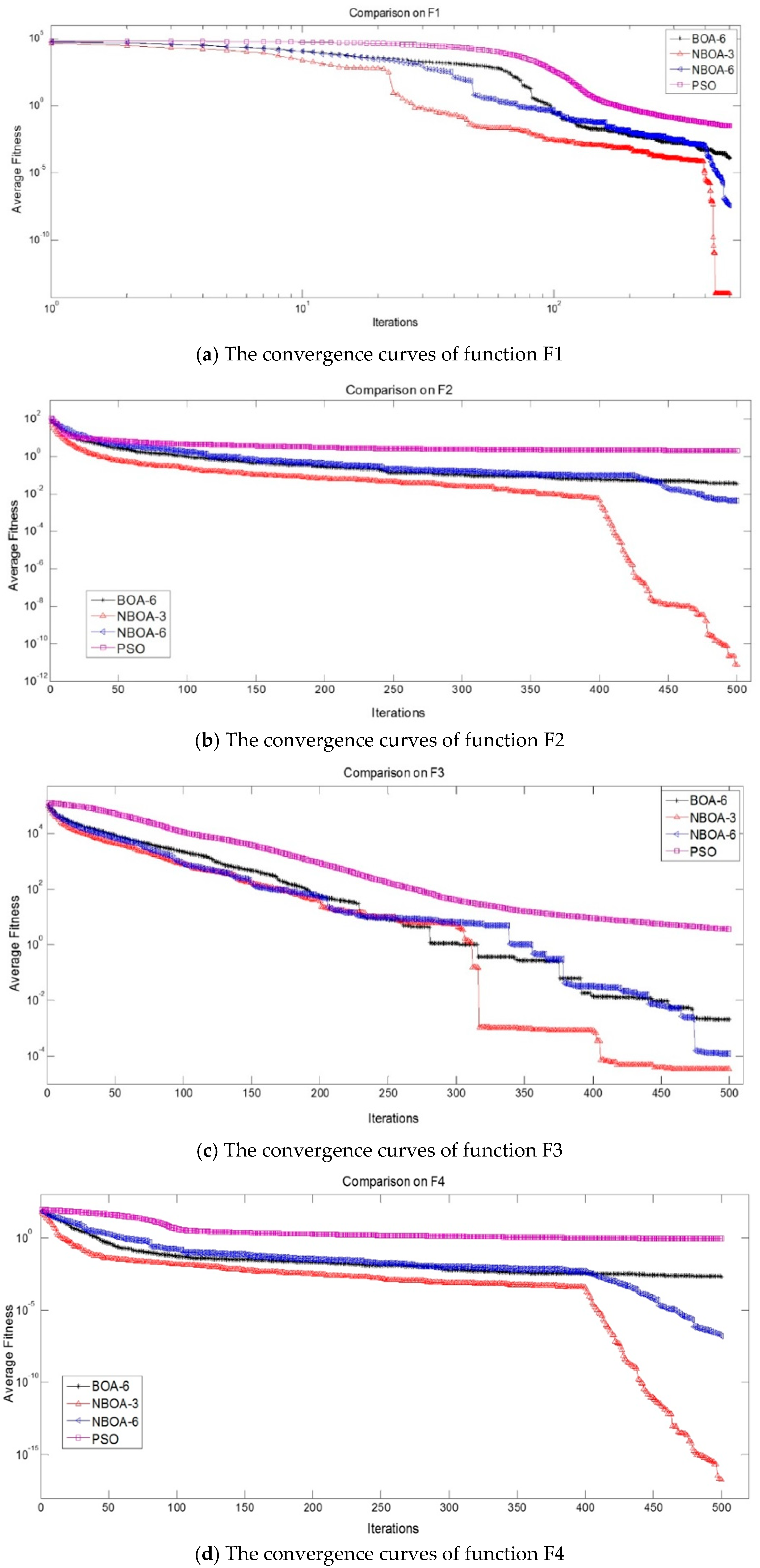
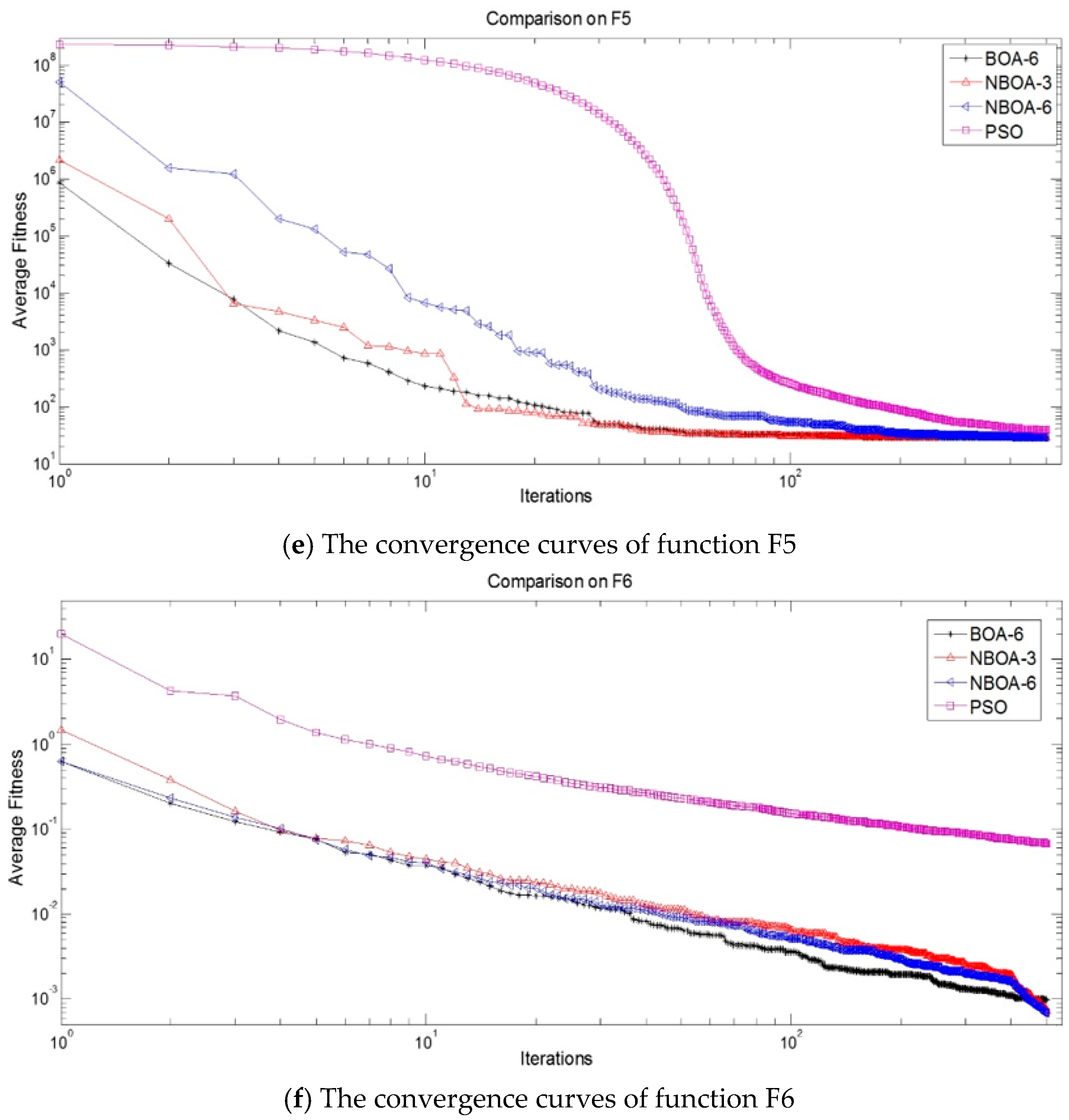
The convergence curves (NBOA-3, NBOA-6, BOA-6, and PSO) of unimodal function optimisation are as follows:

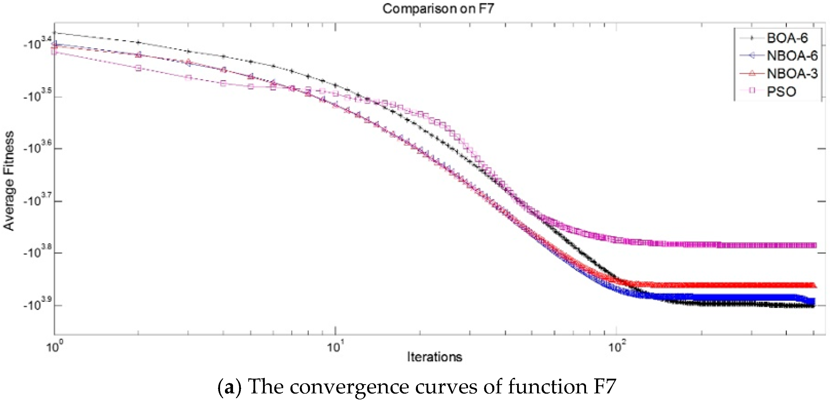
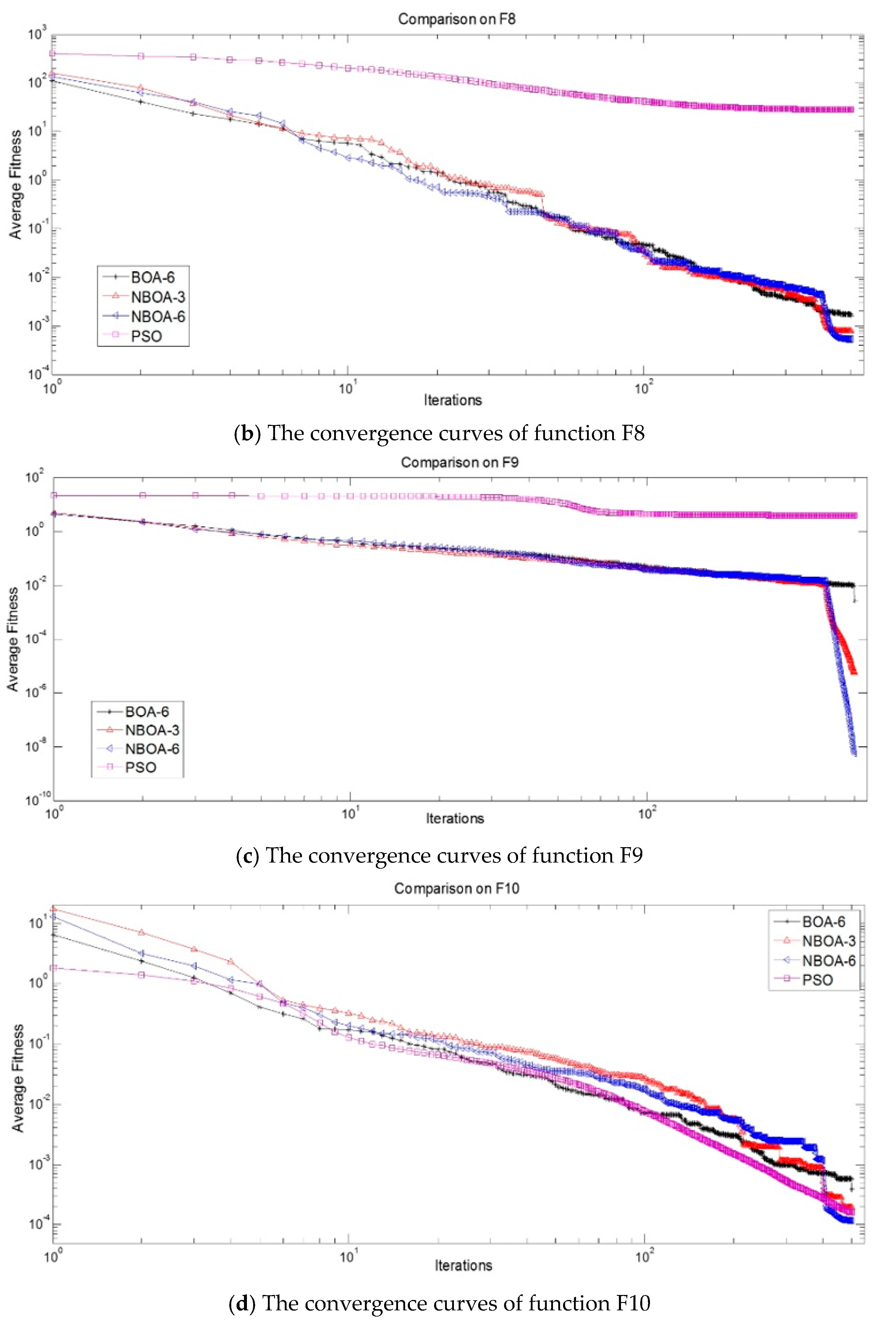
The convergence curves (NBOA-3, NBOA-6, BOA-6, and PSO) of multimodal function optimisation are shown as follows.

4.4. Experiment Analysis

We will analyse the experimental results in terms of optimal and average results, as follows.

4.4.1. Statistical Results

• Optimal Results

The optimal result is the best result of an algorithm that runs 50 times. In Table 7, SD represents the standard deviation, which measures the amount of variation around the mean. We can see from the above results in Table 7 and Table 8 that NBOA-3 obtains relative optimal results for six functions (F1, F2, F3, F4, F5, and F6). NBOA6 obtains relative optimal results for four functions (F7, F8, F9, and F10). The performance of BOA-6 is, relatively speaking, not very good but compared with the algorithms PSO and BOA-3, there is evidence of improvement.

• Average Results

Average results are the average of 50 algorithm runs. In the experiments, NBOA-3 obtained the best average results for five functions: F1, F2, F3, F4, and F5. NBOA-6 obtained the best average results for four functions: F6, F8, F9, and F10. BOA-6 obtained the best average results for functions F5 and F7.

4.4.2. Analysis of Results

• 1. Unimodal Functions Optimisation Analysis

We can see from the above statistics and convergence curves (Figure 2) that NBOA-3 obtained the best solution in most of the unimodal function optimisations. Our conclusions are that:

(1)

Because the population sizes of the four algorithms are same, the highest number of offspring dominated by parent beans occurred in algorithm NBOA-3. For example, the No. 1 parent bean in algorithm NBOA-3 dominated 70% of individual offspring and distributed them according to its wish. However, the No. 1 parent bean in algorithm NBOA-6 only dominated 30% of the offspring. Therefore, algorithm NBOA-3 can approximate the optimal solution (or the local optimal solution) more quickly in theory. This is largely consistent with the experimental results. Hence, better results appear to be given by algorithm NBOA-3.

(2)

Considering unimodal function optimisation, the mutation mechanism of individuals follows the method:

pop(rndi,:) = (rands(1,nn)) × pop(ceil(rand × nn)),

(3)

The random sowing method strongly increases the global optimisation ability in later periods of evolution. It makes the excellent algorithm even better.

(3)

The model based on the binomial distribution can effectively increase the optimisation ability of the algorithm. A decreasingly steep slope is evident in the comparative figures of algorithm convergence performance (Figure 2). It is the location of the steep slope that starts using the binomial distribution model in BOA. It is evident that the model based on the binomial distribution enhances the performance of NBOA-3 and NBOA-6.

• 2. Multimodal Functions Optimisation Analysis

In most of the multimodal-function optimisations, NBOA-6 obtained the best solutions. From the algorithm experiment results and the and convergence curves (Figure 3) shown above, we can analyse the results as follows:

(1)

Because the distances (Euclidean distances are used in the experiments) between the parent beans need to meet the threshold set before the experiments, the more parent beans there are, the more advantageously parent beans can explore the problem domain space. That is to say, there are more opportunities to quickly find better problem areas that effectively enhance the algorithm’s ability to achieve global optimisation.

(2)

For multimodal function optimisation, the mechanism of individual bean variation adopts the following method:

pop(NumPop,:) = (rands(1,nn)) × (popmax − (popmax − popmin) × rand)

(4)

This method simulates the phenomenon of accidental seed migration in nature and further enhances the ability to achieve global optimisation.

(3)

As mentioned above, because the model based on the negative binomial distribution is used in algorithm NBOA-6, its optimisation ability is better than that of algorithm BOA-6.

5. Conclusions

Inspired by the spatial distribution pattern and the adaptive phenomena of plants in nature, a novel evolutionary algorithm named BOA was proposed. This paper first introduced the negative binomial distribution. By processing the distribution’s variables, the distribution can be converted into a model of a population distribution for solving continuous optimisation problems. In combination with the normal distribution, a novel kind of BOA based on a mixed distribution model was proposed. Ten benchmark mathematical function optimisation experiments were carried out to test its effectiveness. By comparing and analysing the experimental results obtained from the experiments of four algorithms (BOA-6, NBOA-3, NBOA-6, and PSO), we can reach a conclusion that the negative binomial distribution model is effective.

In BOA research, three kinds of population distribution models have been proposed for improving the effectiveness of BOA algorithms. However, in the area of biostatistical research, this is only a very small number of the many possible biological spatial distribution patterns that occur in nature. There are still many distribution models that can be used to construct population distribution models for BOA, such as the Neyman distribution and Polya-Eggenberger distribution. In addition, there is currently research into combining these algorithms with other intelligent algorithms. However, it is not carried out in BOA, such as the crossover operator of Genetic Algorithm and information feedback models. In the future, we will continue the research of BOA and its applications. We also hope that other researchers will give more attention to BOA and carry out related research work.

References

- Yang, B. Cooperative Control for Swarm Robots based on Bio-Inspired Intelligent Algorithms. Ph.D. Thesis, Donghua University, Shanghai, China, 2016. [Google Scholar]
- Bonyadi, M.R.; Michalewicz, Z. Particle Swarm Optimization for Single Objective Continuous Space Problems: A Review. Evolut. Comput. 2017, 25, 1–54. [Google Scholar] [CrossRef] [PubMed]
- Chen, Z.; Zhou, S.; Luo, J. A robust ant colony optimization for continuous functions. Expert Syst. Appl. 2017, 81, 309–320. [Google Scholar] [CrossRef]
- Zhu, X.; Ni, Z.; Cheng, M.; Li, J.; Jin, F.; Ni, L. Haze prediction method based on multi-fractal dimension and co-evolution discrete artificial fish swarm algorithm. Syst. Eng. Theory Pract. 2017, 37, 999–1010. [Google Scholar]
- Kalin, P. Free Search—Comparative analysis 100. Int. J. Metaheuristics 2014, 3, 118–132. [Google Scholar]
- Montiela, O.; Castillob, O.; Melinb, P.; Rodríguez Díazc, A.; Sepúlvedaa, R. Human evolutionary model: A new approach to optimization. Inf. Sci. 2007, 177, 2075–2098. [Google Scholar] [CrossRef]
- He, S.; Wu, Q.H.; Saunders, J.R. Group search optimizer: An optimization algorithm inspired by animal searching behavior. IEEE Trans. Evolut. Comput. 2009, 13, 973–990. [Google Scholar] [CrossRef]
- Hussein, W.A.; Sahran, S.; Abdullah, S.N.H.S. The variants of the Bees Algorithm (BA): A survey. Artif. Intell. Rev. 2017, 47, 67–121. [Google Scholar] [CrossRef]
- Yang, C.; Ji, J.; Liu, J.; Yin, B. Bacterial foraging optimization using novel chemotaxis and conjugation strategies. Inf. Sci. 2016, 363, 72–95. [Google Scholar] [CrossRef]
- Eusuff, M.; Lansey, K.; Pasha, F. Shuffled frog-leaping algorithm: A memetic meta-heuristic for discrete optimization. Eng. Optim. 2006, 38, 129–154. [Google Scholar] [CrossRef]
- Tan, Y.; Yu, C.; Zheng, S.; Ding, K. Introduction to Fireworks Algorithm. Int. J. Swarm Intell. Res. 2013, 4, 39–70. [Google Scholar] [CrossRef]
- Wang, G.G.; Tan, Y. Improving Metaheuristic Algorithms with Information Feedback Models. IEEE Trans. Cybern. 2017, 99, 1–14. [Google Scholar] [CrossRef]
- Wang, G.G.; Cai, X.; Cui, Z.; Min, G.; Chen, J. High Performance Computing for Cyber Physical Social Systems by Using Evolutionary Multi-Objective Optimization Algorithm. IEEE Trans. Emerg. Top. Comput. 2017. [Google Scholar] [CrossRef]
- Wang, G.G.; Guo, L.; Gandomi, A.H.; Hao, G.-S.; Wang, H. Chaotic Krill Herd algorithm. Inf. Sci. 2014, 274, 17–34. [Google Scholar] [CrossRef]
- Wang, G.G.; Gandomi, A.H.; Alavi, A.H.; Gong, D. A comprehensive review of krill herd algorithm: Variants, hybrids and applications. Artif. Intell. Rev. 2017. [Google Scholar] [CrossRef]
- Wang, G.G.; Gandomi, A.H.; Chu, H.C.; Zhao, X. Hybridizing harmony search algorithm with cuckoo search for global numerical optimization. Soft Comput. 2016, 20, 273–285. [Google Scholar] [CrossRef]
- Wang, G.G.; Deb, S.; Cui, Z. Monarch Butterfly Optimization. Neural Comput. Appl. 2015. [Google Scholar] [CrossRef]
- Wang, G.G. Moth search algorithm: A bio-inspired metaheuristic algorithm for global optimization problems. Memet. Comput. 2016. [Google Scholar] [CrossRef]
- Wang, G.G.; Deb, S.; Gandomi, A.H.; Zhang, Z.; Alavi, A.H. Chaotic cuckoo search. Soft Comput. 2016, 20, 3349–3362. [Google Scholar] [CrossRef]
- Eiben, A.E. In vivo veritas: Towards the evolution of things. Lect. Notes Comput. Sci. 2014, 8672, 24–39. [Google Scholar]
- Geng, J.C.; Cui, Z.; Gu, X.S. Scatter search based particle swarm optimization algorithm for earliness/tardiness flowshop scheduling with uncertainty. Int. J. Autom. Comput. 2016, 13, 285–295. [Google Scholar] [CrossRef]
- Lazzús, J.A.; Rivera, M.; López-Caraballo, C.H. Parameter estimation of Lorenz chaotic system using a hybrid swarm intelligence algorithm. Phys. Lett. A 2016, 380, 1164–1171. [Google Scholar] [CrossRef]
- Dadgar, M.; Jafari, S.; Hamzeh, A.A. PSO-based multi-robot cooperation method for target searching in unknown environments. Neurocomputing 2016, 177, 62–74. [Google Scholar] [CrossRef]
- Ghaemi, M.; Feizi-Derakhshi, M.R. Feature selection using Forest Optimization Algorithm. Pattern Recognit. 2016, 60, 121–129. [Google Scholar] [CrossRef]
- Garcia, M.A.P.; Montiel, O.; Castillo, O.; Melin, P. Path planning for autonomous mobile robot navigation with ant colony optimization and fuzzy cost function evaluation. Appl. Soft Comput. 2009, 9, 1102–1110. [Google Scholar] [CrossRef]
- Couceiro, M.S.; Figueiredo, C.M.; Rui, P.R.; Ferreira, N.M.F. Darwinian Swarm Exploration under Communication Constraints: Initial Deployment and Fault-Tolerance Assessment. Robot. Auton. Syst. 2014, 62, 528–544. [Google Scholar] [CrossRef]
- Zhang, X.; Wang, R.; Song, L. A novel evolutionary algorithm—Seed optimization algorithm. Pattern Recognit. Artif. Intell. 2008, 21, 677–681. [Google Scholar]
- Zhang, X.; Sun, B.; Mei, T.; Wang, R. A novel evolutionary algorithm inspired by beans dispersal. Int. J. Comput. Intell. Syst. 2013, 6, 79–86. [Google Scholar] [CrossRef]
- Wang, P.; Cheng, Y. Relief supplies scheduling based on bean optimization algorithm. Econ. Res. Guide 2010, 8, 252–253. [Google Scholar]
- Zhang, X.; Sun, B.; Mei, T.; Wang, R. Post-disaster restoration based on fuzzy preference relation and bean optimization algorithm. In Proceedings of the 2010 IEEE Youth Conference on Information Computing and Telecommunications (YC-ICT), Beijing, China, 28–30 November 2010; pp. 253–256. [Google Scholar]
- Zhang, X.; Wang, H.; Sun, B.; Li, W.; Wang, R. The Markov model of bean optimization algorithm and its convergence analysis. Int. J. Comput. Intell. Syst. 2013, 6, 609–615. [Google Scholar] [CrossRef]
- Li, Y. Solving TSP by an ACO-and-BOA-based Hybrid Algorithm. In Proceedings of the 2010 International Conference on Computer Application and System Modeling, Taiyuan, China, 22–24 October 2010; pp. 189–192. [Google Scholar]
- Zhang, X.; Jiang, K.; Wang, H. An improved bean optimization algorithm for solving TSP. Lect. Notes Comput. Sci. 2012, 7331, 261–267. [Google Scholar]
- Feng, T. Study and Application of Bean Optimization Algorithm on Complex Problem. Master’s Thesis, University of Science and Technology of China, Hefei, China, 2017. [Google Scholar]
- Zhang, X.; Feng, T. Chaotic bean optimization algorithm. Soft Comput. 2018, 22, 67–77. [Google Scholar] [CrossRef]
- Guoyu, L.; Ruide, L. Brief introduction of spatial methods to distribution patterns of population. J. Northwest For. Univ. 2003, 18, 17–21. [Google Scholar]
- Hao-tao, L. Introduction to studies of the pattern of plant population. Chin. Bull. Bot. 1995, 12, 19–26. [Google Scholar]
- Fei, S.-M.; He, Y.-P.; Chen, X.-M.; Jiang, J.-M.; Guo, Z.-H. Quantitative features of populations of Pinus tabulaeformis and P. armandii regenerated following water damage at Qinling Mountain China. Chin. J. Plant Ecol. 2008, 32, 95–105. [Google Scholar]
- Feng, T.; Xie, Q.; Hu, H.; Song, L.; Cui, C.; Zhang, Z. Bean optimization algorithm based on negative Binomial Distribution. Lect. Notes Comput. Sci. 2015, 9140, 82–88. [Google Scholar]
Figure 1.
Flowchart for generating offspring.
Figure 2.
The convergence curves of unimodal functions: The curves of BOA-6 are black, the curves of NBOA-6 are blue, the curves of NBOA-3 are red, and the curves of PSO are purple. All the curves are average convergence curves for 50 computational iterations, and in order to show the curves more clearly, the coordinates were changed by logarithmic processing.
Figure 3.
The convergence curves of multimodal functions: The curves of BOA-6 are black, the curves of NBOA-6 are blue, the curves of NBOA-3 are red, and the curves of PSO are purple. All the curves are average convergence curves for 50 computational iterations, and in order to show the curves more clearly, the coordinates were changed by logarithmic processing.