Development of Proportional Pressure Control Valve for Hydraulic Braking Actuator of Automobile ABS

Abstract

This research developed a novel proportional pressure control valve for an automobile hydraulic braking actuator. It also analyzed and simulated solenoid force of the control valves, and the pressure relief capability test of electromagnetic thrust with the proportional valve body. Considering the high controllability and ease of production, the driver of this proportional valve was designed with a small volume and powerful solenoid force to control braking pressure and flow. Since the proportional valve can have closed-loop control, the proportional valve can replace a conventional solenoid valve in current brake actuators. With the proportional valve controlling braking and pressure relief mode, it can narrow the space of hydraulic braking actuator, and precisely control braking force to achieve safety objectives. Finally, the proposed novel proportional pressure control valve of an automobile hydraulic braking actuator was implemented and verified experimentally.

1. Introduction

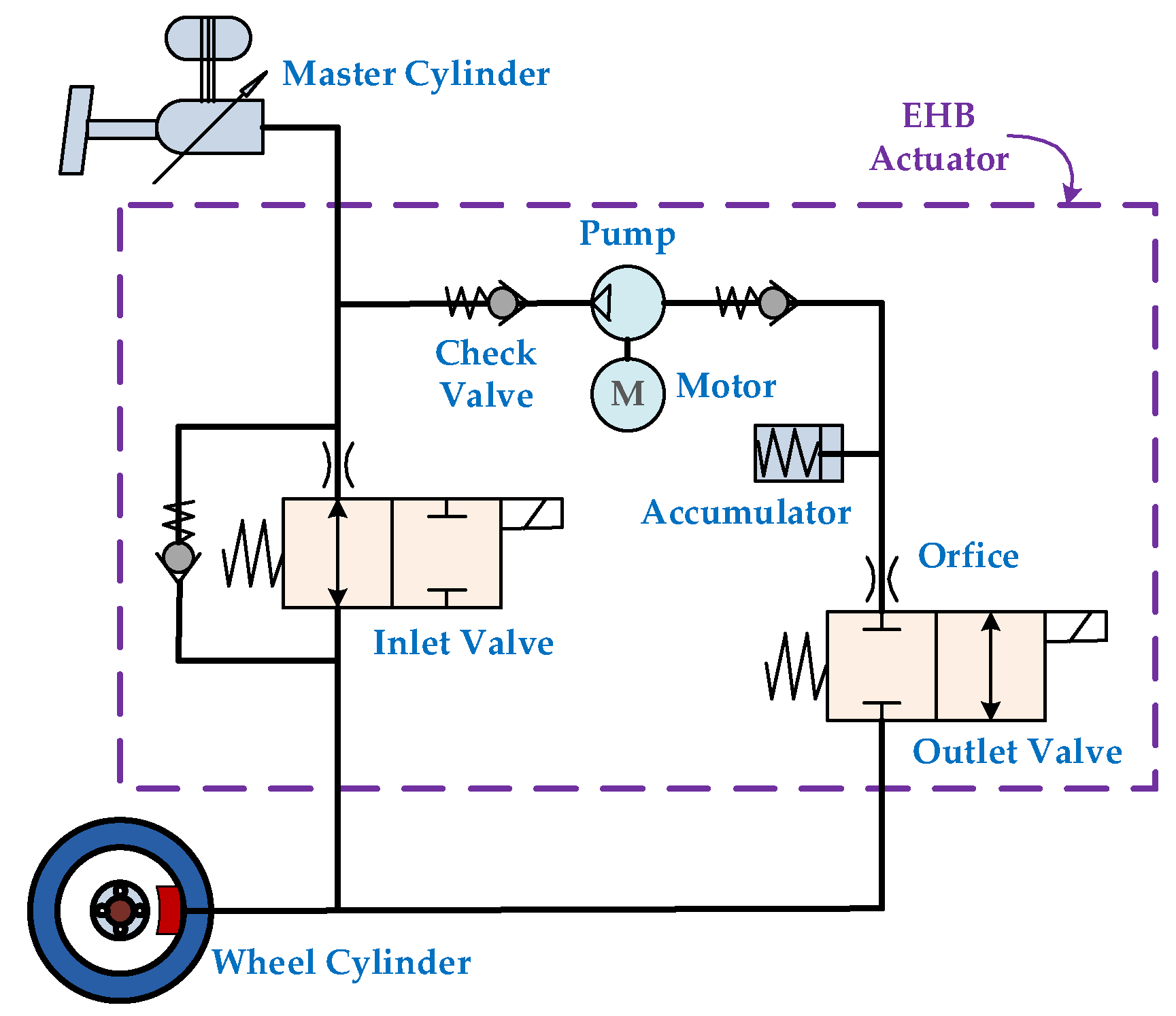
To provide safer and more comfortable driving conditions for motorists, the anti-lock braking system (ABS) is currently basic equipment for automobiles. This system achieves improved control capability by connecting the electro-hydraulic brake (EHB) between master cylinder and wheel cylinder. As ABS starts to work, the hydraulic pressure (braking force) within the tire calipers is controlled by four groups of solenoid valves (inlet/outlet valve). Furthermore, there are three patterns of pressure variation, namely pressure increase, pressure holding, and pressure decrease [1,2,3,4]. The hydraulic circuit of an EHB actuator is shown in Figure 1 [5].

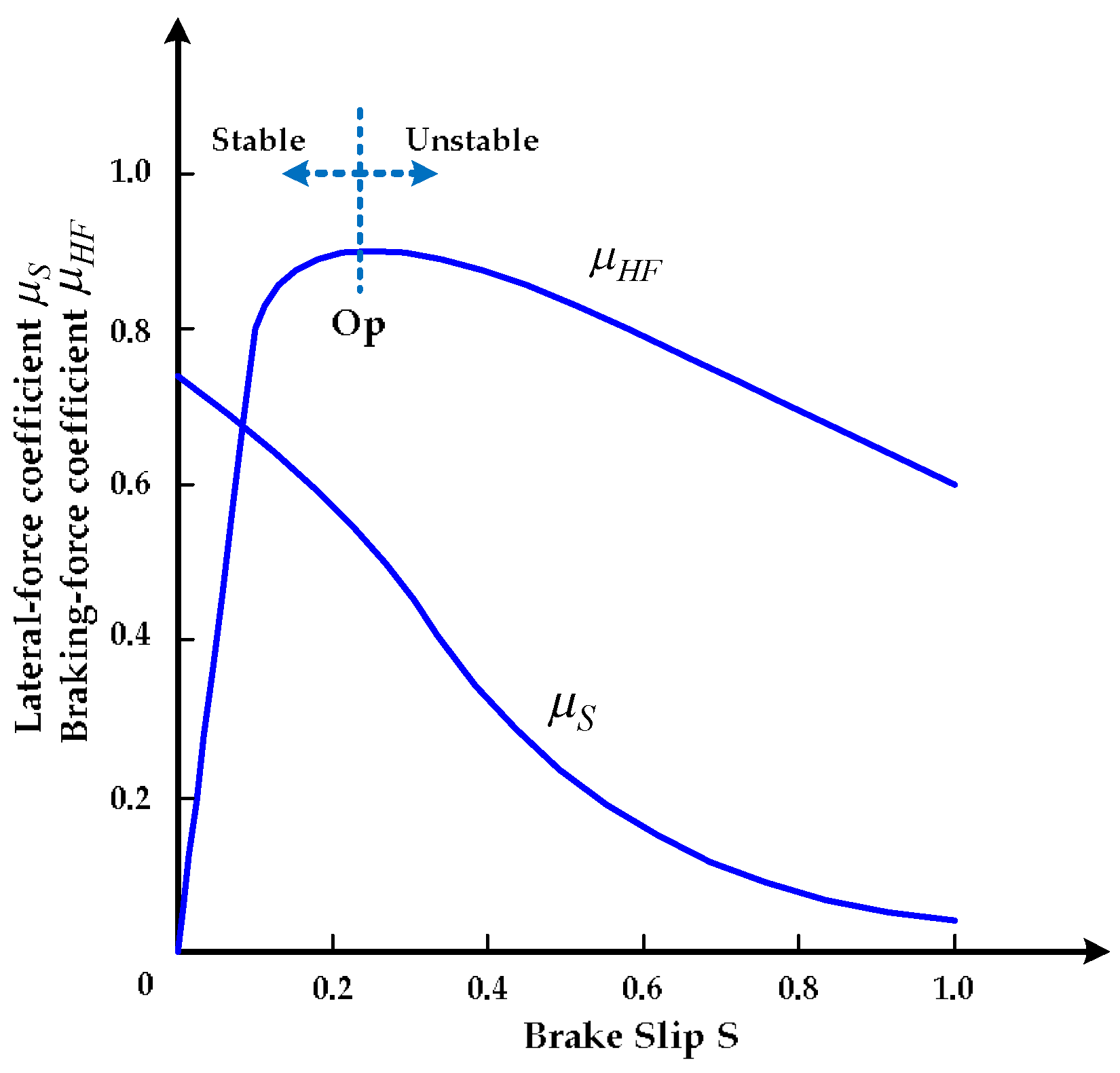
The braking capability of automobiles relies on characteristics of the tires, which are the only contact with the ground. The main factor determining this capability is the slip ratio of the tires and ground, defined as slip.

$$S=\frac{V_v-V_w}{V_v}$$

(1)

where $S$ is the slip, $V_v$ is the vehicle speed, and $V_w$ is the wheel speed.

When the slip is between 0.1 and 0.3, the braking action is most effective, and, if the slip is zero, the wheels are operating with no resistance. However, when slip is more than 0.3, the braking force may be reduced. The tires are completely locked when slip is 1, and the wheels would slide along the pavement [6,7,8,9,10,11]. The results are shown in Figure 2 [12].

An ABS braking system can prevent the improper sliding of tires and it has three functions:

(1)

When encountering an obstacle or any road conditions, it can be actuated by the steering wheel to obtain suitable tracking performance.

(2)

It can avoid excessive braking effects that can cause uncontrolled steering (if the front wheels are locked) or drifting (if the rear wheels are locked)

(3)

The electronic control braking effects can shorten the stopping distance.

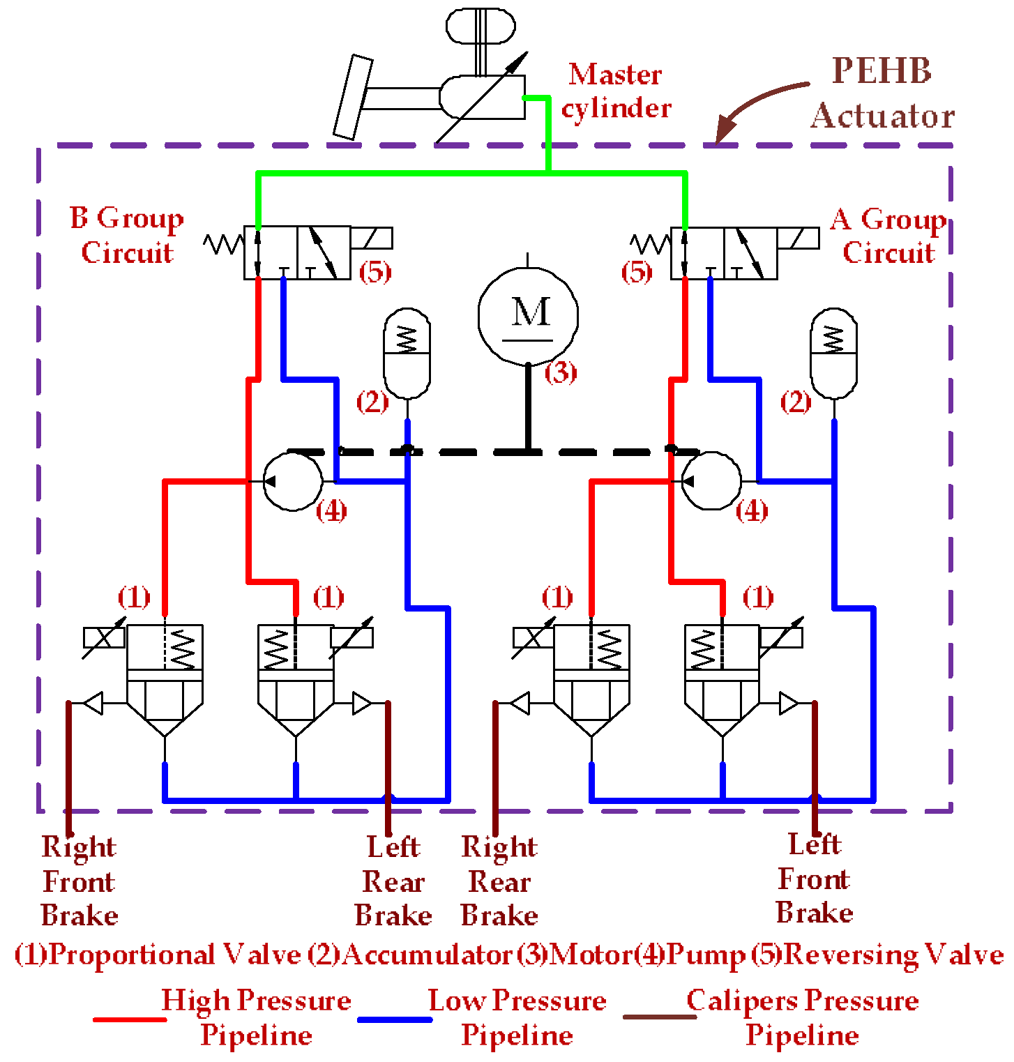
The general ABS drives the solenoid valve when it detects that the wheels are locked, and it operates the slip control in an on–off mode to release the calipers’ pressure. Traditional solenoid valve patterns can only adjust the calipers’ pressure through a fully open or closed valve port and have no accurate control for slip, so they cannot provided highly effective braking. However, an accident can occur when the ABS is actuating and high frequency vibration from the pedal make the driver panic and then release the pedal. To develop a brake actuator that uses a new pattern, and also considering the market differentiation and product performance, for the first time, a proportional pressure control valve was used for ABS to replace two solenoid valves. To improve the disadvantages of solenoid valve and achieve better slip control, the pressure to be released as determined by the corresponding input current and electromagnetic force. To improve braking quality, it can effectively control the calipers’ pressure and then decide the appropriate braking force due to the stability of pressure release control, and no pressure oscillations are generated, as with a solenoid valve. A single proportional valve for each of the four wheels was substituted for the original two solenoid valves for each wheel. This reduces the cost and space requirements compared to the traditional EHB configuration. Figure 3 shows the novel hydraulic circuit for a proportional electro-hydraulic brake (PEHB) actuator.

This research focused on the configuration design of the proportional electromagnet within the proportional valve, and its main function is to drive the armature. The development process was divided into three stages:

(1)

Firstly, using electromagnetic theory and mathematical calculations, parameters of the new cone proportional electromagnet were analyzed, and then the electromagnet force using a simulation program was estimated.

(2)

Secondly, according to the configuration design (post-analysis), the production and electromagnet force test were completed.

(3)

Thirdly, the proportional valve was tested, and its relief pressure control capability for ABS control applications of the PEHB actuator was confirmed.

2. Analysis of Proportional Solenoid Force

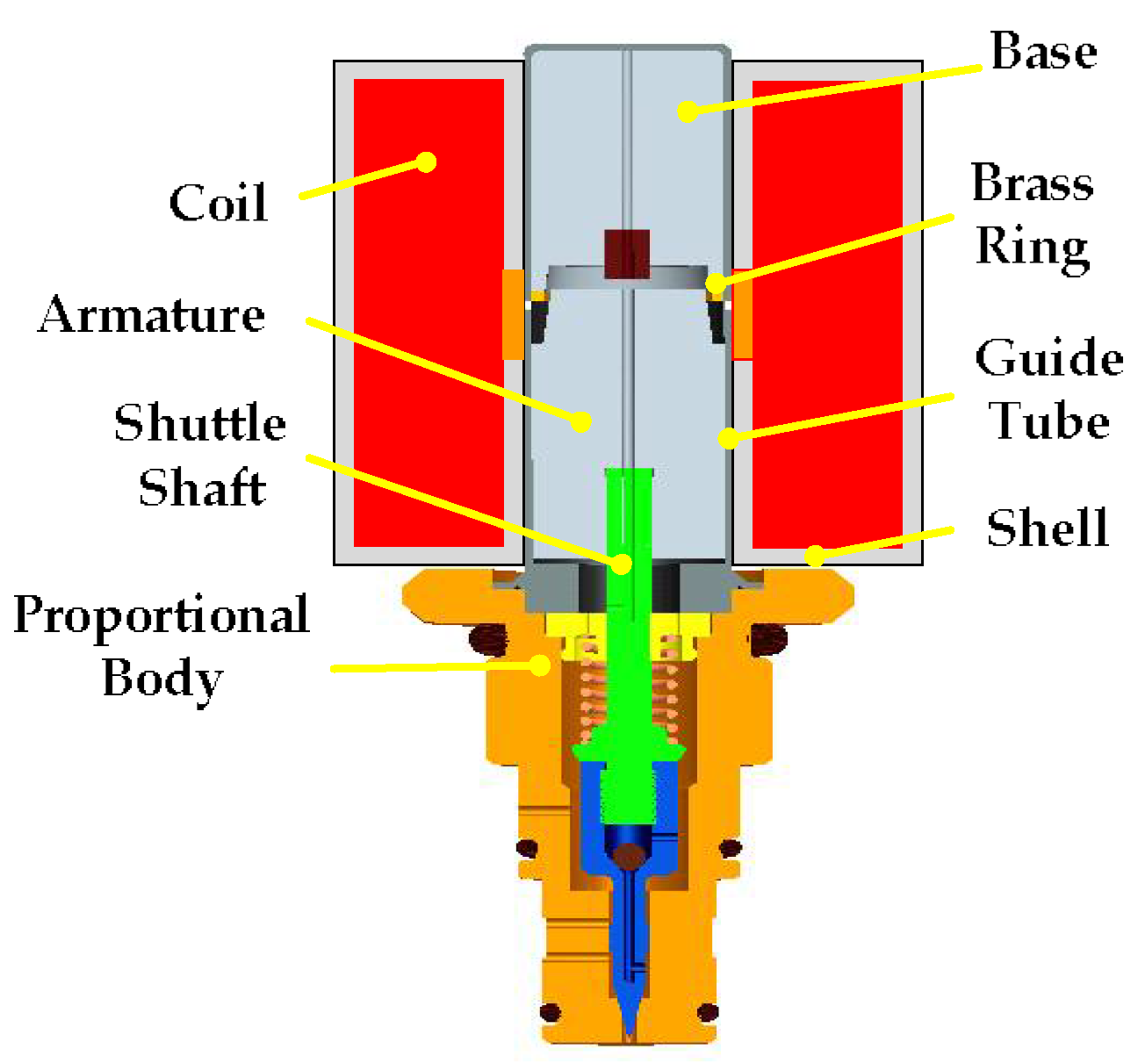
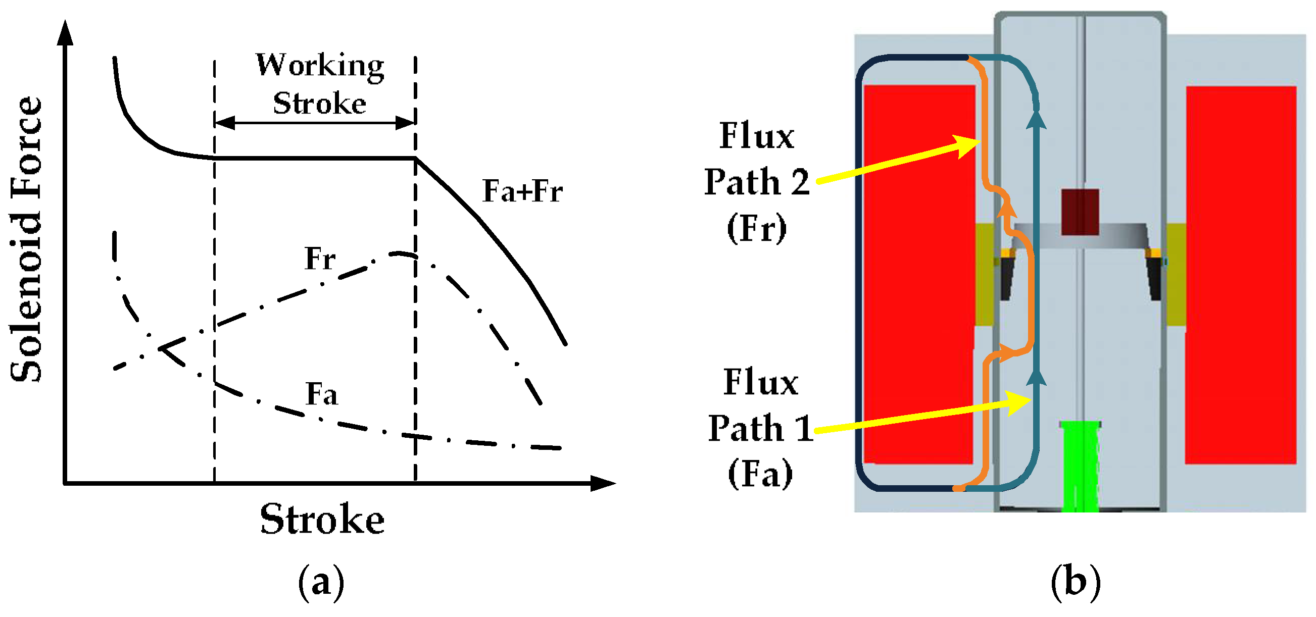
The principles of proportional valve operation are as follows. The proportional solenoid configuration (increase brass ring) can produce a horizontal solenoid force working zone which is not related to the stroke. When different currents are input, the solenoid force balances the oil pressure and the spring force. Base and armature attract each other by coil excitation, and the required stroke can be generated to drive the shuttle shaft to open the valve. Configuration of the proportional pressure valve is shown in Figure 4 [13]. This gives it two advantages: a closed-loop control (compared to the solenoid valve) and lower cost (compared to the servo valve). Figure 5 shows the axial force (Fa) of the base (flux path 1) and the radial force (Fr) of the flange (flux path 2) work with each other in specific section so that the solenoid force is equal to their sum. Therefore, the solenoid force is unrelated to the working stroke, which is why the linear proportional valve zone is formed. Therefore, the proportional electromagnet can be directly controlled, and the solenoid force depends on the operating current in the linear zone.

2.1. Permeance of Air Gaps

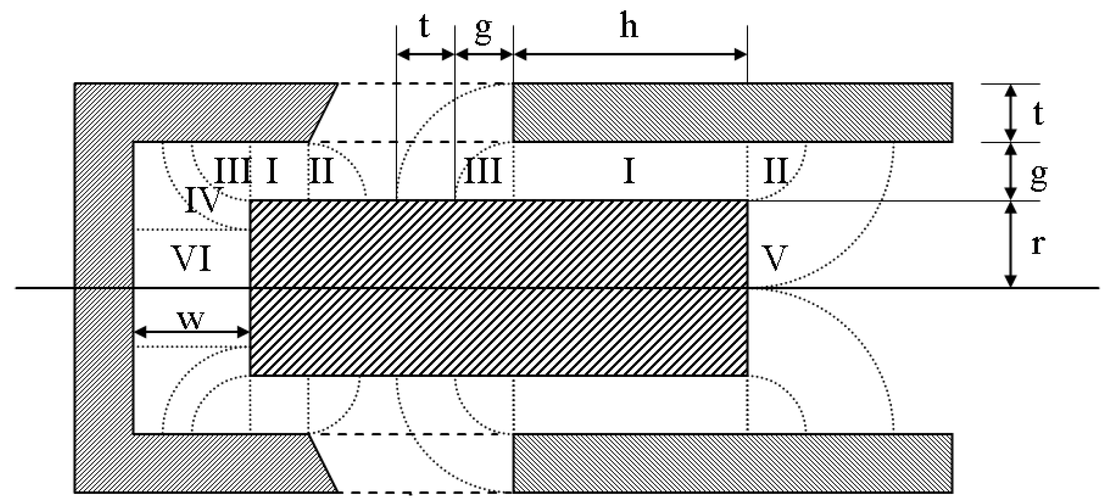
When the electromagnetic coil is energized, the energy can generate a magnetic field. Thus, there will be a group of closed magnetic circuits around the coils within the proportional solenoid, and the magnetic field intensity changes with the armature position. Lastly, it drives the armature to move according to the high magnetic energy. The basic proportional electromagnet is shown in Figure 6. Simplifying the six types of magnetic path can be the basis for subsequent calculations [14,15], as shown in

Table 1. The air gaps flux path model calculations.

Flux Path Model	Mean Path Length	Permeance ($\mathit{P}$)
I	$g$	$\frac{2\pi {\mu }_{0}h}{g}(r+\frac{g}{2})$
II	$1.22g$	$3.315{\mu }_0(r+\frac{g}{2})$
III	$1.22g$	$3.315{\mu }_0(r+\frac{g}{2})$
IV	$\sqrt{g(g+t)}$	$4{\mu }_0(r+\sqrt{g(g+t)})\ln (\frac{g+t}{g})$
V	$\sqrt{g(g+r)}$	$4{\mu }_0(r+g-\sqrt{g(g+r)})\ln (\frac{g+r}{g})$
VI	$w$	$\frac{{\mu }_0\pi }{w}{(r+g-\frac{2w}{\pi })}^2$

. Here, ${\mu }_0$ represents the permeability of air, $g$ represents the air gap, $r$ represents the armature radius, $h$ represents the right side distance between armature and brass ring, $t$ represents the thickness of brass ring, and $w$ represents the distance from base to brass ring.

2.2. Permeability of Air of the Proportional Electromagnet

For ease of construction, the metal cone replaces the traditional brass ring in this study (when the taper angle is zero, it becomes the traditional shape, and the difference between armature and base diameter is the air gap) [16]. The magnetic field lines pass in and out of the coil along the closed path and they have the same physical characteristics with current and resistance. Then, the magnetic flux moves toward the minimum reluctance. When the metals are magnetic and in contact with each other, the magnetic field lines are distributed on the surface of the metals and the air gap permeance can be ignored. When the metals are not in contact with each other, the magnetic field lines are forced to be in and out the air gaps and the directions are both vertical to the metal surface following the shortest path and minimum reluctance.

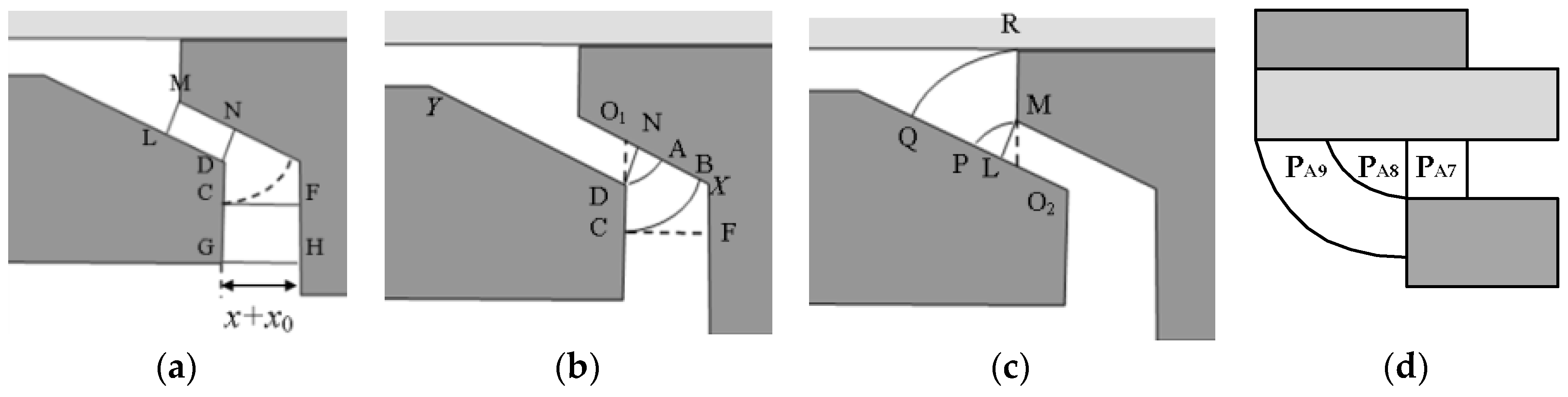
According to the proportional electromagnetic configuration of this study, the air-gap zones located at both ends of the armature are $P_{A1}$–$P_{A6}$ and $P_{A7}$–$P_{A9}$. Around the front end gap, magnetism exists between base and armature, and the direction of flow is from base to armature. An enlarged view of this is shown in Figure 7. In Figure 7a, range CFHG represents Path Mode VI, and range DLMN represents Path Mode I. In Figure 7b, range ABCD represents Path Mode IV, and range AND represents Path Mode III. In Figure 7c, range MPQR represents Path Mode V, and range LMP represents Path Mode II.

For derivation of the rear end gap, magnetism is the same as front end gap, but the direction of flow is from armature to coil base. An enlarged view is shown in Figure 7d. Permeance $P_{A7}$ represents Path Mode I, permeance $P_{A8}$ represents Path Mode II, and permeance $P_{A9}$ represents Path Mode V.

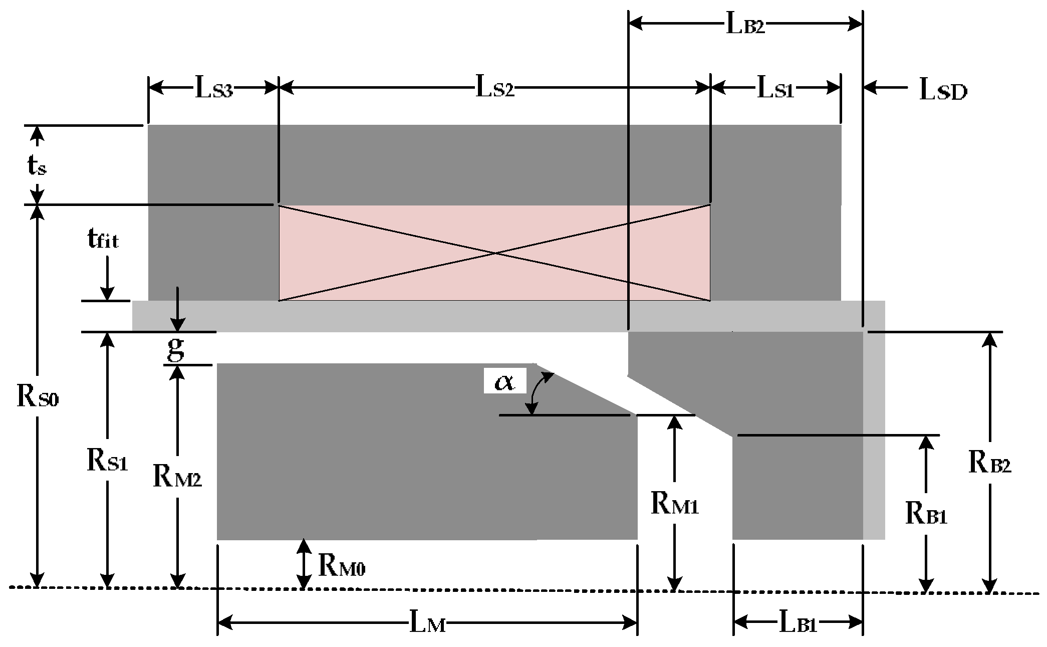
The permeance is the reciprocal of the reluctance (R), and the reluctance physical characteristics are similar to the resistance. Shorter paths or larger cross-sectional areas produce smaller reluctance, easier flow and better permeability of the zone. The permeance is represented by parameters, such as path length and cross-sectional area. In Figure 7a, variable $x$ represents the armature displacement, and the definition of size of proportional electromagnet is shown in Figure 8. The results are shown in

Table 2. Permeance of air gaps in the proportional electromagnet.

Permeance	Mean Path Area	Mean Path Length (${\mathit{l}}_{\mathit{i}}$)	Equation (${\mathit{P}}_{\mathit{A}\mathit{i}}$)
$P_{A1}$	$CFHG$	$x+x_0$	$u{A}_1/l_1$
$P_{A2}$	$DLMN$	$x\sin \alpha$	$u{A}_2/l_2$
$P_{A3}$	$ABCD$	$\sqrt{\overline{{\mathrm{O}}_1\mathrm{D}}\cdot \min (\overline{{\mathrm{O}}_1\mathrm{C}},\overline{{\mathrm{O}}_1\mathrm{X}})}$	$4u_0{P}_{31}{P}_{32}$
$P_{A4}$	$ADN$	—	$3.315u_0(R_{m1}+(\overline{O_{1}D}\cdot \cos \alpha )/2)$
$P_{A5}$	$MPQR$	$\sqrt{\overline{O_{2}M}\cdot \min (\overline{O_{2}R},\overline{O_{2}Y)}}$	$4u_0{P}_{51}{P}_{52}$
$P_{A6}$	$LMP$	—	$3.315u_0[R_{O2}+(\overline{O_{2}M}\cos \alpha )/2]$
$P_{A7}$	—	$g$	$\frac{2\pi u_0}{g}(R_{M2}+\frac{g}{2})\cdot \min (L_{S3},L_{P7})$
$P_{A8}$	—	—	$3.315u_0(R_{M2}+g/2)\cdot K_8$
$P_{A9}$	—	$\sqrt{g\cdot R_{9o}}$	$4u_0(R_{B2}-l_9)\ln \frac{R_{9o}}{g}$

.

2.3. Equivalent Permeance of Air Gaps

The front end equivalent permeance can be obtained after series connection, as shown in Equation (2) and Table 2. It is obtained the same way as the rear end gap, as shown in Equation (3). The proportional electromagnet in this study is designed as a modular configuration, so the non-magnetic material is used to attach the base and the armature acts as a guide tube. Because the permeability coefficient of non-magnetic material is similar to that of air, it is considered in the formula for the air gap zone. The permeance results are shown in Equation (4). The total equivalent permeance of the air gap zone can be calculated using Equations (2)–(4). The series connection is shown in Equation (5).

$$P_{air1}=P_{A1}+P_{A2}+P_{A3}+P_{A4}+P_{A5}+P_{A6}$$

(2)

$$P_{air2}=P_{A7}+P_{A8}+P_{A9}$$

(3)

$$P_{air3}=\frac{\pi u_0(R_{B2}+R_{S1})L_{S1}{L}_{S3}}{(L_{S1}+L_{S3})t_{fit}}$$

(4)

$$P_{air}={(P_{air1}^{-1}+P_{air2}^{-1}+P_{air3}^{-1})}^{-1}$$

(5)

2.4. Permeance of Metal Zone Calculation

As mentioned above, when the proportional electromagnet is energized, it forms a closed magnetic field and the simplified magnetic flux $\left(\mathrm{\Phi }\right)$ path of the metal zone is shown in Figure 9. Areas with different amperage $\left(NI\right)$ will lead to different magnetic field intensity $\left(H\right)$. Furthermore, the magnetomotive force $\left(F_{sum}\right)$ and magnetic flux density $\left(B\right)$ exist within the metal.

The permeability coefficient of metal is a non-constant, so there is a nonlinear correspondence between its H and B. When the magnetic flux density is higher than a specific value, it will lead to magnetic saturation, so the magnetic flux density may not increase even though the magnetic field is strengthened. The magnetic field intensity could be obtained by the correspondence with magnetic flux density through the material B-H curves, and the results are shown in

Table 3. Permeance parameter of metal zone.

$\mathit{i}$	Mean Path Area (${\mathit{A}}_{\mathit{i}}$)	Mean Path Length (${\mathit{l}}_{\mathit{i}}$)	${\mathit{P}}_{\mathit{S}\mathit{i}}$
1	$2\pi t_s{R}_{so}$	$L_{S2}+(L_{S1}+L_{S3})/2$	$u_S{A}_1/l_1$
2	$\pi (R_{si}+R_{so}+t_s/2)\cdot L_{S1}$	$R_{so}+t_s/2$	$u_S{A}_2/l_2$
3	$\pi (R_{B2}+R_{MO})\cdot L_{B1}$	$R_{B2}-(R_{M2}+R_{M0})/2$	$u_S{A}_3/l_3$
4	$\pi (R_{B2}^2-R_{MO}^2)$	$L_{B1}/2$	$u_S{A}_4/l_4$
5	$\pi (R_{M2}^2-R_{MO}^2)$	$L_M$	$u_S{A}_5/l_5$
6	$\pi (R_{si}+R_{so}+t_s/2)\cdot L_{S3}$	$L_{S2}+(L_{S1}+L_{S3})/2$	$u_S{A}_6/l_6$

.

When it is energized, the proportional electromagnet forms a closed magnetic circuit and the inside paths are connected in series. Therefore, the magnetic flux is the same and the magnetomotive force of each metal zone is obtained by magnetic flux multiplied by the reciprocal of permeance. The magnetic flux density of metal material is obtained by calculating the magnetic flux and then corresponding to the magnetic field intensity to allocate the magnetomotive force of metal and air gaps. The equivalent permeance of the metal zone within the proportional electromagnet is shown in Equation (6).

$$P_{steel}=R_{steel}^{-1}={({\displaystyle \sum _{i=1}^6{R}_{Si}})}^{-1}={({\displaystyle \sum _{i=1}^6{P}_{Si}^{-1}})}^{-1}$$

(6)

2.5. Solenoid Force of Proportional Electromagnet

The total permeance of the proportional electromagnet is the reciprocal of the total reluctance, shown in Equation (7). It can be obtained by the series connection of air gaps and metal zones. When magnetomotive force exists, the magnetomotive force of air gaps can be obtained by the permeance and magnetic flux, and it varies with the armature position, as shown in Equation (8). Due to material properties, the magnetomotive force of metal zones is determined by the magnetic field intensity, as shown in Equation (9), although the permeability of steel ($u_{Si}$) cannot be obtained in advance. When the magnetic flux is obtained, the magnetic field intensity corresponds with the B-H curves. Then, the magnetomotive force can be calculated.

$$P_{sum}=R_{sum}^{-1}={[P_{air}^{-1}+P_{steel}^{-1}]}^{-1}=P_{air}{P}_{steel}/(P_{air}+P_{steel})$$

(7)

$$F_{air}=\mathrm{\Phi }{R}_{air}=\mathrm{\Phi }{P_{air}}^{-1}$$

(8)

$$F_{steel}={\displaystyle {\sum }_{j=1}^6{H}_j}{l}_j={\displaystyle {\sum }_{j=1}^6\frac{B_j}{u_{si}}}{l}_j={\displaystyle {\sum }_{j=1}^6\frac{\mathrm{\Phi }}{u_{si}{A}_j}}{l}_j$$

(9)

$$NI=F_{sum}=F_{air}+F_{steel}$$

(10)

In terms of the armature solenoid force, the input energy can be converted into magnetic energy and mechanical energy according to the conservation of energy, as shown in Equation (11). The current and the metal permeance are unrelated to armature displacement. When the stable current is input, the differential value of some items is zero. It can be derived from the principle of virtual work ($W$). The armature thrust can be obtained by the magnetic flux and permeance of gap zones and its derivation, as shown in Equation (12). A negative sign indicates the opposite direction of displacement force.

$$W=\frac{1}{2}{\mathrm{\Phi }}^2{R}_{air}=\frac{1}{2}{\mathrm{\Phi }}^2{P_{air}}^{-1}$$

(11)

$$\begin{array}{ll}{F}_{em}& =\frac{\partial W}{\partial x}=-\frac{{\mathrm{\Phi }}^2}{2}\cdot \frac{d}{dx}(P_{air1}^{-1}+P_{air2}^{-1}+P_{air3}^{-1})\\ & =-\frac{{\mathrm{\Phi }}^2}{2}\cdot [P_{air1}^{-2}\frac{d}{dx}{P}_{air1}+P_{air2}^{-2}\frac{d}{dx}{P}_{air2}+P_{air3}^{-2}\frac{d}{dx}{P}_{air3}]\end{array}$$

(12)

As mentioned above, the armature solenoid force can be obtained by the magnetic flux and air gap parameter of Equations (2)–(4). The magnetic flux is an unknown input parameter since it has a nonlinear relationship with the input current, and it is obtained by the calculation program. The database of magnetic flux and magnetomotive force should be created, the actual magnetic flux is obtained through the input current. Then, the proportional solenoid force, as derived from Equation (11), is entered into Equation (12).

3. Design and Simulation of Solenoid Force

3.1. Configuration Parameter Design

After the excitation of two materials, mutual attraction is generated and the attraction may be greatly attenuated with the separation distance. The reluctance of air gap is reduced when the two materials are close to each other, as shown in Equation (12). Most air gap reluctance increases with armature away from the base, but $P_{A3}$ is the opposite. In a particular path, the total reluctance of the proportional electromagnet is constant, so that the armature thrust must remain stable and would not change with the displacement.

Therefore, the design of parameters needs to focus on the permeance change of $P_{A3}$ and $P_{A1}$. Considering the collocation with each other, the optimized configuration of proportional electromagnet was completed. The following is a brief description of how some important parameters influence the electromagnetic force.

3.1.1. Base Flange

The base flange ($L_{B2}-L_{B1}$) mainly influences the parameters of the front end air gap. A shorter cone zone gives better permeance of air gap, and the permeability also increases. Therefore, the solenoid force is enhanced, and the horizontal becomes worse. The configuration boils down to the general electromagnet when there is no cone zone. The design is generally determined by the working stroke, so the stroke of the proportional valve must be within 1 mm. To avoid a strong magnetic attraction starting zone, a dimension of 1.5 mm for the product finally was taken as the design value. The simulation results are shown in Figure 10.

3.1.2. Taper Angle

With the taper angle ($\alpha$), the size of configuration greatly influences the permeance of the front end air gap, and it is the most important parameter determining the electromagnetic force. When the taper angle decreases, $P_{A2}$ and $P_{A4}$ may relatively increase, and $P_{A3}$ changes with it. Therefore, the angle is reduced and the electromagnetic force clearly increases away from the armature (the trend of change is determined according to the rate of change of parameters $P_{31}$ and $P_{32}$). Using a wide angle can achieve a better horizontal dimension of the control zone, but the electromagnetic force is relatively weak. Finally, seven degrees was adopted as the design value for the product size, and simulation results are shown in Figure 11.

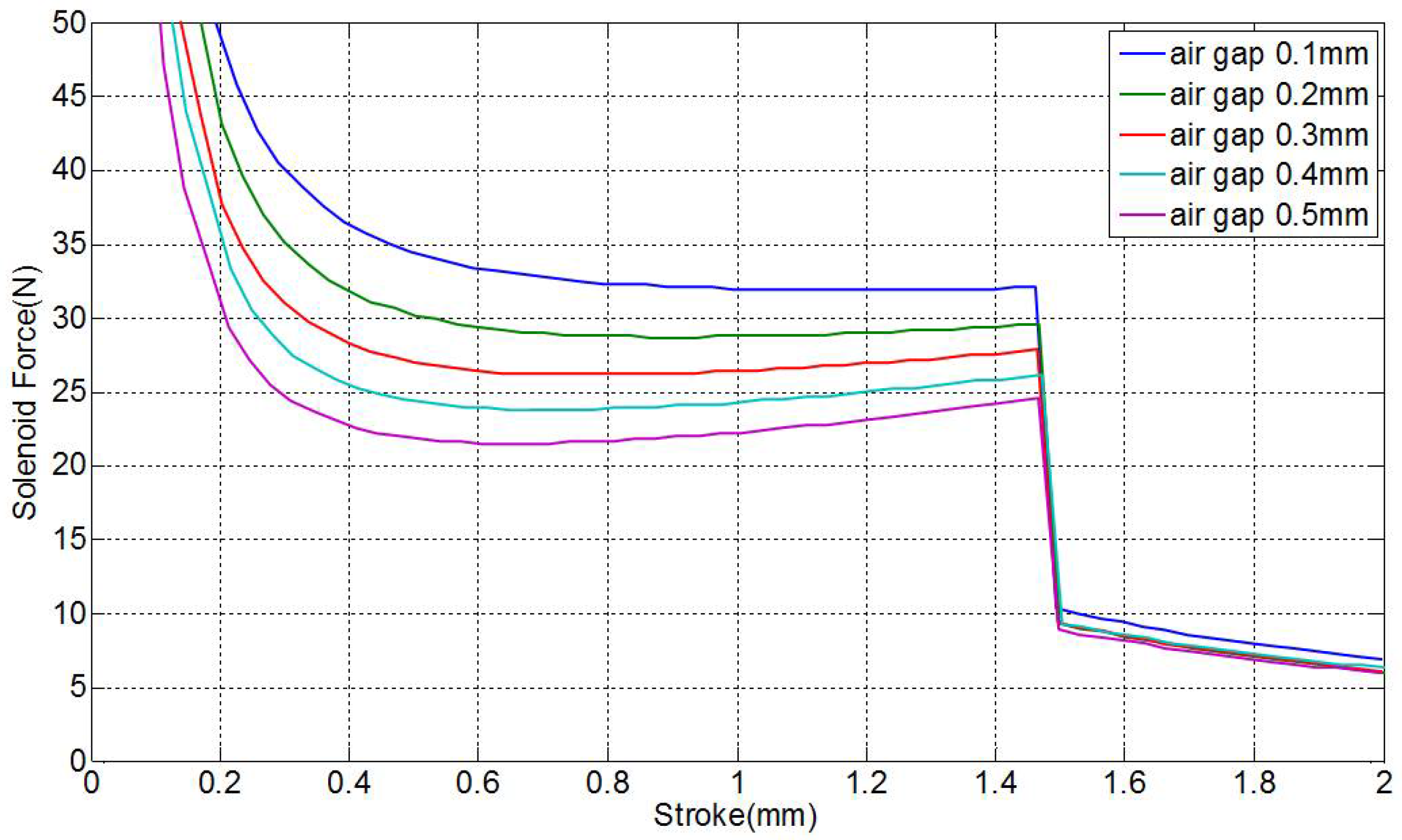
3.1.3. Air Gap

To achieve a small volume but large thrust, the combination is better with smaller gap, thinner guide tube of proportional electromagnet, and smaller air gap between armature and base. Considering the actual needs of processing, the assembly was given a 0.1 mm air gap ($g$), 0.35 mm of guide tube ($t_{fit}$), and 0.1 mm of unilateral radius difference ($R_{M1}-R_{B1}$) between armature and base. The simulation results are shown in Figure 12 and Figure 13.

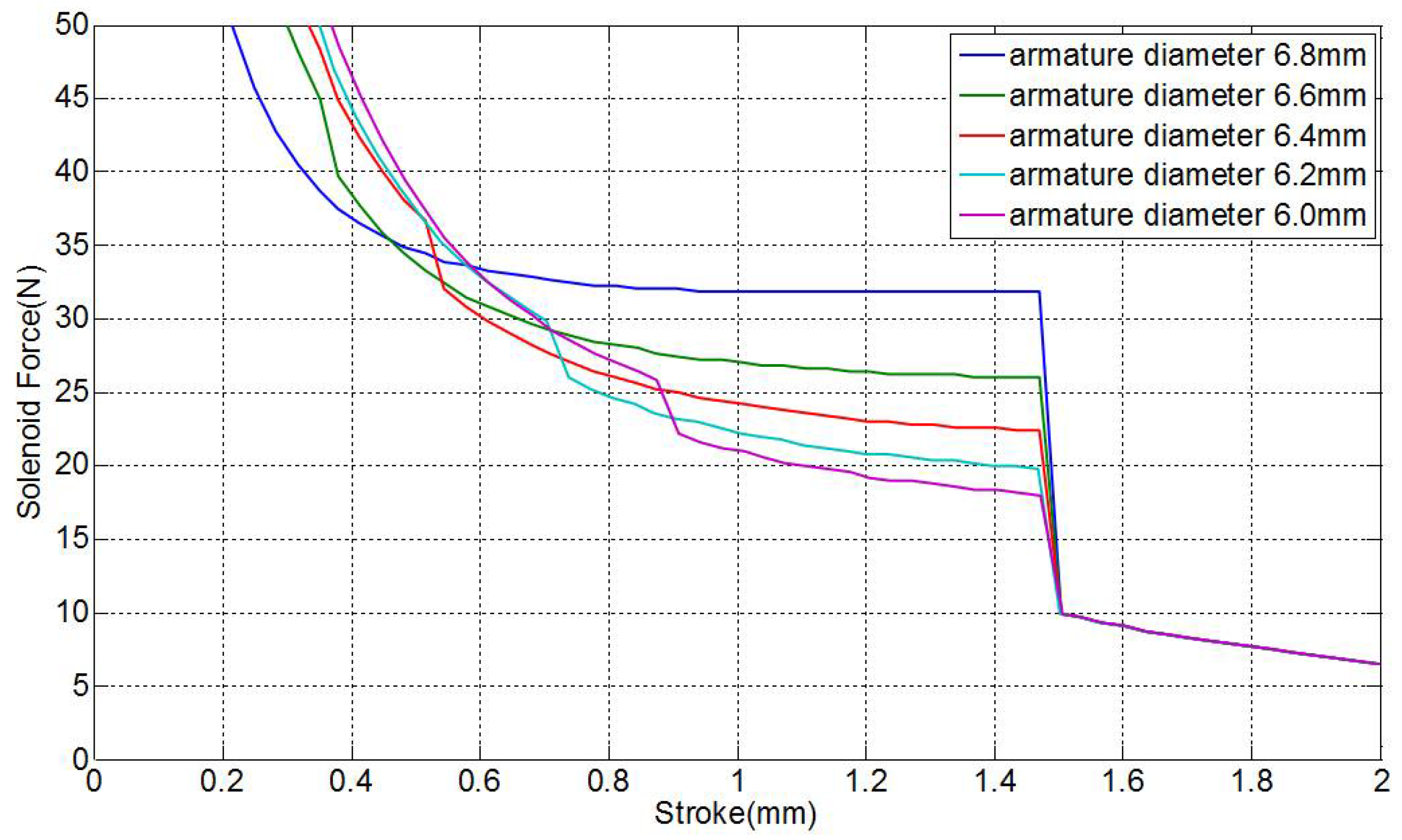
For the simulation parameters, the gap between armature and base bottom diameter is the critical dimension because it directly affects the characteristic of thrust curve. When the difference between armature and base is close to zero, it can achieve better performance. To prevent the armature diameter from being bigger than the base and then generating interference, a diameter of 6.8 mm for the armature was used in the final design. The displacement cannot influence the guide tube thickness and assembly air gap, so the thrust curve will not change. The simulation results are shown in Figure 14.

3.1.4. Parameter Design Results

Through the analysis of simulation results, detailed parameters such as base flange, taper angle, guide tube, air gap, and armature diameter were determined to obtain smooth, long-stroke, and large-thrust horizontal control zone. The relevant parameters are summarized and compared in

Table 4. The relevant parameters are summarized and compared.

	Feature	Location (Figure 8)	Design Size	Thrust (N)	Size V.S. Thrust
Parameter
base flange		$L_{B2}-L_{B1}$	1.5 mm	31	Size ↑, Thrust ↓
taper angle		α	70	31	Angle ↑, Thrust ↑
guide tube		$t_{fit}$	0.35 mm	31	Size ↑, Thrust ↓
air gap		$g$	0.1 mm	32	Size ↑, Thrust ↓
armature diameter		$R_{M2}-R_{M0}$	6.8 mm	32	Size ↑, Thrust ↑

.

3.2. Simulation and Test Results of Armature Force

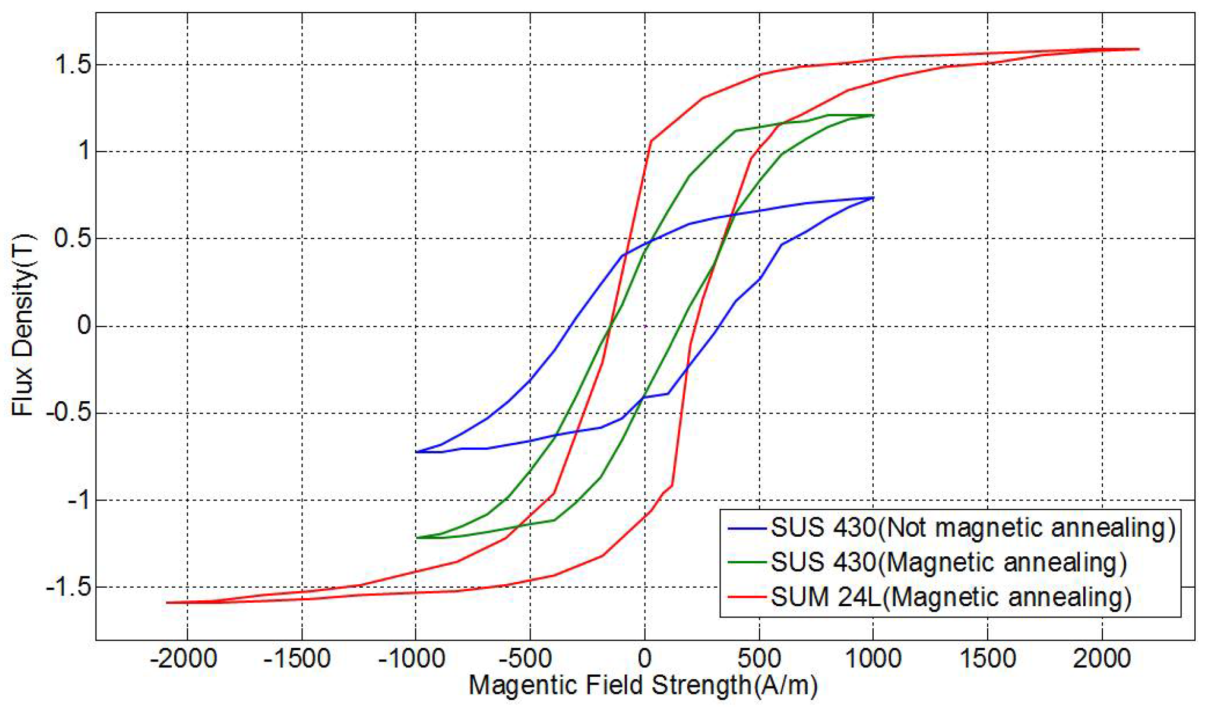
Using three different armature materials for the electromagnet and armature material, hysteresis tests are shown in Figure 15. After magnetic annealing, materials have a higher B-H. SUS 430 steel is easier to achieve magnetic saturation, and SUM 24L steel has higher magnetic flux (large slope). Thus, SUM 24L steel has a higher thrust curve and is suitable for the proportional electromagnet material.

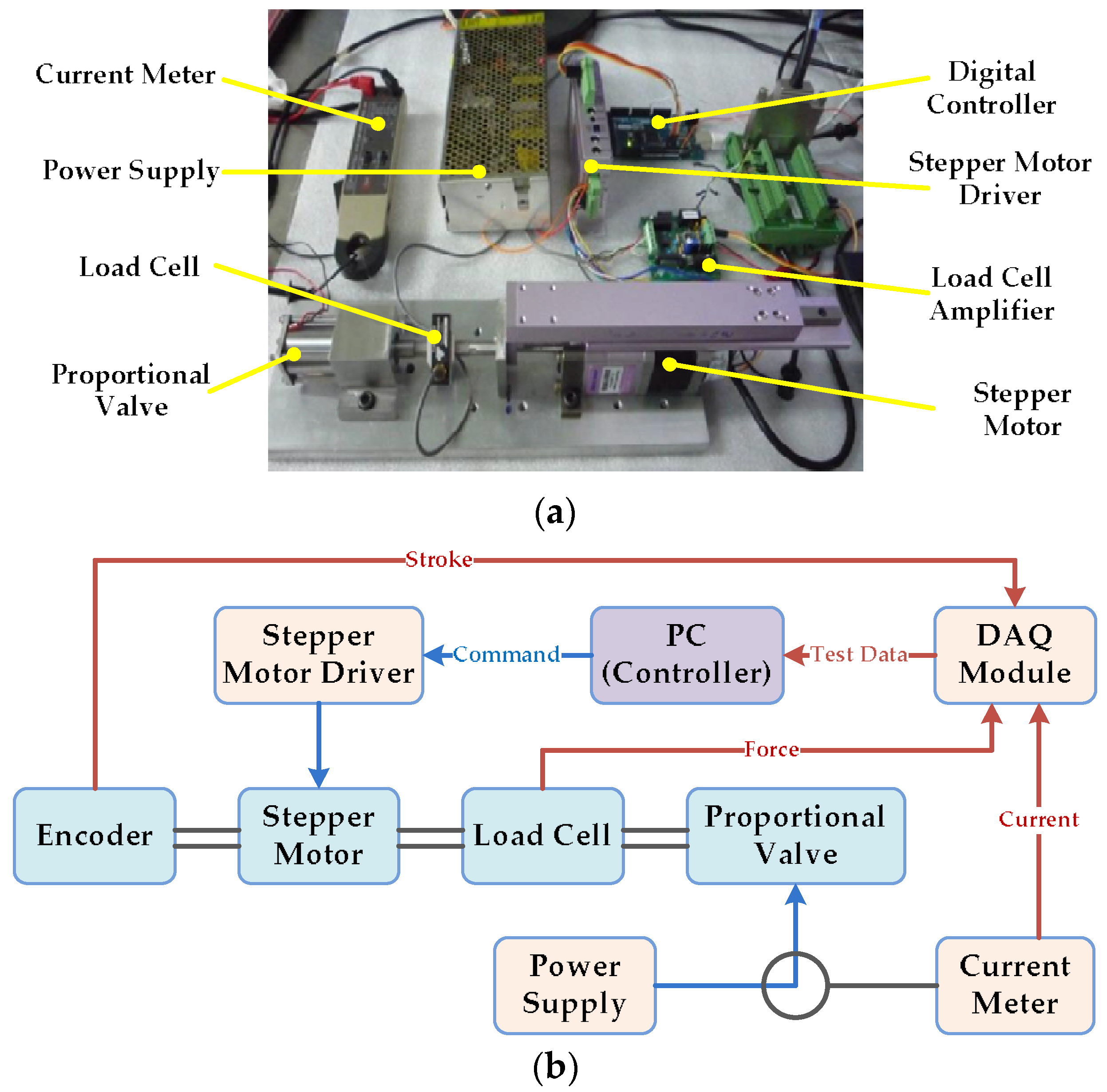
Figure 16 shows the configuration of the proportional valve solenoid force test. The PC-based control unit is composed of the experimental software, a load cell, a digital controller, a steeper motor, and a proportional valve. Thus, the stepping motor pulls the proportional valve inside the armature to move, and the relationship between the solenoid force and the stroke of the armature at different voltages (8 V, 10 V, and 12 V) can be observed.

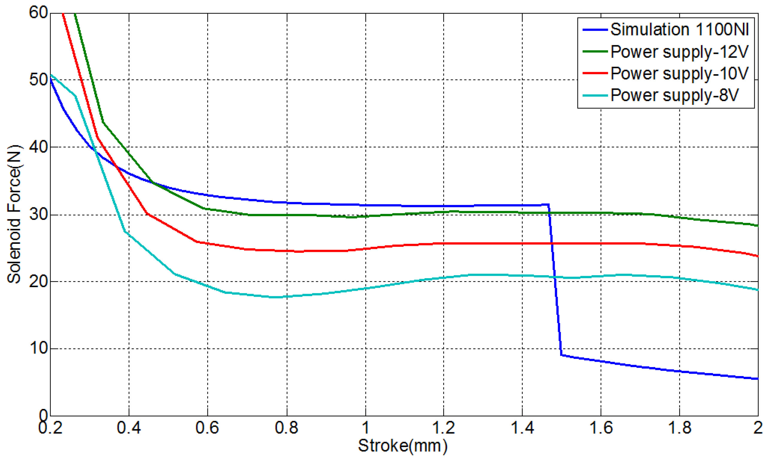
Figure 17 shows solenoid force simulation and test results. The solenoid force is proportional to the linear relationship by using SUM 24L steel (magnetic annealing) for the armature, magnetic base, and three different input voltages. The solenoid force required for the proportional valve is 30 N. When 12 V voltages is input, the horizontal control zone can reach 30 N for achieving the expected full pressure relief function. However, when the stroke is over 1.5 mm, the force is not completely decreased rapidly and the simulation value is different. It is possible that the test results were influenced by an electromagnetic leakage, and the future control zone should be set at a stroke from 0.7 mm to 1.5 mm to avoid non-horizontal control zone.

4. Design and Test of Proportional Valve

4.1. Design of the Proportional Valve Body

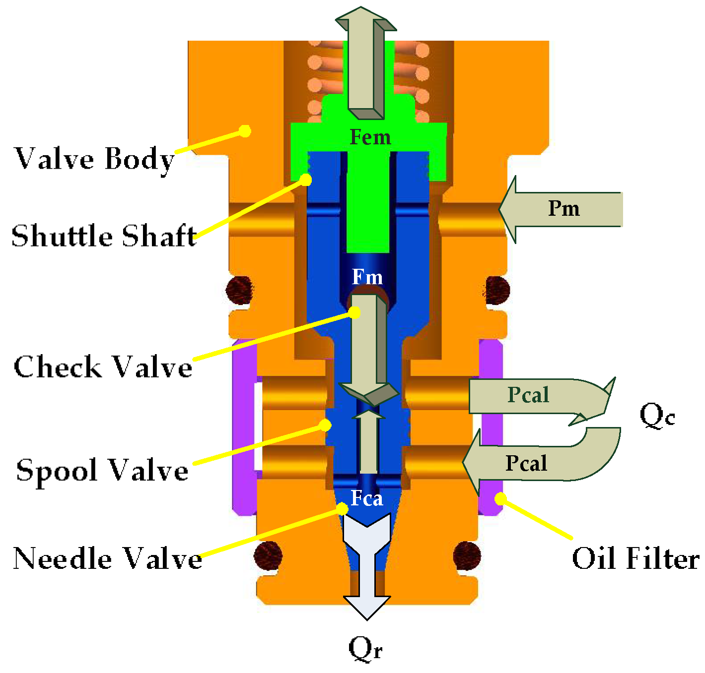
A proportional pressure control valve is composed of the proportional electromagnet set and valve body set, which comprises a magnetic armature, spool valve, housing, and needle valve seat. The design is shown in Figure 18. The outlet and inlet $P_{cal}$ are connected, and they both have connection calipers. Although the valve body has four ports, it is three-port and two-position structure.

Through the shuttle shaft operation, the needle valve port must be closed, and it allows no internal leakage when there is no actuation. With the cone design, the check valve within the shuttle shaft is a safety device. If the needle valve malfunctions, the shuttle shaft cannot be returned to the original position, but the caliper pressure can still be relieved through the check valve. If the spring pre-pressuring is ignored, the shuttle shaft force equation is as follows:

$$F_m=F_{em}+F_{cal}$$

(13)

In addition $F_m=P_m\ast A_{sp}$, $F_{cal}=P_{cal}\ast (A_{sp}-A_{ol})$.

Substituting Equation (13),

$$P_{cal}=(F_m-F_{em})/(A_{sp}-A_{ol})$$

(14)

Where $F_m$ is the master cylinder pressure acting on the shuttle shaft force; $F_{em}$ is the proportional solenoid force; $F_{cal}$ is the caliper chamber pressure acting on the shuttle shaft force;$P_m$ is the master cylinder pressure; $P_{cal}$ is the caliper pressure; $A_{sp}$ is the spool valve cross-sectional area; and $A_{ol}$ is the needle valve hole cross-sectional area.

Assuming that the master cylinder pressure ($P_m$) is 172 bars, the general ABS specifications must reduce the calipers pressure ($P_{cal}$) to 69 bars or less. The spool shaft diameter is 1.8 mm, the proportional solenoid force is about 3.0 kgf, and the needle valve hole and calipers hole are 0.6 mm. The spool valve is fully closed when it moves 0.6 mm. Then, substituting values into Equation (14), the pressure relief value is calculated and the design meets requirements.

Regarding the rated flow calculation [17], the master cylinder pressure must remain constant. The pressure $P_c$ which is flowing through the spool valve is the supply pressure for the brake calipers with flow rate $Q_c$. The valve orifice area $A_c$ may vary with the displacement changes of shuttle shaft. Pressure $P_r$ flows through the needle valve with flow rate $Q_r$, and the needle valve orifice area is $A_r$. The equation which the spool valve port and the needle valve port flow through is as follows.

$$P_{cal}=\frac{(\frac{172\ast \pi \ast {0.18}^2}{4}-3.0)}{\frac{\pi }{4}({0.18}^2-{0.06}^2)}=60.8bars$$

$$Q_c=C_d{A}_c\sqrt{\frac{2(P_m-P_c)}{\rho }}$$

(15)

$$Q_r=C_d{A}_r\sqrt{\frac{2(P_c-P_r)}{\rho }}$$

(16)

The opening size of spool valve port and needle valve port are in a relation of mutual growth and decline. The maximum flow rate probably occurs when the two vale ports are in half-open position, which means the stroke is in the 0.3 mm position. The relationship of pressure is $P_m-P_c=P_c-P_r$ and $P_r$ is close to zero. Thus, $P_c$ is approximately a half of $P_m$. In the steady state, $Q_c=Q_r$, the maximum flow rate could be obtained by estimating the flow of spool valve. The half-open cross-sectional area of spool valve is as follows.

$$A_c=\frac{1}{2}(\frac{\pi {(0.06)}^2}{4})=0.001413{\mathrm{cm}}^2$$

Substituting Equation (15),

$$\begin{array}{c}{Q}_c=0.7\ast 0.001413\ast 100\ast \sqrt{\frac{2\ast (172-86)\ast {10}^5}{1000}}\\ =13{\mathrm{cm}}^3/\sec =0.78l/\min \end{array}$$

4.2. Single Proportional Valve Test

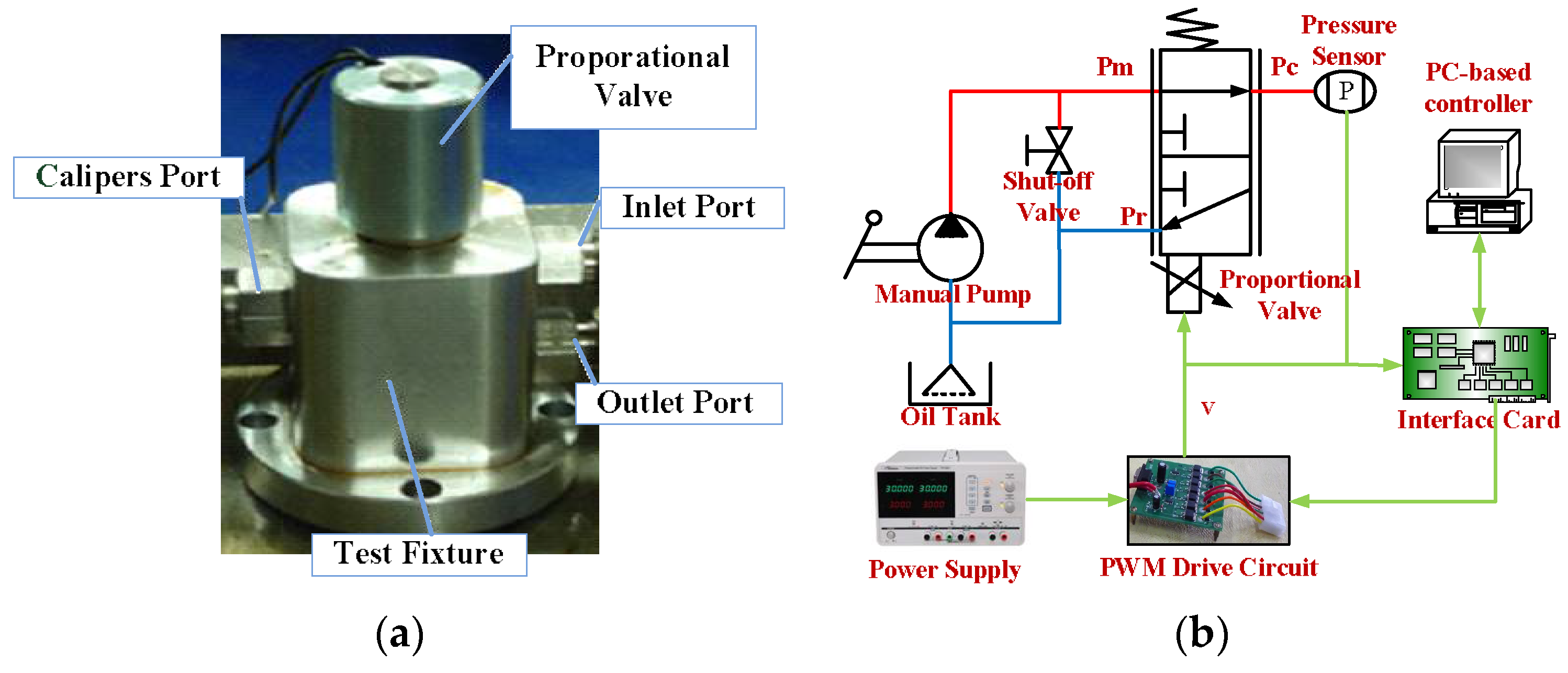
This test is to confirm that the proportional solenoid energy is powerful enough to achieve the desired pressure relief of the proportional valve and that it could be used to control the brake calipers. When the input voltage is different, the armature can obtain a corresponding magnetic attraction and then drive the valve port to open. The single proportional valve test rig is shown in Figure 19a. To confirm the ability of relief, the high pressure of input port is compared with the pressure on the caliper port.

The experimental procedure of the proportional valve system is described and shown in Figure 19b. The system circuit is pressurized to 175 bars with a hand pump. The PC-based control unit includes an experimental software program, a pressure sensor, an AD/DA interface card and a PWM drive circuit. The control signals are computed in the PC-based control unit, and that drives the proportional valve via an AD/DA interface card and a PWM drive circuit with the sampling time of 1 ms. Thus, the solenoid force pulls the proportional valve inside the armature to move and the relationship between the command and the pressure on the calipers port at preloading (175 bars). The testing order is mainly step wave and triangular wave command-based since the step wave could confirm the reaction time, and the triangle wave could confirm the follow state and linearity.

To verify the pressure relief performance of proportional valves, the single proportional valve must be tested to confirm the pressure relief function and facilitate the ABS wheel configuration design. Because the braking force is related to the brake pedal or handle brake of drivers, the caliper chamber pressure at each brake condition is tested with dissimilar initial pressures. In addition, the proportional solenoid is applied with 10 V to drive the single proportional valve for the maximum pressure relief test.

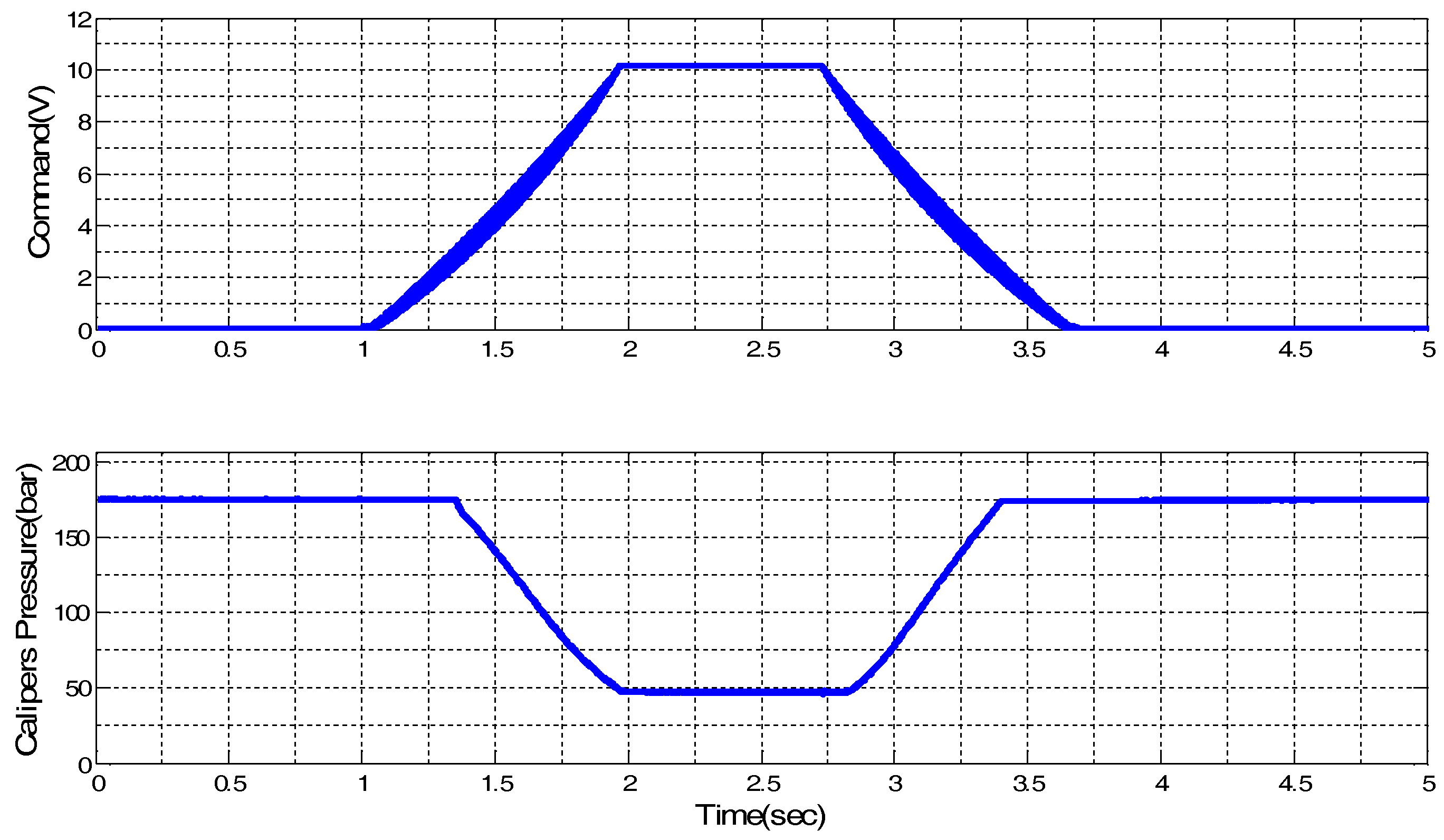
Figure 20 shows the triangular wave command relief test results. When the power supplies 12 V (vehicle voltage), the proportional solenoid is not actuated at command 2.5 V or less, and the pressure drop is 130 bars above 10 V. The pressure drop between 2.5 V to 10 V is linear, and the relationship between voltage and pressure drop can be derived as 17.3 bars/V. The caliper pressure follows the command well and linearly, and the pressure does not have vibration when the valve is fully open. The solenoid force calculated as a result of the experiment is as follows:

$$\frac{(\frac{175\ast \pi \ast {0.18}^2}{4}-F_{em})}{\frac{\pi }{4}({0.18}^2-{0.06}^2)}=45\mathrm{bars}\Rightarrow F_{em}=33.6N$$

The calculated test result is greater than the simulated value (30 N).

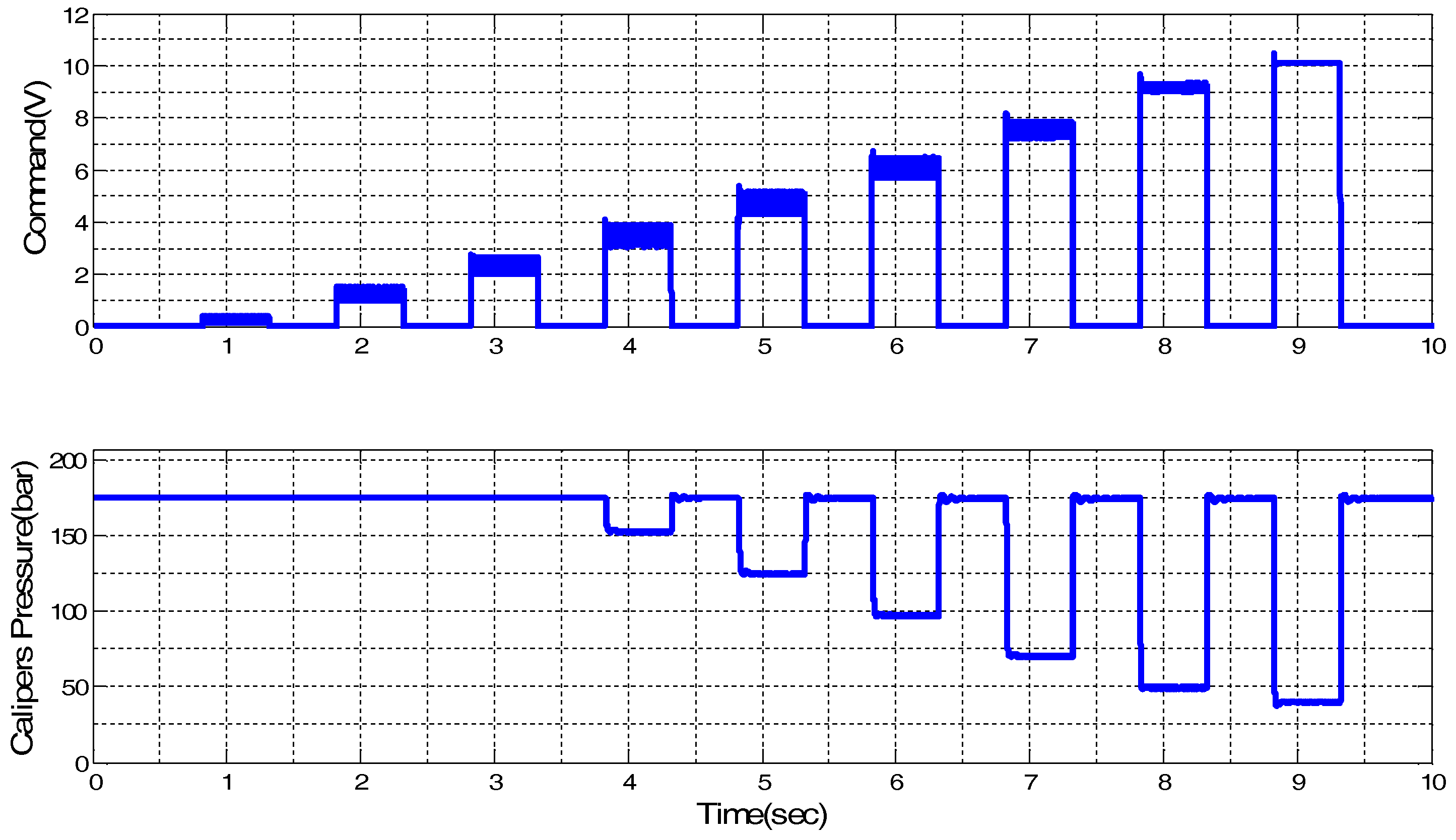
Figure 21 shows step wave command relief test results. It shows that when the voltage is lower than 3 V, the electromagnetic force is insufficient to open the valve port. The corresponding pressure drops for 3, 4.5, 6, 7.5, 9, and 10 V are, respectively, 25, 50, 75, 105, 125, and 130 bars. Figure 22 shows the time response when the step wave command is 10 V. The valve opening time is 9 ms (timing sequence from 8.821 s to 8.3 s) and the valve closing time is 5 ms (timing sequence from 9.321 s to 9.326 s). This proportional valve test meets with application requirements, and it can be used as a reference for the internal controller of the subsequent ABS module as the basis for the slip control calculation.

5. Conclusions

This study aimed to integrate the Inlet Valve (Inlet Valve normally open) and Outlet Valve (Outlet Valve normally closed) of an EHB, which has the same function as a three-port, two-position braking proportional pressure control valve. The assembly was composed of a cone lift lever (with electromagnet), the valve shell case, a valve body (including the top plug seats), and the proportional solenoid coil.

This new product development was tested under simulated braking force of pressing 175 bars, and its pressure drop is up to 130 bars. In terms of electromagnetic force, it can reach more than 30 N. Thus, this product can meet the demand of an ABS wheel anti-lock pressure relief and pressure relief adjustment control. Moreover, it provides ABS closed-loop control and has good linear control accuracy and repeatability. Overall, this product meets the design requirements.

References

- Aksjonov, A.; Augsburg, K.; Vodovozov, V. Design and Simulation of the Robust ABS and ESP Fuzzy Logic Controller on the Complex Braking Maneuvers. Appl. Sci. 2016, 6, 382. [Google Scholar] [CrossRef]
- Ivanov, V.; Savitski, D.; Augsburg, K.; Barber, P.; Knauder, B.; Zehetner, J. Wheel slip control for all-wheel drive electric vehicle with compensation of road disturbances. J. Terramech. 2015, 61, 1–10. [Google Scholar] [CrossRef]
- Mirzaei, M.; Mirzaeinejad, H. Optimal design of a non-linear controller for anti-lock braking system. Transp. Res. Part C 2012, 24, 19–35. [Google Scholar] [CrossRef]
- Mirzaeinejad, H.; Mirzaei, M. A novel method for non-linear control of wheel slip in anti-lock braking systems. Control Eng. Pract. 2010, 18, 918–926. [Google Scholar] [CrossRef]
- Wang, B.; Huang, X.; Wang, J.; Guo, X.; Zhu, X. A robust wheel slip ratio control design combining hydraulic and regenerative braking systems for in-wheel-motors-driven electric Vehicles. J. Frankl. Inst. 2015, 352, 577–602. [Google Scholar] [CrossRef]
- Wu, M.C.; Shih, M.C. Simulated and experimental study of hydraulic anti-lock braking system using sliding-mode PWM control. Mechatronics 2003, 13, 331–351. [Google Scholar] [CrossRef]
- Qiuetal, Y.; Liang, X.; Dai, Z. Backstepping dynamic surface control for an anti-skid braking system. Control Eng. Pract. 2015, 42, 140–152. [Google Scholar]
- Tanelli, M.; Sartori, R.; Savaresi, S.M. Combining Slip and Deceleration Control for Brake-by-wire Control Systems: A Sliding-mode Approach. Eur. J. Control 2007, 6, 593–611. [Google Scholar] [CrossRef]
- Lv, C.; Zhang, J.; Li, Y.; Yuan, Y. Novel control algorithm of braking energy regeneration system for an electric vehicle during safety-critical driving maneuvers. Energy Convers. Manag. 2015, 106, 520–529. [Google Scholar] [CrossRef]
- Patra, N.; Datta, K. Observer based road-tire friction estimation for slip control of braking system. Procedia Eng. 2012, 38, 1566–1574. [Google Scholar] [CrossRef]
- Bhandari, R.; Patil, S.; Singh, R.K. Surface prediction and control algorithms for anti-lock brake system. Transp. Res. Part C 2012, 21, 181–195. [Google Scholar] [CrossRef]
- Choa, J.R.; Choia, J.H.; Yoo, W.S.; Kim, G.J.; Woo, J.S. Estimation of dry road braking distance considering frictional energy of patterned tires. Finite Elem. Anal. Des. 2006, 42, 1248–1257. [Google Scholar] [CrossRef]
- Chen, C.P.; Tung, C.; Chen, C.A. A Proportional Electro-Hydraulic Breaking Control Valve, Taiwan, 2010. Patent No. I320374, 11 February 2010. [Google Scholar]
- Lee, C.O.; Song, C.S. Analysis of the solenoid of a hydraulic proportional compound valve. In Proceedings of the 35th National Conference on Fluid, Chicago, IL, USA, 13–15 November 1979. [Google Scholar]
- Chen, Y.N.; Kuo, W.H. Analysis and Design of Proportional Pressure Control Valve. Master’s Thesis, National Taiwan University, Taipei, Taiwan, 1987. [Google Scholar]
- Chen, C.A.; Tung, C.; Chen, C.P. The Proportional Solenoid Module for a Hydraulic System, Taiwan, 2015. Patent No. I474350, 21 February 2015. [Google Scholar]
- Merritt, H.E. Hydraulic Control Systems, 3rd ed.; John Wiley & Sons: Hoboken, NJ, USA, 1985; pp. 76–113. [Google Scholar]
Figure 1.
Hydraulic circuit of EHB actuator between master cylinder and wheel cylinder.
Figure 2.
Relationship between wheels and pavement.
Figure 3.
Proposed hydraulic circuit with a PEHB actuator.
Figure 4.
Configuration of proportional pressure control valve for PEHB actuator.
Figure 5.
Relation between solenoid force and stroke: (a) form of force; and (b) flux path mode.
Figure 6.
Simplification of the six types of magnetic path.
Figure 7.
Air gaps magnetic flux path: (a–c) front end; and (d) rear end.
Figure 8.
Definition of size for the proportional electromagnet.
Figure 9.
Magnetic flux path of the metal zone.
Figure 10.
Simulation results of base flange.
Figure 11.
Simulation results for the taper angle.
Figure 12.
Simulation results for the guide tube.
Figure 13.
Simulation results for the air gap.
Figure 14.
Simulation results for the armature diameter.
Figure 15.
B-H curves of material.
Figure 16.
Configuration of the proportional valve solenoid force test: (a) test rig; and (b) structure.
Figure 17.
Simulation and test results for the proportional valve solenoid force.
Figure 18.
Proportional valve body construction and fluid force.
Figure 19.
Configuration of single proportional valve test: (a) test rig; and (b) structure.
Figure 20.
Triangular wave command at proportional valve relief test in 175 bars.
Figure 21.
Step wave command at proportional valve relief test in 175 bars.
Figure 22.
Step wave command at proportional valve relief test in 175 bars (timing sequence from 8.6 s to 9.6 s).