Model Predictive Stabilization Control of High-Speed Autonomous Ground Vehicles Considering the Effect of Road Topography

Featured Application

This work presents an MPC scheme for stabilization control of high-speed autonomous ground vehicles (AGVs) considering the effect of road topography. Accounting for the road curvature and bank angle, this scheme is able to maintain handling stability by preventing excessive sideslip and rollover while ensuring collision-free trajectories. Such an MPC scheme can not only contribute to the performance of AGVs, but also be used as an advanced safety technique in advanced driver-assistance systems (ADAS) and intelligent transportation systems (ITS).

Abstract

This paper presents a model predictive control (MPC) scheme for the stabilization of high-speed autonomous ground vehicles (AGVs) considering the effect of road topography. Accounting for the road curvature and bank angle, a single-track dynamic model with roll dynamics is derived. Variable time steps are utilized for vehicle model discretization, enabling collision avoidance in the long-term without compromising the prediction accuracy in the near-term. Accordingly, safe driving constraints including the sideslip envelope, zero-moment-point and lateral safety corridor are developed to handle stability and obstacle avoidance. Taking these constraints into account, an MPC problem is formulated and solved at each step to determine the optimal steering control commands. Moreover, feedback corrections are integrated into the MPC to compensate the unmodeled dynamics and parameter uncertainties. Comparative simulations validate the capability and real-time ability of the proposed control scheme.

1. Introduction

As autonomous ground vehicles (AGVs) find increasing utility in both military and commercial applications, driving safety has become a critical issue that impedes their further development [1]. Typically, driving safety is deemed as being collision-free, which may be adequate for earlier applications such as small robots and low-speed vehicles [2,3]. However, since recent research efforts have targeted large-size and high-speed AGVs, the handling stability-related concerns, such as excessive sideslip and rollover, become increasingly important. Inappropriate handling of these dynamics, particularly under a complex road topography, will lead to loss of control of the AGVs or even fatal accidents. Therefore, it is necessary to develop a control scheme that can systematically utilize the knowledge of vehicle dynamics and the road topography information to avoid collisions while ensuring the handling stability of high-speed AGVs.

Recent work has shown that model predictive control (MPC) can be used to rigorously handle the vehicle dynamics and multiple safety constraints [4,5]. Many MPC-based methods have demonstrated successful applications in the field of path following [6], obstacle avoidance [7], emergency maneuvering [8], lane change maneuvers [9], etc. Although these methods do provide good results in their own respective applications, they usually assume simple road topography, i.e., neglecting the road curvature and bank angle. Moreover, most of these applications do not take handling stability-related concerns into account. Instead, they rely on the built-in production systems, such as dynamic stability control (DSC) or electronic stability control (ESC), which enforce stabilization criteria regardless of an impending collision. Thus, while these applications may maintain the stabilization of AGVs, there is no guarantee that the trajectories modified by these built-in systems would be collision-free.

Rather than relying on production systems, alternative approaches have explicitly incorporated stabilization criteria in the MPC formulations for the purpose of vehicle stabilization [10]. Among them, envelope control has been widely applied in the automotive field, and a number of stability envelopes have been developed. Earlier analyses of vehicle handling are presented by defining a stable region with respect to the vehicle sideslip and sideslip rate in the phase plane. The open region between the saddle points of this phase plane is used as a safe envelope for vehicle stability [11,12]. Focusing on limiting the saturation of the tires to prevent loss of control, a vehicle stabilization envelope is proposed to limit the peak forces of the front and rear wheels [13]. Building upon these work, Beal and Gerdes presented a stable handling envelope that combines the phase plane design approach and the explicit consideration of rear tire saturation [14]. This envelope bounds the yaw rate of the vehicle while limiting the rear tire forces below their peak to prevent rear tire saturation. Vehicle sideslip and yaw rate serve as the phase plane variables that capture this stability envelope. Moreover, Gerdes also presented a closed envelope in the sideslip and yaw rate phase plane using isolines [15]. This envelope can incorporate more naturally stable regions of the phase plane in vehicles with strong under-steering characteristics. Recent applications of vehicle stability control enforce constraints only on the maximum allowable rear tire force [16,17].

By virtue of the stability envelope, a continuously-resolved optimization seeking to minimize trajectory tracking errors while satisfying the stabilization criteria is realized. However, this still suffers from the underlying challenge that such constraints may be overly restrictive or conflict with each other, which may lead to tracking errors that result in collisions. Addressing this problem, [18,19] presented a novel method to weight these sometimes conflicting objectives by prioritizing collision avoidance and adding slack variables to hard constraints. If necessary, they even allow the violation of the stabilization criteria temporarily to avoid collisions. Nevertheless, most of these methods neglect the roll dynamics of AGVs and the effects of road topography, which are not always feasible [20]. For example, it is important to account for the roll dynamics when handling an AGV with a high center of gravity (CoG) or driving on a road with a large path curvature and road banks.

Nowadays, many studies accounting for the roll dynamics have been published [21,22]. Many vehicle roll stability metrics, such as the static stability factor (SSF) [23], stability moment (SM) [24], load transfer ratio (LTR) [25], time-to-rollover (TTR) [26], zero-moment-point (ZMP) [27], etc., have also been discussed. While these metrics do provide important results under certain conditions, they are limited by their inherent assumptions. Static metrics such as the SSF are easy to calculate, but do not capture vehicle behavior during dynamic maneuvers. Meanwhile, dynamic metrics such as the LTR and SM rely on information that is difficult to obtain [28]. Metrics using state prediction models, such as the TTR, do not account for the road topography, which significantly affects a vehicle’s rollover propensity. Of all the metrics mentioned above, ZMP is preferable due to its ability to explicitly account for the effects of road topography in its derivation [29]. Moreover, the ZMP can be expressed as a linear combination of the vehicle states, allowing it to be included as an output of any vehicle model.

In this work, we present a novel MPC scheme for stabilization control of high-speed autonomous ground vehicles considering the effects of road topography. Accounting for the effect of path curvature and the road bank, a single-track vehicle model with roll dynamics is derived. To enable collision avoidance in the long-term without compromising the prediction accuracy in the near-term, variable time steps are employed for model discretization. Then, the handling of the stability collision avoidance-related constraints is expressed as the sideslip envelope, limits on ZMP and lateral safety corridor. Accordingly, an MPC problem with feedback corrections is formulated and solved to ensure optimal vehicle operation within these safe driving constraints. Simulations carried out in the MATLAB/CarSim environment validated the effectiveness and real-time ability of the proposed scheme.

2. Preliminaries of MPC and Framework Overview

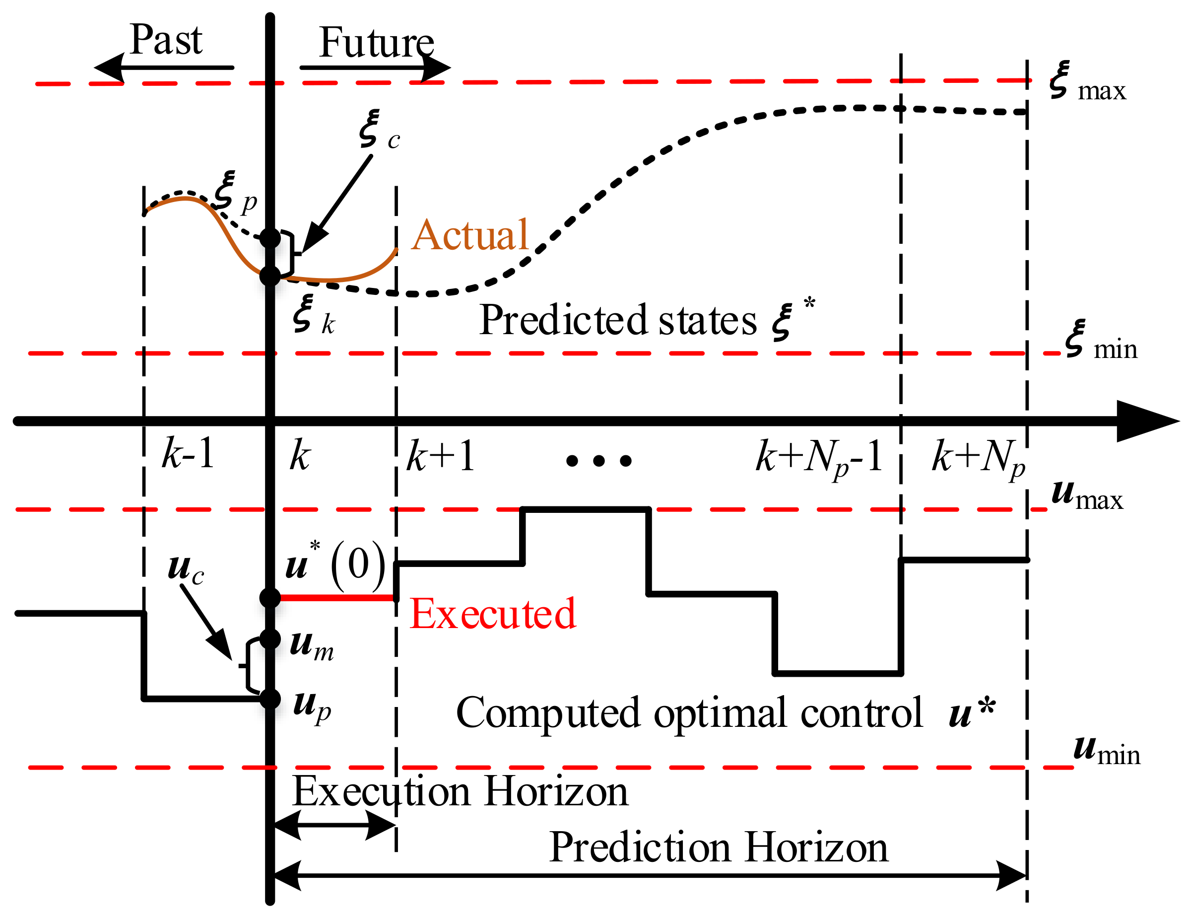
2.1. Preliminaries of MPC

MPC is realized through an iterative on-line optimization over a moving finite prediction horizon, as illustrated in Figure 1. At time step k, starting from the state ${\xi }_k$, an optimal control sequence $u^{\ast }(k+i)$, $i\in [0,N_p-1]$ is computed by solving an open-loop, constrained, finite-time optimal control problem over the prediction horizon $N_p$. The optimal control sequence $u^{\ast }$ is bounded by the input saturations $u_{max}$ and $u_{min}$, and the resulting predicted states ${\xi }^{\ast }$ satisfy the state constraints ${\xi }_{max}$ and ${\xi }_{min}$. Although the optimal control sequence is calculated over the prediction horizon $N_p$, only the first step of that, $u^{\ast }(0)$, is executed.

Due to unmodeled dynamics, parameter uncertainties and/or external disturbances, the measured control action $u_m$ and vehicle state ${\xi }_k$ are highly likely to be different from the predicted value of those obtained from the previous loop, $u_p$ and ${\xi }_p$. The differences between them are denoted as $u_c$ and ${\xi }_c$. In the next step, the optimal control problem is resolved over a shifted horizon based on new measurements. This process is repeated at each step until the terminal requirements are satisfied.

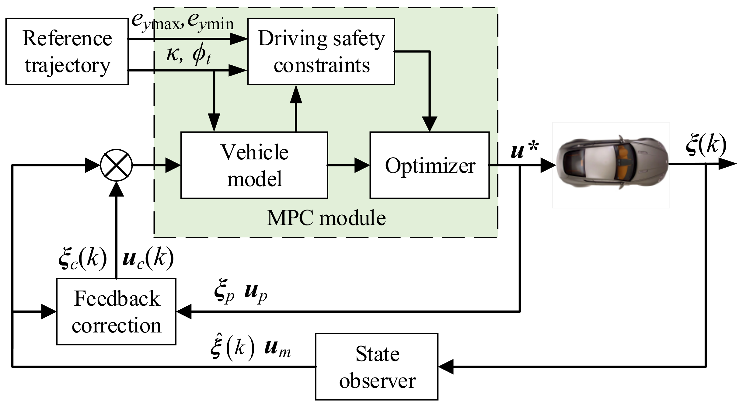
2.2. Framework Overview

The framework of the proposed MPC scheme is shown in Figure 2. The MPC module consists of three blocks: the vehicle model, driving safety constraints and optimizer. As the vehicle states cannot always be measured, a state observer is necessary for state estimation. At each step, the estimated state ${\widehat{\xi }}_k$ and the measured control action $u_m$ together with the $u_c$ and ${\xi }_c$ obtained from the feedback correction module are used to generate modified vehicle state ${\xi }_k={\widehat{\xi }}_k+k_1\ast {\xi }_c$ and modified control input $u_k=u_m+k_2\ast u_c$, where $k_1,k_2$ are integral coefficients. Accordingly, the vehicle model is developed while accounting for the road curvature $\kappa$ and bank angle ${\varphi }_t$. Then, safe driving constraints are designed to prevent sideslips, rollovers and exceeding road boundaries. Finally, an MPC problem is formulated and solved to generate the optimal control sequence $u^{\ast }$.

3. Vehicle Dynamics Modeling and Discretization

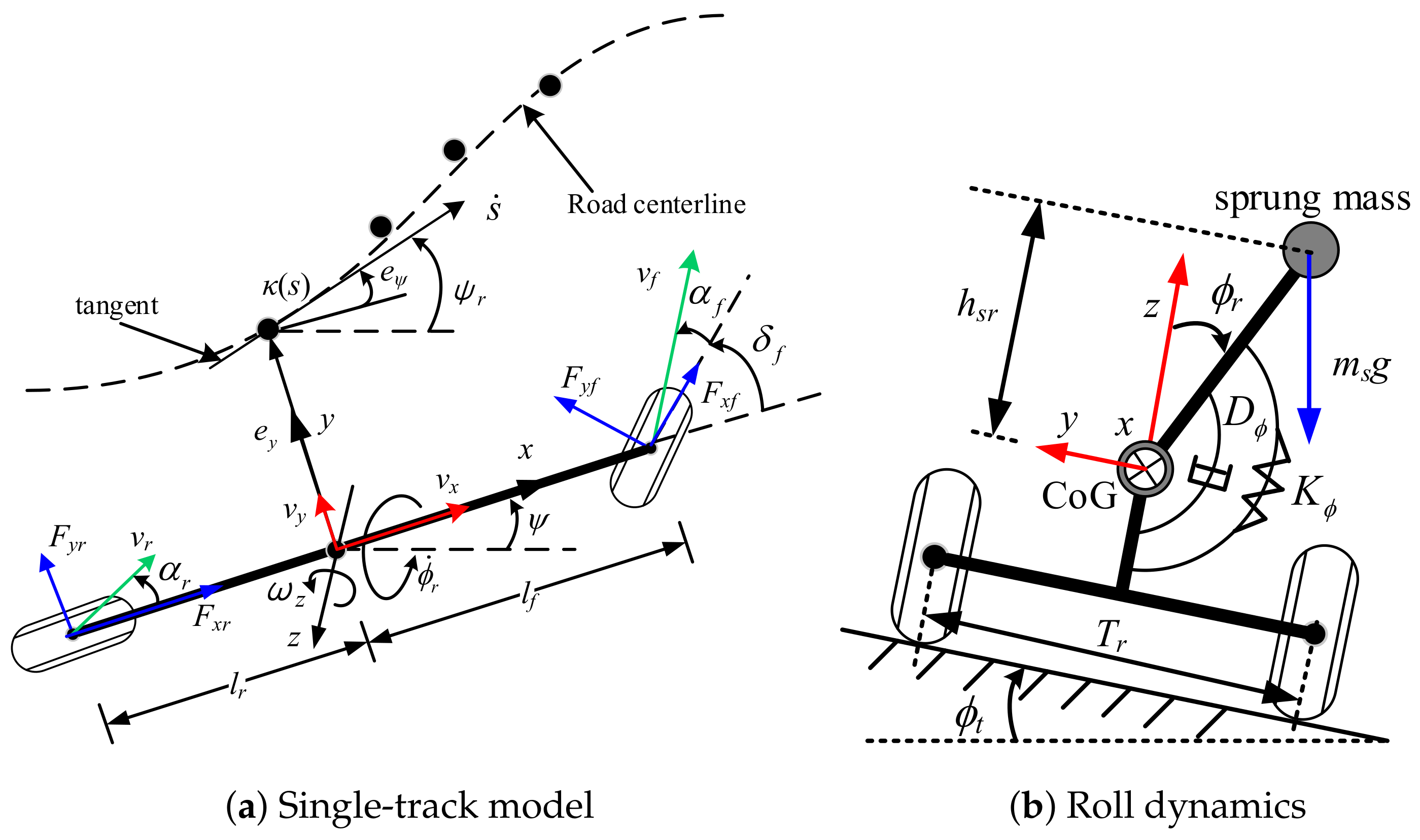
3.1. Dynamics Modeling

For a high-speed AGV, the vehicle generally steers with a large radius and small front steering angle. Therefore, the track width is neglectable with respect to its cornering radius. Thus, it is reasonable to use a spatial single-track vehicle model, as shown in Figure 3. The vehicle dynamics can be expressed as [21]:

$$m{\dot{v}}_x=a_x+m{v}_y{\omega }_z-m_s{h}_{sr}{\omega }_z{\omega }_x$$

(1a)

$$m{\dot{v}}_y=a_y-m{v}_x{\omega }_z-mgsin\left({\varphi }_t\right)+m_s{h}_{sr}{\dot{\omega }}_x$$

(1b)

$$I_z{\dot{\omega }}_z=\left(l_f{F}_{yf}-l_r{F}_{yr}\right)$$

(1c)

$${\dot{\varphi }}_r={\omega }_x$$

(1d)

$$I_x{\dot{\omega }}_x=m_s{h}_{sr}({\dot{v}}_y+v_x{\omega }_z)+m_{s}g{h}_{sr}sin\left(\varphi \right)-M_R$$

(1e)

where $a_x=(F_{xf}+F_{xr}-F_R)/m$, $F_{xf}$, $F_{xr}$ are the longitudinal forces at the front/rear tire, $F_R$ represents the dissipative forces, including aerodynamic drag force, rolling resistance friction force, etc., $a_y=(F_{yf}+F_{yr})/m$, $F_{yf}$, $F_{yr}$ are the lateral forces at the front/rear tire, $M_R=K_{\varphi }{\varphi }_r+D_{\varphi }{\omega }_x$, $K_{\varphi }$ and $D_{\varphi }$ are the suspension roll damping and stiffness, m is the total vehicle mass, $m_s$ is the sprung mass, $\psi$ and ${\omega }_z$ are the yaw angle and yaw rate, $h_{sr}$ is the height of the sprung mass from the roll center, $l_f$, $l_r$ are the distances from the CoG to the front and rear axle along the vehicle’s x-axis, g is the gravitational acceleration, $v_x$, $v_y$ are the longitudinal and lateral velocities of the CoG and ${\varphi }_r$, ${\omega }_x$ and ${\dot{\omega }}_x$ are the roll dynamics (angle, rate and acceleration) of the sprung mass, respectively. ${\varphi }_t$ is the road bank and assumes ${\dot{\varphi }}_t\approx 0$, ${\varphi }_r$ is the roll angle of the sprung mass to the vehicle’s z-axis. $\varphi ={\varphi }_t+{\varphi }_r$, $I_z$ is the moment of inertia about the vehicle’s z-axis. $I_x$ is the moment of inertia of the sprung mass with respect to the roll center. The cross products of the mass moment of inertia are neglected.

The relative motions of the AGV with respect to the road curvilinear coordinate system are:

$$\begin{array}{cc}\hfill {\dot{e}}_y=& v_{x}sin\left(e_{\psi }\right)+v_{y}cos\left(e_{\psi }\right)\approx v_x{e}_{\psi }+v_y\hfill \end{array}$$

(2)

$$\begin{array}{cc}\hfill {\dot{e}}_{\psi }=& {\omega }_z-\kappa v_x\hfill \end{array}$$

(3)

where, $e_y$ is the cross track error and $e_{\psi }$ is the difference between the vehicle heading angle, $\psi$, and the road centerline angle, ${\psi }_r$. $\kappa$ is the road centerline curvature.

Equations (1)–(3) are derived under the following assumptions:

• $e_{\psi }$, ${\delta }_f$ and $\varphi$ satisfy the small angle assumption;
• The vehicle pitch/actuators dynamics can be neglected, and the steering system is rigid;
• The disturbances such as wind lateral thrust are not considered.

In this work, we mainly focus on the lateral and roll dynamics of AGVs; thus, $a_x$ is assumed to be constant. Considering a front-wheel-driven vehicle, then $F_{xr}=0$. The longitudinal front tire force $F_{xf}$ can be computed as:

$$F_{xf}=m{a}_x+F_R$$

(4)

As the nonlinearity of lateral tire forces, $F_{yf}$ and $F_{yr}$, pose a significant challenge to real-time optimization, we use a linearized tire force model, as illustrated in Figure 4. Then, the lateral tire forces are approximated as [30]:

$$F_{y\ast }={\overline{C}}_{\alpha \ast }{\alpha }_{\ast }$$

(5)

where ${\overline{C}}_{\alpha \ast }$ is the equivalent cornering stiffness at ${\alpha }_{\ast }=0$. This linearization will lead to diverging from the actual tire forces at high sideslip angle; however, this problem can be avoided by enforcing a sideslip angle threshold, ${\alpha }_{lim}$.

The tire slip angles, ${\alpha }_f$ and ${\alpha }_r$, can be linearized using small angle approximations:

$${\alpha }_f=arctan(\frac{v_y+l_f{\omega }_z}{v_x})-{\delta }_f\approx \frac{v_y+l_f{\omega }_z}{v_x}-{\delta }_f$$

(6)

$${\alpha }_r=arctan(\frac{v_y-l_r{\omega }_z}{v_x})\approx \frac{v_y-l_r{\omega }_z}{v_x}$$

(7)

Let $\xi ={\left[v_y,{\omega }_z,{\omega }_x,{\varphi }_r,e_y,e_{\psi }\right]}^T$ denote the state vector, ${\mathit{u}}_1={\delta }_f$ denote the control input and ${\mathit{u}}_2={\left[{\varphi }_t,\kappa \right]}^T$ denote the auxiliary input, assumed known a priori. By combining (1)–(7), a linear time-varying vehicle model, concerning the lateral and roll dynamics, can be obtained as:

$$\dot{\xi }=\mathit{A}\xi +{\mathit{B}}_1{\mathit{u}}_1+{\mathit{B}}_2{\mathit{u}}_2$$

(8)

The matrix $\mathit{A}$, ${\mathit{B}}_1$ and ${\mathit{B}}_2$ used in (10) is:

$$\begin{array}{ccc}\hfill \mathit{A}& =\left[\begin{array}{cccccc}\frac{I_x{\mathsf{\Theta }}_1}{{\mathsf{\Theta }}_4}& \frac{I_x{\mathsf{\Theta }}_2}{{\mathsf{\Theta }}_4}-v_x& \frac{-{\mathsf{\Theta }}_6{D}_{\varphi }}{{\mathsf{\Theta }}_4}& \frac{{\mathsf{\Theta }}_6{\mathsf{\Theta }}_5}{{\mathsf{\Theta }}_4}& 0& 0\\ \frac{{\mathsf{\Theta }}_2}{I_z}& \frac{{\mathsf{\Theta }}_3}{I_z}& 0& 0& 0& 0\\ \frac{{\mathsf{\Theta }}_6{\mathsf{\Theta }}_1}{{\mathsf{\Theta }}_4}& \frac{{\mathsf{\Theta }}_6{\mathsf{\Theta }}_2}{{\mathsf{\Theta }}_4}& \frac{-m{D}_{\varphi }}{{\mathsf{\Theta }}_4}& \frac{m{\mathsf{\Theta }}_5}{{\mathsf{\Theta }}_4}& 0& 0\\ 0& 0& 1& 0& 0& 0\\ 1& 0& 0& 0& 0& v_x\\ 0& 1& 0& 0& 0& 0\end{array}\right],{\mathit{B}}_1\hfill & \hfill =\left[\begin{array}{c}\frac{-I_x{\overline{C}}_{\alpha f}}{{\mathsf{\Theta }}_4}\\ -\frac{l_f{\overline{C}}_{\alpha f}}{I_z}\\ -\frac{{\mathsf{\Theta }}_6{\overline{C}}_{\alpha f}}{{\mathsf{\Theta }}_4}\\ 0\\ 0\\ 0\end{array}\right],{\mathit{B}}_2=\left[\begin{array}{cc}-g& 0\\ 0& 0\\ 0& 0\\ 0& 0\\ 0& 0\\ 0& v_x\end{array}\right]\end{array}$$

with: ${\mathsf{\Theta }}_1=\left({\overline{C}}_{\alpha f}+{\overline{C}}_{\alpha r}\right)/\phantom{\left({\overline{C}}_{\alpha f}+{\overline{C}}_{\alpha r}\right)v_x}{v}_x$, ${\mathsf{\Theta }}_2=\left(l_f{\overline{C}}_{\alpha f}-l_r{\overline{C}}_{\alpha r}\right)/\phantom{\left(l_f{\overline{C}}_{\alpha f}-l_r{\overline{C}}_{\alpha r}\right)v_x}{v}_x$, ${\mathsf{\Theta }}_3=\left(l_f^2{\overline{C}}_{\alpha f}+l_r^2{\overline{C}}_{\alpha r}\right)/\phantom{\left(l_f^2{\overline{C}}_{\alpha f}+l_r^2{\overline{C}}_{\alpha r}\right)v_x}{v}_x$, ${\mathsf{\Theta }}_4=\left(I_{x}m-m_s^2{h}_{sr}^2\right)$, ${\mathsf{\Theta }}_5=\left(m_s{h}_{sr}g-K_{\varphi }\right)$, ${\mathsf{\Theta }}_6=m_s{h}_{sr}$

3.2. Model Discretization

The obstacle avoidance objective of the high-speed AGV controller necessitates a long enough prediction horizon to safely anticipate upcoming obstacles. However, if the controller execution time step is used as the prediction time step throughout the full horizon, the total number of time steps required is prohibitively large for real-time implementation. Alternatively, selecting a large time step for the full horizon degrades the controller’s performance in predicting near-term vehicle behavior, which is necessary when reacting to unexpected challenges of vehicle stabilization.

To address this issue, the prediction horizon used in this work is split into two portions at time step $N_s$. The initial portion is comprised of small time steps of size $t_s$, which is equal to the execution time step of the controller, to accurately capture near-term vehicle behavior. The latter portion is comprised of larger time steps of size $t_l$ to extend the horizon to incorporate upcoming obstacles in the long-term. These variable time steps provide a good balance between the prediction accuracy and the computational burden. Besides, $t_l$, $N_s$ and $N_p$ are chosen according to experimental experience.

By virtue of matrix exponentials, the vehicle dynamics model (8) is discretized using zero-order hold (ZOH) and first-order hold (FOH) methods on the initial portion and latter portion of the prediction horizon, respectively. The discretized vehicle model can be expressed as:

$${\xi }^{\left(k+1\right)}={\mathit{A}}_s{\xi }^{\left(k\right)}+{\mathit{B}}_{s1}{u}_1^{\left(k\right)}+{\mathit{B}}_{s2}{u}_2^{\left(k\right)},\forall k=1,\cdots ,N_s$$

(9)

$${\xi }^{\left(k+1\right)}={\mathit{A}}_l{\xi }^{\left(k\right)}+{\mathit{B}}_{l1}{u}_{aug}^{\left(k\right)}+\mathit{B}{u}_{aug}^{\left(k+1\right)}\forall k=N_s+1,\cdots ,N_p-1$$

(10)

where ${\mathit{A}}_s={\mathit{I}}_6+\mathit{A}\times t_s$, ${\mathit{B}}_{s1}={\mathit{B}}_1\times t_s$, ${\mathit{B}}_{s2}={\mathit{B}}_2\times t_s$ and ${\mathit{A}}_l={\mathit{I}}_6+\mathit{A}\times t_l+{(\mathit{A}\times t_l)}^2/2$, ${\mathit{B}}_{l1}={\mathsf{\Gamma }}_1-{\mathsf{\Gamma }}_2$, ${\mathit{B}}_{l2}={\mathsf{\Gamma }}_2$, ${\mathsf{\Gamma }}_1=[B_1,B_2]\times t_l+\mathit{A}\times [B_1,B_2]\times t_l^2/2$, ${\mathsf{\Gamma }}_2=[B_1,B_2]\times t_l/2$, $u_{aug}={[u_1,u_2]}^T$.

4. MPC Scheme Design

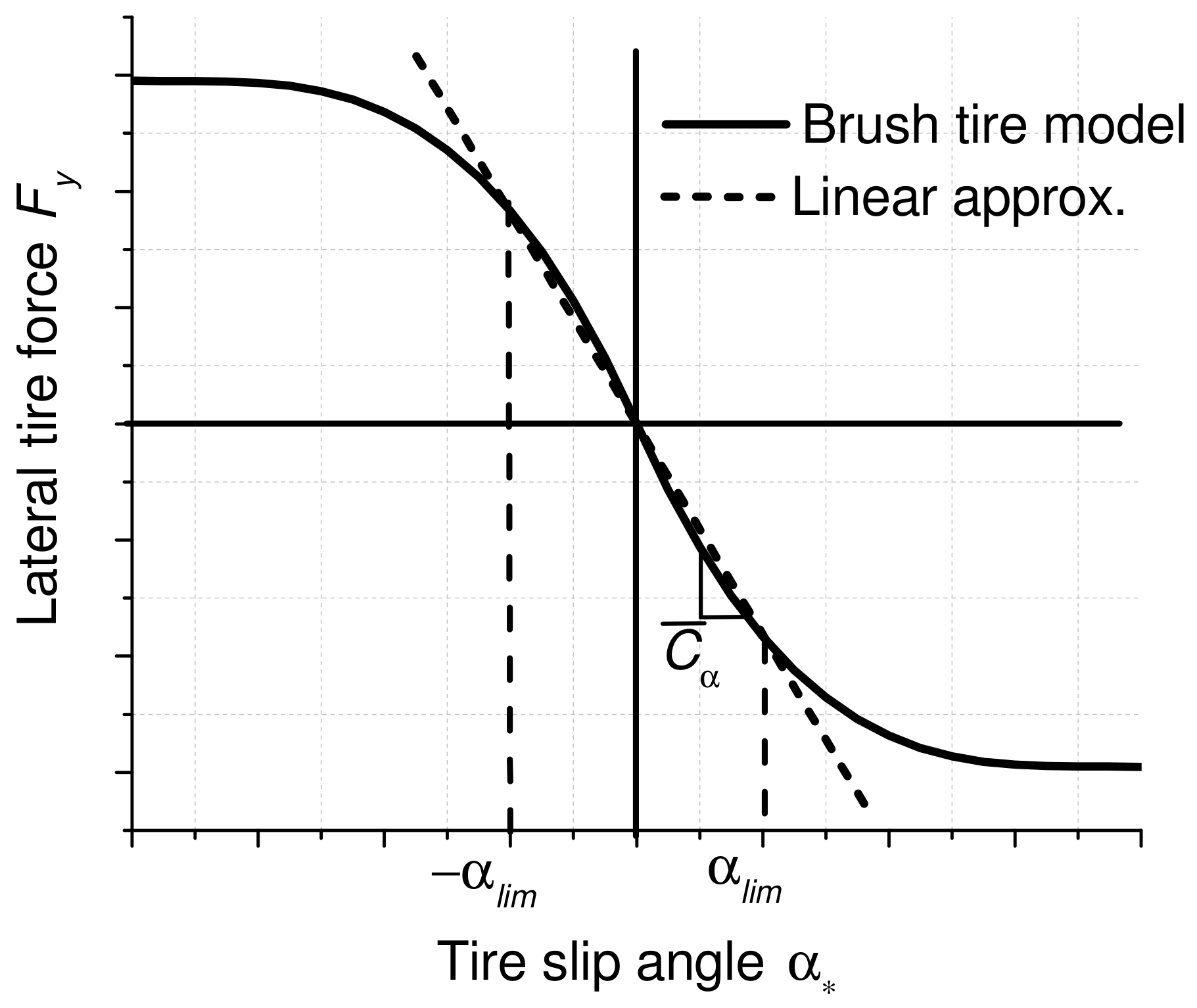
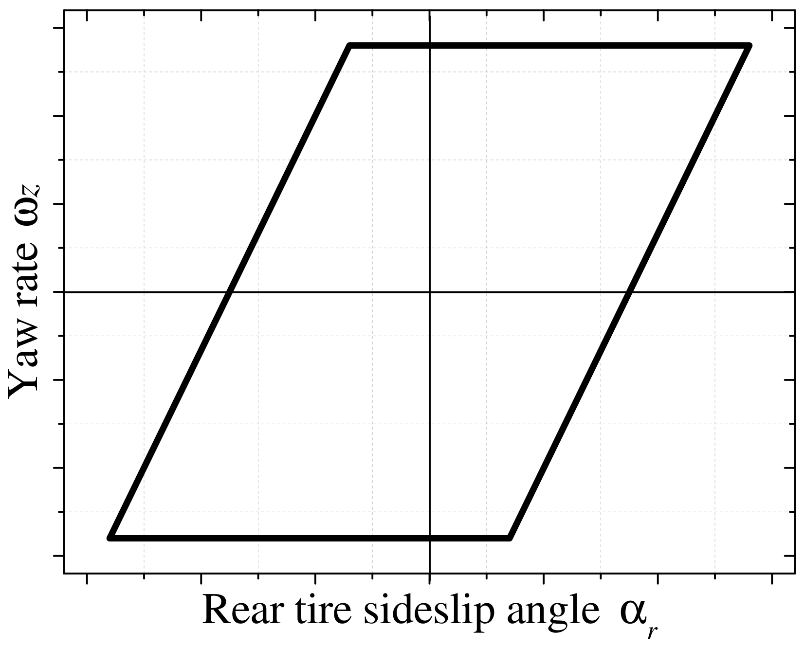
4.1. Sideslip Constraints

Generally, the sideslip first starts on the rear tire; thus, the sideslip constraint is enforced as bounds on the vehicle’s rear tire sideslip angle (${\alpha }_r$) and yaw rate (${\omega }_z$). The range of ${\alpha }_r$ is defined from the linear tire model used in (7) and converted into a bound on vehicle states with (5):

$$\left|\left(v_y-l_r{\omega }_z\right)/\phantom{\left(v_y-l_{r}r\right)v_x}{v}_x\right|\le {\alpha }_{r,lim}$$

(11)

To determine an appropriate bound on yaw rate (${\omega }_z$), a steady-state analysis is used based on (1b). This ensures that the vehicle does not exceed the linear region of the brush tire model and yields a maximum sustained yaw rate as:

$$\left|{\omega }_z+\frac{g}{v_x}{\varphi }_t\right|\le \frac{{\overline{C}}_{\alpha r}{\alpha }_{r,lim}\left(1+l_r/\phantom{l_r{l}_f}{l}_f\right)}{m{v}_x}$$

(12)

Assuming real-time estimation of ${\overline{C}}_{\alpha r}$ is available, the vehicle envelope described is easily calculated in real time. Let ${\mathit{S}}_{sh}^{\left(k\right)}={\left[{\alpha }_{r,slack},{\omega }_{z,slack}\right]}^T$ represent the slacks to the sideslip constraint, then (11) and (12) can be compactly represented as the following linear inequality for each time step k into the prediction horizon:

$$-{\mathit{G}}_{\mathrm{sh}}-{\mathit{S}}_{\mathrm{sh}}^{\left(k\right)}\le {\mathit{H}}_{\mathrm{sh}}{\xi }^{\left(k\right)}+{\mathit{P}}_{\mathrm{sh}}{u}_2^{\left(k\right)}\le {\mathit{G}}_{\mathrm{sh}}+{\mathit{S}}_{\mathrm{sh}}^{\left(k\right)}$$

(13)

with:

$$\begin{array}{c}\hfill {\mathit{H}}_{\mathrm{sh}}=\left[\begin{array}{cccccc}1/\phantom{1v_x}{v}_x& -l_r/\phantom{l_r{v}_x}{v}_x& 0& 0& 0& 0\\ 0& 1& 0& 0& 0& 0\end{array}\right],{\mathit{P}}_{\mathrm{sh}}=\left[\begin{array}{cc}0& 0\\ g/\phantom{g{v}_x}{v}_x& 0\end{array}\right],{\mathit{G}}_{\mathrm{sh}}=\left[\begin{array}{c}{\alpha }_{r,lim}\\ {\overline{C}}_{\alpha r}{\alpha }_{r,lim}\left(1+l_r/\phantom{l_r{l}_f}{l}_f\right)/\phantom{{\overline{C}}_{\alpha r}{\alpha }_{r,lim}\left(1+l_r/\phantom{l_r{l}_f}{l}_f\right)m{v}_x}m{v}_x\end{array}\right]\end{array}$$

where ${\xi }^{(k)}$ indicates the vehicle state at the k-th time step into the prediction horizon.

The bounds (11) and (12) define a linear time-varying closed envelope, as shown in Figure 5. (11) serves as the basis for upper and lower bounds, and (12) defines the left and right bounds. Vehicle stability is guaranteed for all states in this envelope. That is, at any point within this envelope, a steering command exists such that the vehicle can safely remain inside. However, exceeding these bounds does not necessarily result in instability, but for states outside the envelope, there is no guarantee that a control input exists to move the system closer to the boundary in the next time step. Regions of the state space beyond the sideslip bounds entail nonlinearity of the rear tire force, which can be difficult to control. Regions directly past the yaw rate bounds, however, do not entail tire saturation and can lead back to the handling envelope without a spin. Often, vehicle states first exceed the yaw rate bound on the way to exceeding the side slip bound, which motivates using the yaw rate bound. However, small violations of the yaw rate bound by itself can occur without ensuing sideslip violations, and this behavior is considered acceptable in motion control.

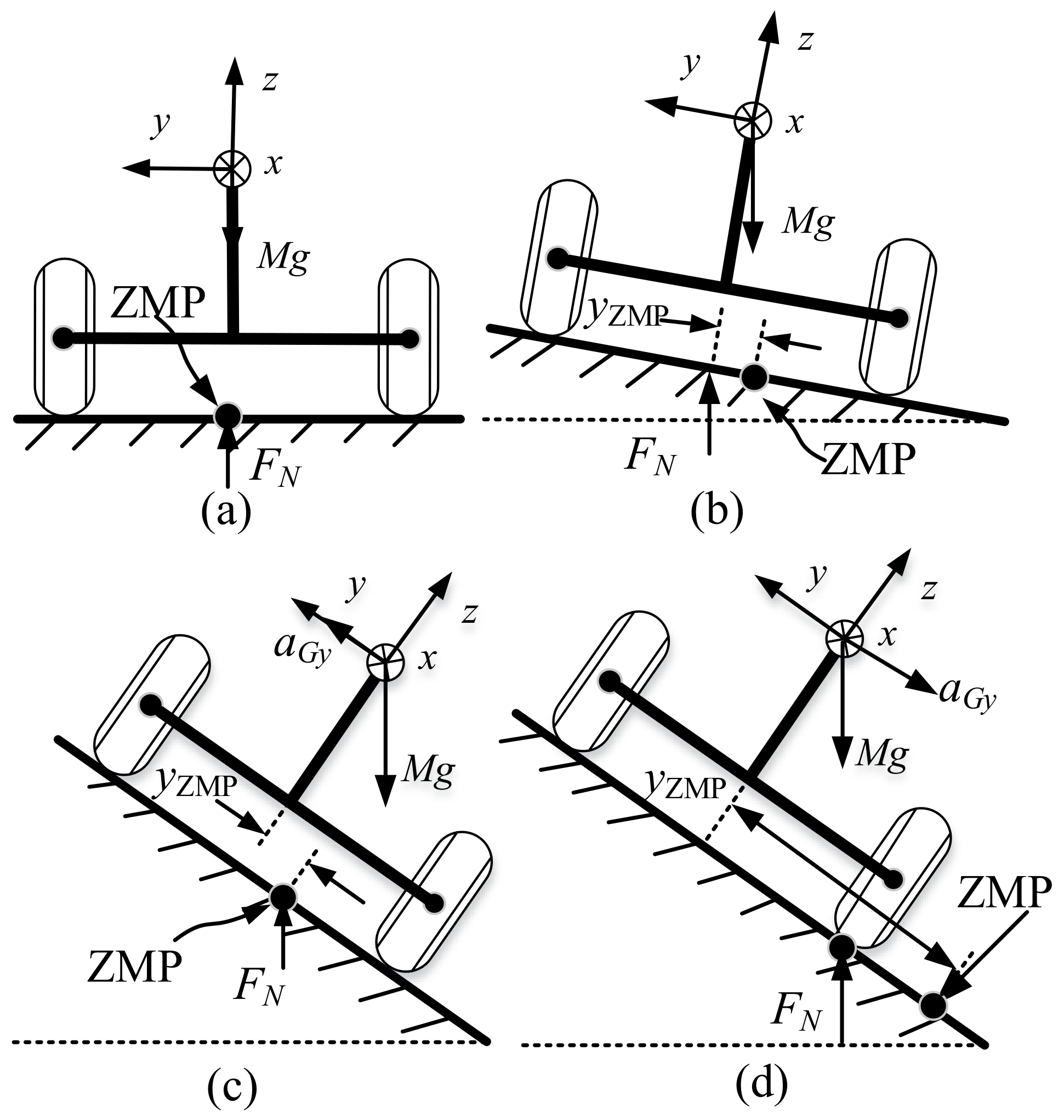
4.2. Rollover Constraints

A key challenge in preventing the rollover of the AGV is the prediction of rollover onset, especially in the presence of the road bank and the median slope. This work utilizes ZMP as a direct measure of a vehicle rollover threat index. The ZMP is defined as the point on the ground where the summation of tipping moments, due to gravity and inertia forces, equals zero, as illustrated in Figure 6.

When the AGV is driving on a horizontal road, the reaction force $F_N$ acting directly beneath the AGV’s center of mass, this reaction point is the ZMP, as shown in Figure 6a. When driving on a road with a bank angle, as shown in Figure 6b, the reaction force $F_N$ shifts in order to balance the vehicle’s weight and satisfy the definition of ZMP. The lateral acceleration caused by turning will also shift the reaction force as shown in Figure 6c. Eventually, there exists an angle or lateral acceleration, as in Figure 6d, where the reaction force is no longer able to balance the vehicle’s weight (or inertial dynamics) and the ZMP moves outside the support polygon, leading to the rollover of the AGV.

Although the location of ZMP exists in three-dimensional space, only its coordinate along the vehicle’s body-fixed y-axis, termed as $y_{ZMP}$, is of interest for vehicle rollover prevention. The regularized $y_{ZMP}$ with respect to half of the track width ($T_r/\phantom{T_{r}2}2$) is written as:

$${\overline{y}}_{ZMP}=\frac{2}{T_r}\left(h_{sr}\varphi +\frac{h_{sr}}{g}\left({\dot{v}}_y+{\omega }_z{v}_x\right)-\frac{I_x}{mg}{\dot{\omega }}_x\right)$$

(14)

(14) can be rearranged as:

$${\overline{y}}_{ZMP}={\mathit{N}}_1{\dot{\xi }}^{\left(k\right)}+{\mathit{N}}_2{\xi }^{\left(k\right)}+{\mathit{N}}_3{\mathit{u}}_2$$

(15)

with:

$${\mathit{N}}_1=\left[\begin{array}{cccccc}2h_{sr}/\phantom{2h\left(g{T}_r\right)}\left(g{T}_r\right)& 0& -2I_x/\phantom{2I_x\left(mg{T}_r\right)}\left(mg{T}_r\right)& 0& 0& 0\end{array}\right],{\mathit{N}}_2=\left[\begin{array}{cccccc}0& 2h_{sr}{v}_x/\phantom{2h{v}_{x}g{T}_r}g{T}_r& 0& 2h_{sr}/\phantom{2h{T}_r}{T}_r& 0& 0\end{array}\right],$$

and ${\mathit{N}}_3=\left[\begin{array}{cc}2h_{sr}/\phantom{2h_{sr}{T}_r}{T}_r& 0\end{array}\right]$.

Then, the constraint for rollover prevention is:

$$-{\overline{y}}_{ZMP,max}\le {\overline{y}}_{ZMP}\le {\overline{y}}_{ZMP,max}$$

(16)

where ${\overline{y}}_{ZMP,max}$ is the threshold of ZMP.

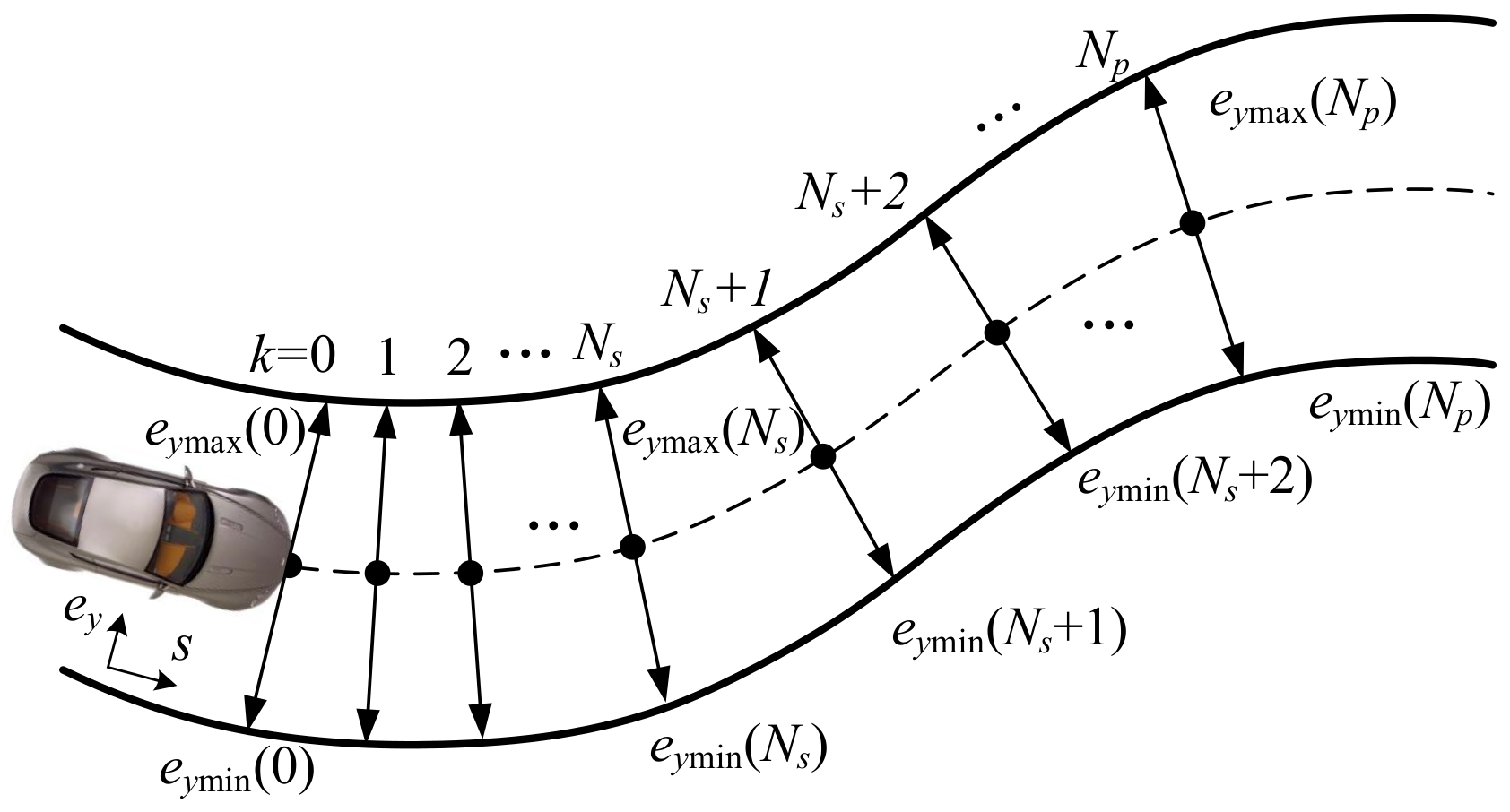
4.3. Lateral Safety Corridor

To ensure driving safety, the AGV needs to be fully contained within the feasible region, determined by the environmental constraints such as road boundaries or lane marks. Here, we define a lateral safety corridor, according to the pre-defined longitudinal position and correlated with the road properties, to represent the feasible region. The lateral safety corridor is expressed as time-varying upper and lower bounds on the AGV’s cross track error $(e_y)$.

Figure 7 illustrates the methodology to generate the lateral safety corridor. Based on the constant longitudinal acceleration assumption, the reference road can be sampled at discrete points along the road centerline, which correspond to the AGV’s future position k steps into the prediction horizon. The feasible lateral gap at each time step k is identified mainly considering the lane boundaries’ and vehicles’ effective width. Starting at the AGV’s current position, the lateral safety corridor is generated by linking the adjacent feasible gaps throughout the prediction horizon. Therefore, the lateral safety corridor is defined as a set of lateral deviation bounds $e_{ymax}$ and $e_{ymin}$ and can be compactly written as:

$${\mathit{H}}_{\mathrm{env}}{\xi }^{\left(k\right)}\le {\mathit{G}}_{\mathrm{env}}^{\left(k\right)}$$

(17)

with:

$${\mathit{H}}_{\mathrm{env}}=\left[\begin{array}{cccccc}0& 0& 0& 0& 1& 0\\ 0& 0& 0& 0& -1& 0\end{array}\right],{\mathit{G}}_{\mathrm{env}}^{\left(k\right)}=\left[\begin{array}{c}{e}_{y,max}^k-d_s\\ -e_{y,min}^k+d_s\end{array}\right]$$

This provides a convex method of enforcing environmental constraints on the position of AGVs. $d_s$ is a user-defined comfort distance.

Moreover, the steering input should also satisfy the limits of the actuator system:

$$\left|{\delta }_f\right|\le {\delta }_{f,max}$$

(18)

$$\left|\Delta {\delta }_f\right|\le \Delta {\delta }_{f,max}$$

(19)

where ${\delta }_{f,max}$ and $\Delta {\delta }_{f,max}$ reflect the maximum allowable steering angle and the physical slew rate capabilities of the vehicle steering system.

4.4. MPC Problem Formulation

The primary task of the stabilization control of high-speed AGVs is to ensure safe vehicle operation within the previously-defined constraints. This is realized by expressing the stabilization control as an optimal control problem to be evaluated over a finite prediction horizon, formulated as:

$$\underset{\xi ,{\delta }_f,k=0,\cdots ,N_p}{minimize}J=\sum _k\left(W_{e\psi }{\left(e_{\psi }^{\left(k\right)}\right)}^2+W_{ey}{\left(e_y^{\left(k\right)}\right)}^2\right)$$

(20a)

$$+\sum _k{W}_{\delta f}{\left({\delta }_f^{\left(k\right)}-{\delta }_f^{\left(k-1\right)}\right)}^2$$

(20b)

$$+\sum _k{W}_{\mathrm{sh}}^T{S}_{sh}^{\left(k\right)}{W}_{\mathrm{sh}}$$

(20c)

$$\mathrm{s}.\mathrm{t}.{\xi }^{\left(k+1\right)}={\mathit{A}}_s{\xi }^{\left(k\right)}+{\mathit{B}}_{s1}{\mathit{u}}_1^{\left(k\right)}+{\mathit{B}}_{s2}{\mathit{u}}_2^{\left(k\right)}$$

(20d)

$${\xi }^{\left(k+1\right)}={\mathit{A}}_l{\xi }^{\left(k\right)}+{\mathit{B}}_{l1}{{\mathit{u}}_{aug}}^{\left(k\right)}+{\mathit{B}}_{l2}{{\mathit{u}}_{aug}}^{\left(k+1\right)}$$

(20e)

$$\left|{\mathit{H}}_{sh}^k{\xi }^{\left(k\right)}+{\mathit{P}}_{sh}{\mathit{u}}_2^{\left(k\right)}\right|\le {\mathit{G}}_{sh}^k+{\mathit{S}}_{sh}^{\left(k\right)}$$

(20f)

$$\left|{\overline{y}}_{ZMP}\right|\le {\overline{y}}_{ZMP,max}$$

(20g)

$${\mathit{H}}_{\mathrm{env}}{\xi }^{\left(k\right)}\le {\mathit{G}}_{\mathrm{env}}^{\left(k\right)}$$

(20h)

$$\left|{\delta }_f\right|\le {\delta }_{f,max}$$

(20i)

$$\left|\Delta {\delta }_f\right|\le \Delta {\delta }_{f,max}$$

(20j)

In this formulation, the variables to be optimized are the front wheel steering angle (${\delta }_f$) and the slack variables on the constraints $S_{sh}$. The tunable parameters are $W{\delta }_f$, $W{e}_y$, $W{e}_{\psi }$ and the slack variable costs factor $W_{sh}$. The cost function consists of three terms: (20a) enforces penalty on the vehicle states deviation; (20b) establishes the trade-off between fast convergence and a smooth input trajectory; (20c) enforces the penalty for slack variables’ violations.

(20d) and (20e) are the discretized vehicle dynamics models, derived from (9) and (10). Constraints (20f), (20g) and (20h) enforce constraints on the sideslip envelope, ZMP and road boundaries, respectively. (20i) and (20j) enforce the physical limits of the steering system. With the choice of sufficiently large weighting coefficient $W_{sh}$, the cost term (20c) encourages zero-valued slack variables, resulting in optimal vehicle trajectories that adhere to the sideslip envelopes whenever possible.

Along with the relative value of $W{\delta }_f$, $W{e}_y$, $W{e}_{\psi }$ and $W_{sh}$, a hierarchy can be established between the collision, stabilization and smooth steering. Setting $(W{e}_y,W{e}_{\psi })\gg W_{sh}\gg W{\delta }_f$ encodes a prioritization of collision avoidance over vehicle stability and then over smooth steering. This prioritization allows the controller to selectively violate stability criteria if necessary to avoid a collision.

The optimization (20) resolves at each step; as is standard with MPC, only the optimal input for the first step into the prediction horizon, ${\delta }_f^{(0)}$, is executed. The convexity of the optimization problem allows for efficient real-time implementation. CVXGEN [31] generates a solver that is implemented on a Thinkpad W541 stationary computer with a quad-core i7-processor. The resulting controller is capable of solving the optimization problem in less than 50 ms, allowing for an execution rate of 20 Hz.

5. Simulations and Discussions

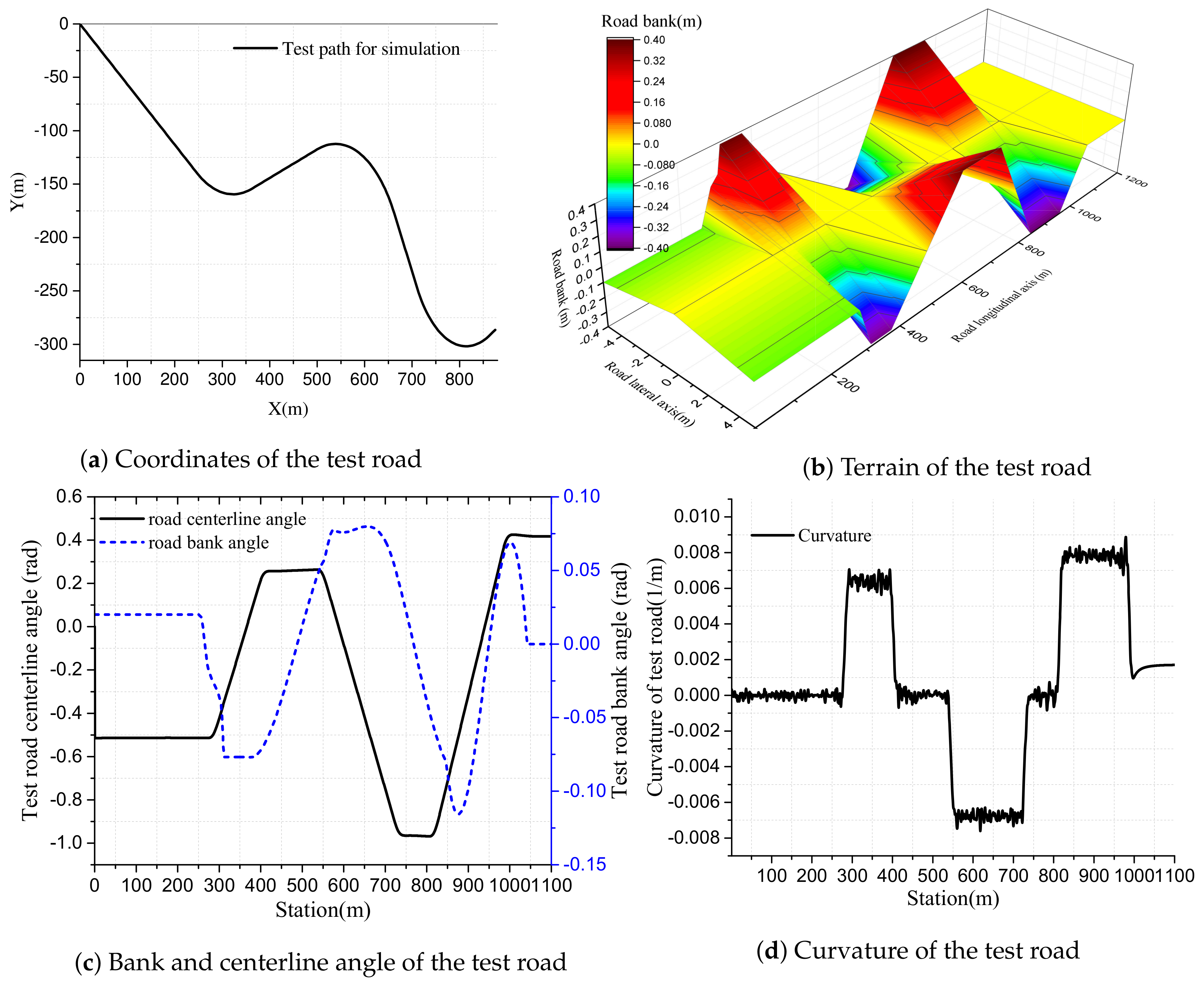
5.1. Simulation Settings

Simulations were carried out in the MATLAB/CarSim environment. A front-wheel drive D class SUV was used as the target AGV. The vehicle parameters and controller weights used in the proposed control scheme are shown in

Table 1. The parameter of the vehicle and weights of the MPC controller.

Parameters	Values (Unit)	Parameters	Values (Unit)	Parameters	Values (Unit)
m	1600 (kg)	${\overline{C}}_{\alpha f}$	−110,000 (N/rad)	$t_s$	0.05 (s)
$m_s$	1430 (kg)	${\overline{C}}_{\alpha r}$	−92,000 (N/rad)	$t_l$	0.5 (s)
$I_x$	700. 7 (kg· m2)	$K_{\varphi }$	145,330 (N· m/rad)	$N_s$	10
$I_z$	2059.2 (kg· m2)	$D_{\varphi }$	4500 (N· m· s/rad)	$N_p$	20
$l_f$	1.12 (m)	g	9.81 (m/s2)	$W_{ey},W_{e\psi }$	500
$l_r$	1.48 (m)	${\delta }_{f,max}$	0.4 (rad)	$W_{sh}$	50
$T_r$	1.565 (m)	$\Delta {\delta }_{f,max}$	0.08 (rad/s)	$W_{\delta f}$	5
$h_{sr}$	0.68 (m)	${\alpha }_{r,lim}$	0.1 (rad)	$k_1$	0.5
$d_s$	0.5 (m)	${\overline{y}}_{ZMP,max}$	0.7	$k_2$	0.6

.

As shown in Figure 8, a testing road with three large continuous corners is employed. The coordinates and terrain of the test road are illustrated in Figure 8a,b. Figure 8c illustrates the centerline angle and bank angle of the test road. The curvature of the test road is shown in Figure 8d.

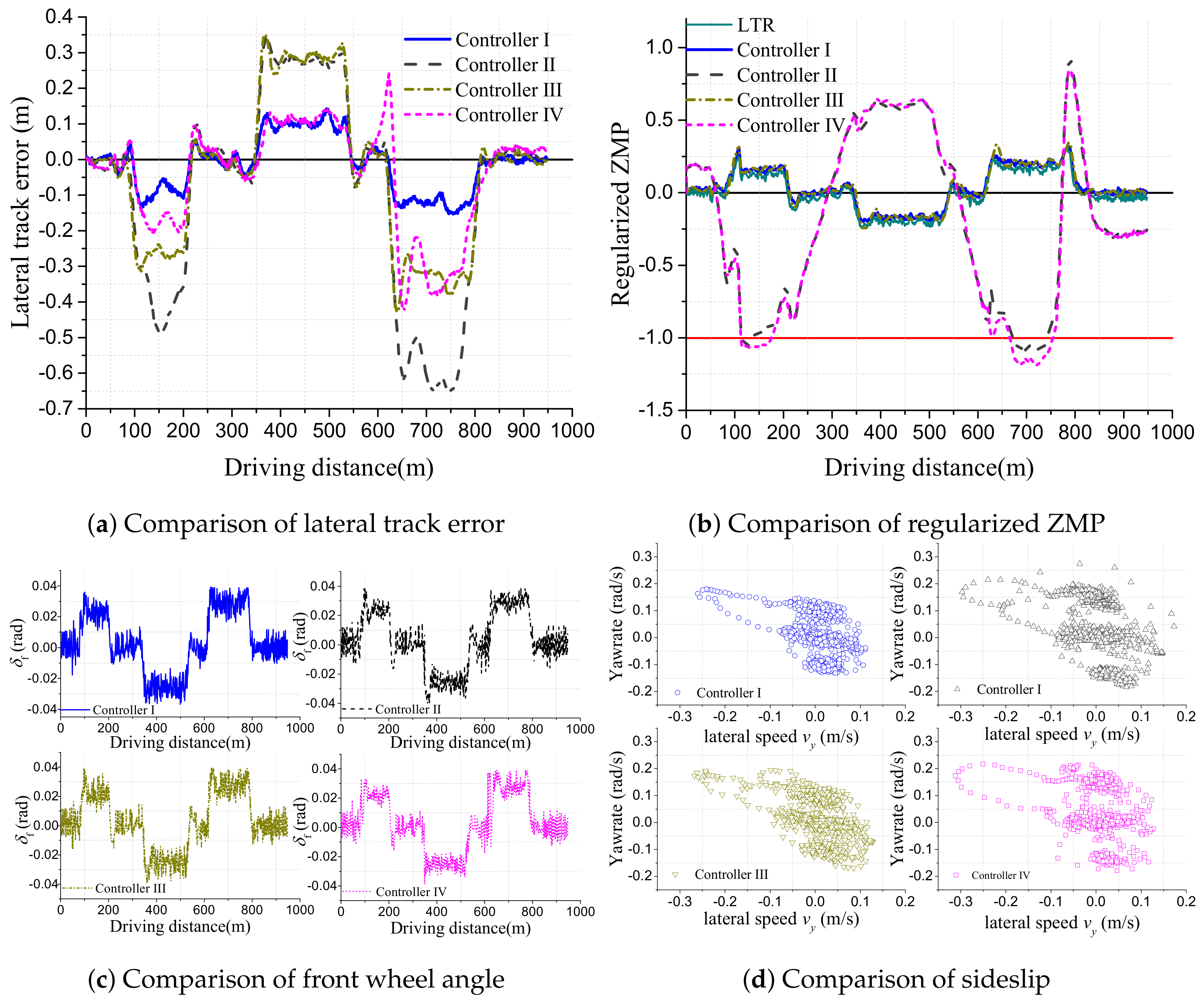
5.2. Performance Evaluation Considering Road Topography

To analyze the effect of considering road topography, four comparative MPC controllers are utilized for trajectory tracking of the test road, as shown in Figure 8. The desired velocity of AGV is set to be a constant of 72 km/h. Since the first 200 m of the test road is just a segment of a straight lane, we initialized the location of the AGV as 200 m behind the starting point of the test road.

• The MPC controller considers both road curvature and bank angle, as proposed in this work, denoted as Controller I;
• The MPC controller without consideration of road topography, i.e., setting ${\mathit{u}}_2={[0,0]}^T$, denoted as Controller II;
• The MPC controller only considers the effect of road bank angle, i.e., setting the second term of ${\mathit{u}}_2$ as zero, denoted as Controller III;
• The MPC controller only considers the effect of road curvature, i.e., setting the first term of ${\mathit{u}}_2$ as, denoted as Controller IV.

The comparison of the simulation results is shown in Figure 9. It can be seen from Figure 9a that the lateral track errors when considering the road curvature (Controller I and Controller IV) are significantly smaller than those not considering the road curvature (Controller II and Controller III). Thus, we can conclude that the road curvature has more influence on the lateral track error than that of road bank angle. As shown in Figure 9b, the regularized ZMPs when considering road bank angle (Controller I and Controller III) coincide nicely with the LTR. On the other hand, the regularized ZMPs when not considering road bank angle (Controller II and Controller IV) diverge significantly from the LTR. Thus, the road bank angle is validated to be an important factor for rollover prevention. Figure 9c illustrates the comparison of front wheel angle $({\delta }_f)$ during the simulations. We can see that the maximum of front wheel angle is less than 0.04 (rad), satisfying the actuator saturation limits. Figure 9d shows the comparison of sideslips in the plane of lateral velocity $v_y$ and yaw rate ${\omega }_z$. It can be seen that the traces of Controller I, considering both road curvature and bank angle, are more compact than those of the other three controllers. This validates that the proposed MPC scheme considering the effect of road topography can be used to ensure stabilization of high-speed AGVs.

Note that Controller I, considering the effects of both road curvature and bank angle, can provide better trajectory tracking performance than the other three controllers by limiting the lateral track error and the ${\overline{y}}_{ZMP}$ within 0.15 m and 0.3 m, respectively. Thus, it validates the necessity of considering road topography in the stabilization of high-speed AGVs.

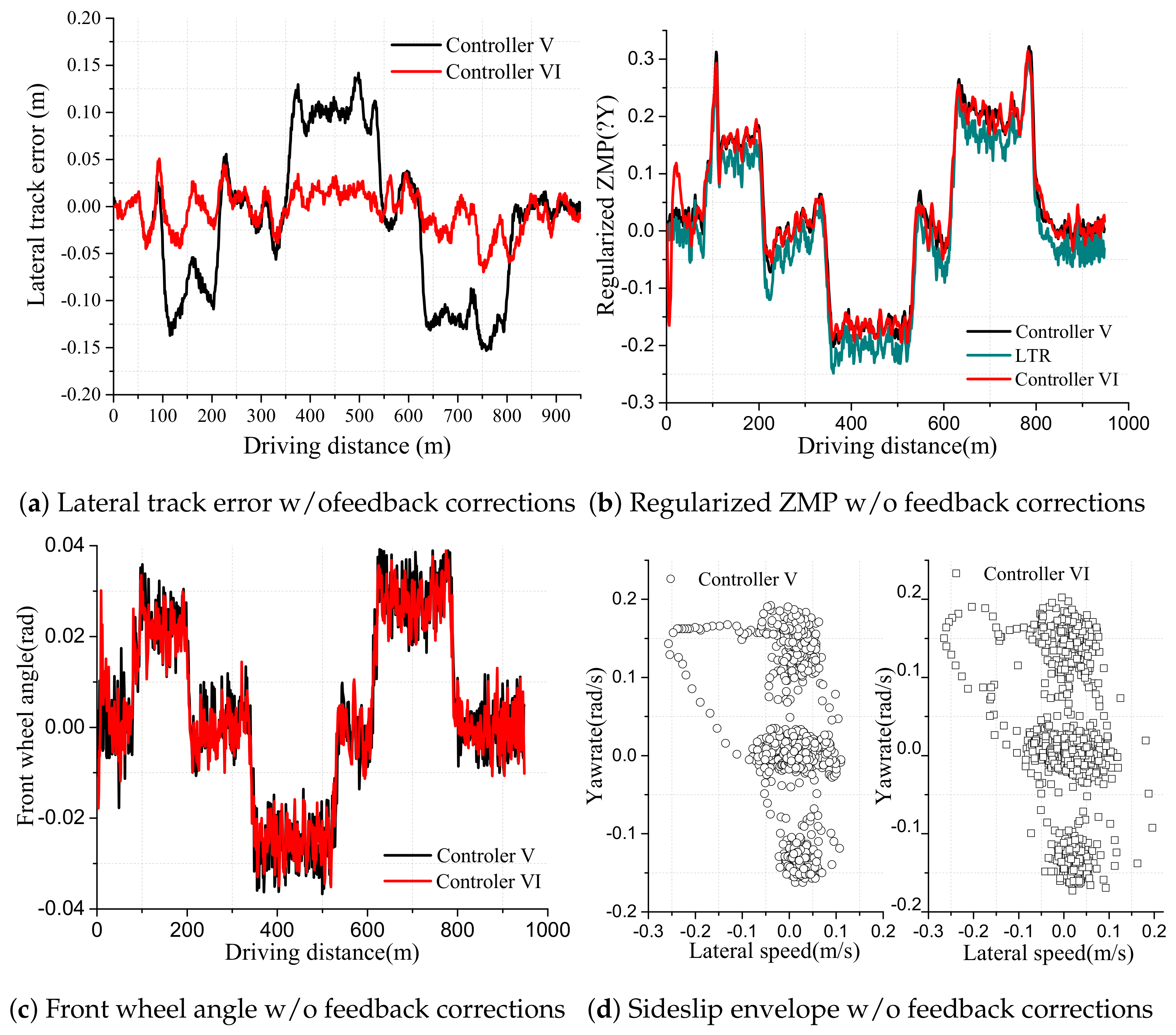
5.3. Performance Evaluation Considering Feedback Corrections

To analyze the effect of feedback corrections, the following two MPC controllers are utilized for the trajectory tracking of the test road, as shown in Figure 8.

• MPC controller without feedback corrections, setting $k_1=0,k_2=0$, denoted as Controller V;
• MPC controller with feedback corrections, as proposed in this work, denoted as Controller VI.

The simulated results are shown in Figure 10. The lateral track errors with/without feedback corrections are shown in Figure 10a. It can be seen that although both controllers can limit the lateral track error within 0.15 m, the tracking performance of Controller VI is obviously better than that of Controller V. The comparative simulation results on regularized ZMP, front wheel angle and sideslip envelope are shown in Figure 10b–d, respectively. It can be seen that the regularized ZMPs of both controllers coincide nicely with the LTR. The optimal front wheel angle inputs generated by both MPC controllers satisfy the actuator saturation limits. Both controllers are able to prevent excessive sideslips during trajectory tracking.

It can also be seen from Figure 10a that the lateral tracking error of Controller VI is very similar to that of Controller V in the straight lane section, and the main deviations appear in the curve section. These differences are most probably caused by the model mismatch in the curve sections, as the small angle assumption for (1)–(3) may lose validity. Moreover, the equivalent tire cornering stiffness coefficient ${\overline{C}}_{\alpha \ast }$ may differ from that at ${\alpha }_{\ast }=0$, leading to parameter uncertainties. The integration of the feedback corrections module in the MPC controller is able to mitigate the tracking errors caused by these model mismatches and parameter uncertainties, leading to better performance of Controller VI. Thus, we can conclude that using feedback corrections can compensate, to some extent, the unmodeled dynamics and parameter uncertainties.

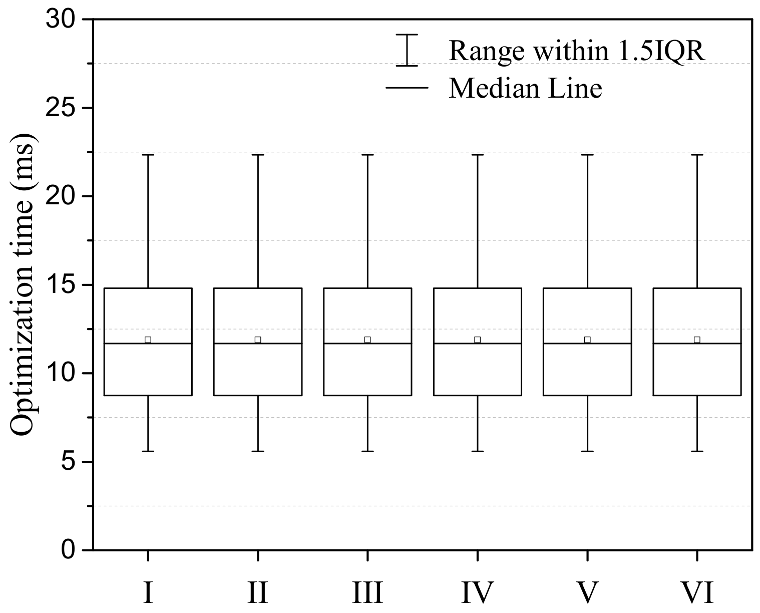
5.4. Real-Time Ability

The mean and standard deviation of the optimization time of the previously mentioned six controllers are shown in Figure 11. It can be seen that the mean of optimization time falls in the range of $[5,25]$ ms. Besides, the standard deviation of the optimization time is 0.0124 ms, indicating that the optimization time is relatively constant. Therefore, the proposed MPC scheme can be used in real-time applications.

6. Conclusions

This paper focuses on the stabilization control of high-speed autonomous ground vehicles considering the effect of road topography. The innovative aspects of the manuscript are:

• A vehicle model with roll dynamics is developed to account for the road curvature and bank angle. Variable time steps are utilized for model discretization, leading to long enough prediction for obstacle avoidance without compromising the prediction accuracy;
• The handling stability constraints, expressed as sideslip envelope and zero-moment-point, can be used to prevent excessive sideslip and rollover;
• An MPC control scheme is designed to generate the optimal steering sequence while satisfying the handling stability constraints. Comparative simulation results validate the effectiveness and real-time ability of the proposed control scheme.

Future work will consider the stabilization control of high-speed AGVs with time-varying accelerations. Real-vehicle experiments will also be carried out to verify the proposed control scheme.

References

1. Ozguner, U.; Acarman, T.; Redmill, K. Autonomous Ground Vehicles (Its); Artech House: Norwood, MA, USA, 2011; p. 277. [Google Scholar]
2. Jiang, Y.; Gong, J.W.; Xiong, G.M.; Chen, H.Y. Research on differential constraints-based planning algorithm for autonomous-driving vehicles. Zidonghua Xuebao/Acta Autom. Sin. 2013, 39, 2012–2020. [Google Scholar] [CrossRef]
3. Yan, J.; Qi, W.; Jianwei, G.; Huiyan, C. Research on Temporal Consistency and Robustness in Local Planning of Intelligent Vehicles. Acta Autom. Sin. 2015, 41, 518–527. [Google Scholar]
4. Gong, J.; Jiang, Y.; Xu, W. Model Predictive Control for Self-Driving Vehicles; Beijing Institute of Technology Press: Beijing, China, 2014. [Google Scholar]
5. Liu, K.; Gong, J.; Kurt, A.; Chen, H.; Ozguner, U. A model predictive-based approach for longitudinal control in autonomous driving with lateral interruptions. In Proceedings of the IEEE Intelligent Vehicles Symposium (IV), Los Angeles, CA, USA, 11–14 June 2017; pp. 359–364. [Google Scholar] [CrossRef]
6. Falcone, P.; Borrelli, F.; Asgari, J.; Tseng, H.E.; Hrovat, D. Predictive Active Steering Control for Autonomous Vehicle Systems. IEEE Trans. Control Syst. Technol. 2007, 15, 566–580. [Google Scholar] [CrossRef]
7. Chen, S.L.; Cheng, C.Y.; Hu, J.S.; Jiang, J.F.; Chang, T.K.; Wei, H.Y. Strategy and Evaluation of Vehicle Collision Avoidance Control via Hardware-in-the-Loop Platform. Appl. Sci. 2016, 6, 327. [Google Scholar] [CrossRef]
8. Zhang, R.; Li, K.; He, Z.; Wang, H.; You, F. Advanced Emergency Braking Control Based on a Nonlinear Model Predictive Algorithm for Intelligent Vehicles. Appl. Sci. 2017, 7. [Google Scholar] [CrossRef]
9. Nilsson, J.; Brännström, M.; Coelingh, E.; Fredriksson, J. Lane Change Maneuvers for Automated Vehicles. IEEE Trans. Intell. Transp. Syst. 2017, 18, 1087–1096. [Google Scholar] [CrossRef]
10. Brown, M.; Funke, J.; Erlien, S.; Gerdes, J.C. Safe driving envelopes for path tracking in autonomous vehicles. Control Eng. Pract. 2016. [Google Scholar] [CrossRef]
11. Inagaki, S.; Kshiro, I.; Yamamoto, M. Analysis on vehicle stability in critical cornering using phase-plane method. In Proceedings of the International Symposium on Advanced Vehicle Control 1994, Budapest, Hungary, 8–10 June 1994. [Google Scholar]
12. Anderson, S.J.; Peters, S.C.; Pilutti, T.E.; Iagnemma, K. An optimal-control-based framework for trajectory planning, threat assessment, and semi-autonomous control of passenger vehicles in hazard avoidance scenarios. Int. J. Veh. Auton. Syst. 2010, 8, 190–216. [Google Scholar] [CrossRef]
13. Bobier, C.G.; Gerdes, J.C. Envelope control: Stabilizing within the limits of handling using a sliding surface. In Proceedings of the 6th IFAC Symposium Advances in Automotive Control, 2010. IFAC Secretariat, Munich, Germany, 12–14 July 2010; pp. 162–167. [Google Scholar] [CrossRef]
14. Beal, C.E.; Gerdes, J.C. Model predictive control for vehicle stabilization at the limits of handling. IEEE Trans. Control Syst. Technol. 2013, 21, 1258–1269. [Google Scholar] [CrossRef]
15. Bobier, C.G.; Gerdes, J.C. Staying within the nullcline boundary for vehicle envelope control using a sliding surface. Veh. Syst. Dyn. 2013, 51, 199–217. [Google Scholar] [CrossRef]
16. Katriniok, A.; Maschuw, J.P.; Christen, F.; Eckstein, L.; Abel, D. Optimal vehicle dynamics control for combined longitudinal and lateral autonomous vehicle guidance. In Proceedings of the IEEE European Control Conference, Zurich, Switzerland, 17–19 July 2013; pp. 974–979. [Google Scholar]
17. Erlien, S.M.; Fujita, S.; Gerdes, J.C. Shared Steering Control Using Safe Envelopes for Obstacle Avoidance and Vehicle Stability. IEEE Trans. Intell. Transp. Syst. 2016, 17, 441–451. [Google Scholar] [CrossRef]
18. Funke, J.; Brown, M.; Erlien, S.M.; Gerdes, J.C. Prioritizing collision avoidance and vehicle stabilization for autonomous vehicles. In Proceedings of the 2015 IEEE Intelligent Vehicles Symposium (IV), Seoul, South Korea, 28 June–1 July 2015; pp. 1134–1139. [Google Scholar] [CrossRef]
19. Funke, J.; Brown, M.; Erlien, S.M.; Gerdes, J.C. Collision Avoidance and Stabilization for Autonomous Vehicles in Emergency Scenarios. IEEE Trans. Control Syst. Technol. 2016, 1–13. [Google Scholar] [CrossRef]
20. Subosits, J.; Gerdes, J.C. Autonomous vehicle control for emergency maneuvers: The effect of topography. In Proceedings of the American Control Conference (ACC), Hilton Palmer House, Chicago, 1–3 July 2015; pp. 1405–1410. [Google Scholar] [CrossRef]
21. Rajamani, R. Vehicle Dynamics and Control; Springer: Minnesota, USA, 2006; p. 486. [Google Scholar]
22. Shim, T.; Ghike, C. Understanding the limitations of different vehicle models for roll dynamics studies. Veh. Syst. Dyn. 2007, 45, 191–216. [Google Scholar] [CrossRef]
23. Zhu, Q.; Ayalew, B. Predictive roll, handling and ride control of vehicles via active suspensions. In Proceedings of the American Control Conference, Portland, Oregon, 4–6 June 2014; pp. 2102–2107. [Google Scholar] [CrossRef]
24. Peters, S.C.; Iagnemma, K. Stability measurement of high-speed vehicles. Veh. Syst. Dyn. 2009, 47, 701–720. [Google Scholar] [CrossRef]
25. Parida, N.C.; Raha, S.; Ramani, A. Rollover-Preventive Force Synthesis at Active Suspensions in a Vehicle Performing a Severe Maneuver With Wheels Lifted Off. IEEE Trans. Intell. Transp. Syst. 2014, 15, 2583–2594. [Google Scholar] [CrossRef]
26. Bo-Chiuan, C.; Huei, P. Rollover warning for articulated heavy vehicles based on a time-to-rollover metric. J. Dyn. Syst. Meas. Control 2005, 127, 406–414. [Google Scholar] [CrossRef]
27. Lapapong, S.; Brown, A.A.; Swanson, K.S.; Brennan, S.N. Zero-moment point determination of worst-case manoeuvres leading to vehicle wheel lift. Veh. Syst. Dyn. Int. J. Veh. Mech. Mobil. 2012, 50, 191–214. [Google Scholar] [CrossRef]
28. Peters, S.C.; Bobrow, J.E.; Iagnemma, K. Stabilizing a vehicle near rollover: An analogy to cart-pole stabilization. In Proceedings of the IEEE International Conference on Robotics and Automation (ICRA) IEEE, Anchorage, AK, USA, 3–7 May 2010; pp. 5194–5200. [Google Scholar]
29. Stankiewicz, P.G.; Brown, A.A.; Brennan, S.N. Preview Horizon Analysis for Vehicle Rollover Prevention Using the Zero-Moment Point. J. Dyn. Syst. Meas. Control 2015, 137. [Google Scholar] [CrossRef]
30. Pacejka, H.B. Tyre and Vehicle Dynamics, 3rd ed.; Butterworth-Heinemann: Delft, The Netherland, 2006; p. 620. [Google Scholar]
31. Mattingley, J.; Boyd, S. CVXGEN: A code generator for embedded convex optimization. Optim. Eng. 2012, 13, 1–27. [Google Scholar] [CrossRef]
Figure 1. Basic principle of MPC.
Applsci 08 00822 g001
Figure 2. Framework of the proposed MPC scheme.
Applsci 08 00822 g002
Figure 3. Single-track vehicle model with roll dynamics.
Applsci 08 00822 g003
Figure 4. Lateral tire force with linear approximation.
Applsci 08 00822 g004
Figure 5. Sideslip envelope constraint.
Applsci 08 00822 g005
Figure 6. Zero-moment-point (ZMP) illustration.
Applsci 08 00822 g006
Figure 7. Lateral safety corridor.
Applsci 08 00822 g007
Figure 8. Coordinates and terrain of the test road.
Applsci 08 00822 g008
Figure 9. Comparison of lateral track error and regularized ZMP. LTR, load transfer ratio.
Applsci 08 00822 g009
Figure 10. Simulations’ comparison with/without feedback corrections.
Applsci 08 00822 g010
Figure 11. Comparison of the optimization time.
Applsci 08 00822 g011