An Improved Image Semantic Segmentation Method Based on Superpixels and Conditional Random Fields

1
Key Laboratory of Electronic Equipment Structure Design, Ministry of Education, Xidian University, Xi’an 710071, China
2
School of Aerospace Science and Technology, Xidian University, Xi’an 710071, China
*
Author to whom correspondence should be addressed.
Appl. Sci. 2018, 8(5), 837; https://0-doi-org.brum.beds.ac.uk/10.3390/app8050837
Submission received: 11 April 2018
/
Revised: 11 May 2018
/
Accepted: 17 May 2018
/
Published: 22 May 2018
(This article belongs to the Special Issue Advanced Intelligent Imaging Technology)
Abstract
:This paper proposed an improved image semantic segmentation method based on superpixels and conditional random fields (CRFs). The proposed method can take full advantage of the superpixel edge information and the constraint relationship among different pixels. First, we employ fully convolutional networks (FCN) to obtain pixel-level semantic features and utilize simple linear iterative clustering (SLIC) to generate superpixel-level region information, respectively. Then, the segmentation results of image boundaries are optimized by the fusion of the obtained pixel-level and superpixel-level results. Finally, we make full use of the color and position information of pixels to further improve the semantic segmentation accuracy using the pixel-level prediction capability of CRFs. In summary, this improved method has advantages both in terms of excellent feature extraction capability and good boundary adherence. Experimental results on both the PASCAL VOC 2012 dataset and the Cityscapes dataset show that the proposed method can achieve significant improvement of segmentation accuracy in comparison with the traditional FCN model.
1. Introduction
Nowadays, image semantic segmentation has become one of the key issues in the field of computer vision. A great deal of scenarios are under increasing demand for abstracting relevant knowledge or semantic information from images, such as autonomous driving, human-machine interaction, and image search engine [1,2,3]. As a preprocessing step for image analysis and visual comprehension, semantic segmentation is used to classify each pixel in the image and divide the image into a number of visually meaningful regions. In the past decades, researchers have proposed various methods including the simplest pixel-level thresholding methods, clustering-based segmentation methods, and graph partitioning segmentation methods [4] to yield the image semantic segmentation results. These methods have high efficiency due to their having low computational complexity with fewer parameters. However, their performance is unsatisfactory for image segmentation tasks without any artificial supplementary information.
With the growing development of deep learning in the field of computer vision, the image semantic segmentation methods based on convolutional neural networks (CNNs) [5,6,7,8,9,10,11,12,13,14] have been proposed one after another, far exceeding the traditional methods in accuracy. The first end-to-end semantic segmentation model was proposed as a CNN variant by Long et al. [15], known as FCN. They popularized CNN architectures for dense predictions without any fully connected layers. Unlike the CNNs, the output of FCN becomes a two-dimensional matrix instead of a one-dimensional vector during the image semantic segmentation. It is the first time image classification on a pixel-level has been realized, which is a significant improvement in accuracy. Subsequently, a large number of FCN-based methods [16,17,18,19,20] have been addressed to promoting the development of image semantic segmentation. As one of the most popular pixel-level classification methods, the DeepLab models proposed by Chen et al. [21,22,23] make use of the fully connected CRF as a separated post-processing step in their pipeline to refine the segmentation result. The earliest version of DeepLab-v1 [21] overcomes the poor localization property of deep networks by combining the responses at the final FCN layer with a CRF for the first time. By using this model, all pixels, no matter how far apart they lie, are taken into account, rendering the system able to recover detailed structures in the segmentation that were lost due to the spatial invariance of the FCN. Later, Chen et al. extended their previous work and developed the DeepLab-v2 [22] and DeepLab-v3 [23] with improved feature extractors, better object scale modeling, careful assimilation of contextual information, improved training procedures, and increasingly powerful hardware and software. Benefiting from the fine-grained localization accuracy of CRFs, the DeepLab models are remarkably successful in producing accurate semantic segmentation results. At the same time, the superpixel method, a well-known image pre-processing technique, has been rapidly developed in recent years. Existing superpixel segmentation methods can be classified into two major categories: graph-based methods [24,25] and gradient-ascent-based methods [26,27]. As one of the most widely used methods, SLIC adapts a k-means clustering approach to efficiently generate superpixels, which has been proved better than other superpixel methods in nearly every respect [27]. SLIC deserves our consideration for the application of image semantic segmentation due to its advantages, such as low complexity, compact superpixel size, and good boundary adherence.
Although researchers have made some achievements, there is still much room for improvement in image semantic segmentation. We observe that the useful details such as the boundaries of images are often neglected because of the inherent spatial invariance of FCN. In this paper, an improved image semantic segmentation method is presented, which is based on superpixels and CRFs. Once the high-level abstract features of images are extracted, we can make use of the low-level cues, such as the boundary information and the relationship among pixels, to improve the segmentation accuracy. The improved method is briefly summarized as follows: First, we employ FCN to extract the pixel-level semantic features, while the SLIC algorithm is chosen to generate the superpixels. Then, the fusion of the two obtained pieces of information is implemented to get the boundary-optimized semantic segmentation results. Finally, the CRF is employed to optimize the results of semantic segmentation through its accurate boundary recovery ability. The improved method possesses not only excellent feature extraction capability but also good boundary adherence.
2. Overview
An improved image semantic segmentation method based on superpixel and CRFs is proposed to improve the performance of semantic segmentation. In our method, the process of semantic segmentation can be divided into two stages. The first stage is to extract semantic information from input image as much as possible. In the second stage (also treated as post-processing steps), we intend to optimize the coarse features generated during the first stage. As a widely used post-processing technique, CRFs are introduced into the image semantic segmentation. However, the performance of CRFs depends on the quality of feature maps, so it is necessary to optimize the first stage results. To address this problem, the boundary information of superpixels is combined with the output of the first stage for the boundary optimization, which helps CRFs recover the information of boundaries more accurately.
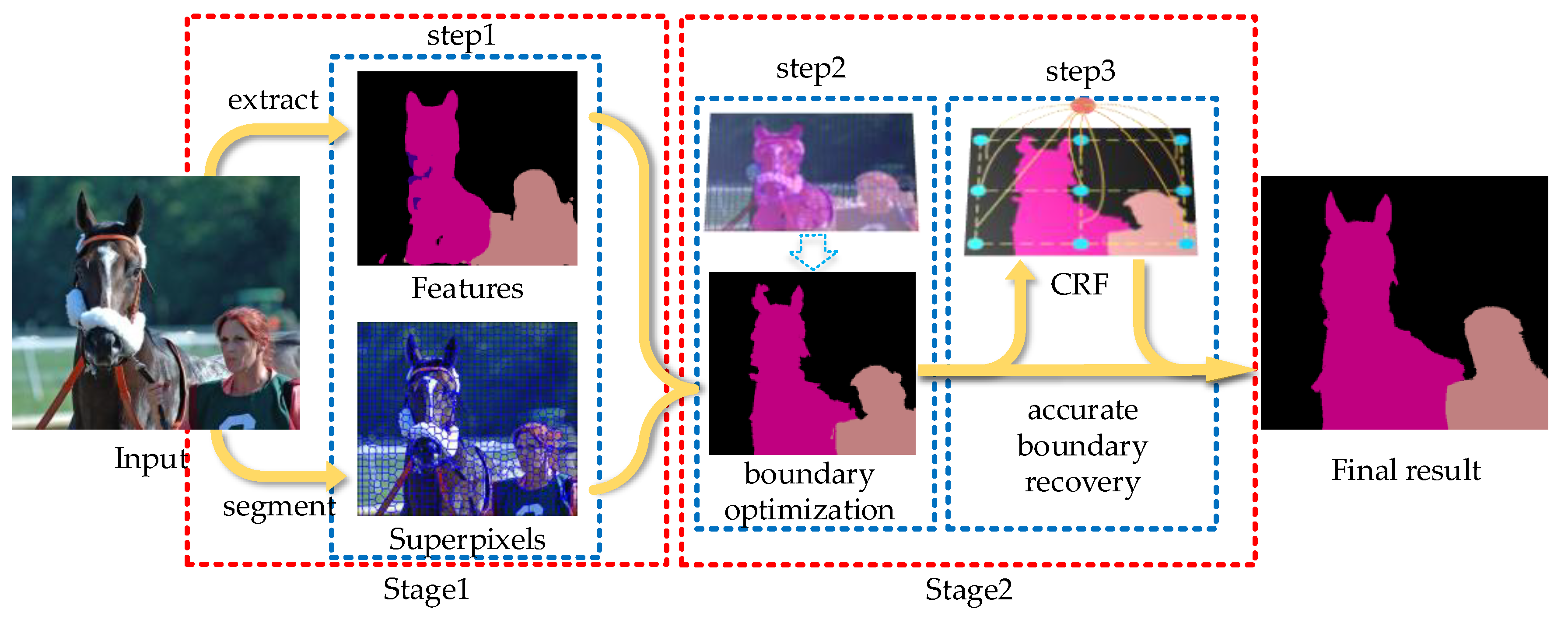
Figure 1 illustrates the flow chart of the proposed method, in which red boxes denote two stages and blue boxes denote three processing steps. In the first step, we use the FCN model to extract the feature information from the input image to obtain pixel-level semantic labels. Although the trained FCN model has fine feature extraction ability, the result is still relatively rough. Meanwhile, the SLIC algorithm is employed to segment the input image and generate a large number of superpixels. In the second step, also the most important, we use coarse features to reassign semantic predictions within each superpixel. Benefiting from the good image boundary adherence of superpixel, we obtain the results of boundary optimization. In the third step, we employ CRFs to predict the semantic label of each pixel for further refining the segmentation boundaries. At this point, the final semantic segmentation result is obtained. Both the high-level semantic information and the low-level cues in image boundaries are fully utilized in our method.
3. Key Techniques
In this section, we describe the theory of feature extraction, boundary optimization, and accurate boundary recovery. The key point is the application of superpixels, which affects the optimization of coarse features and the pixel-by-pixel prediction of CRF model. The technical details are discussed below.
3.1. Feature Extraction
Different from the classic CNN model, the FCN model can take images of arbitrary size as inputs and generate correspondingly-sized outputs, so we employ it to implement the feature extraction in our semantic segmentation method. In this paper, the VGG-based FCN is selected due to its best performance among various structures of FCN model. The VGG-based FCN is transformed from the VGG-16 [28] by replacing the fully connected layers with convolutional ones and keeping the first five layers. After multiple iterations of convolution and pooling, the resolution of the resulting feature map gets lower and lower. Upsampling is required to restore the coarse feature to the output image with the same size as the input one. In the implementation procedure, the resolution of the feature maps is reduced by 2, 4, 8, 16, and 32 times, respectively. Then, upsampling the output of the last layer by 32 times can get the result of FCN-32s. Because the large magnification leads to the lack of image details, the results of FCN-32s are not accurate enough. To improve the accuracy, we added more detailed information of the last few layers, and combined them with the output of FCN-32s. By this means, the FCN-16s and the FCN-8s can be derived.
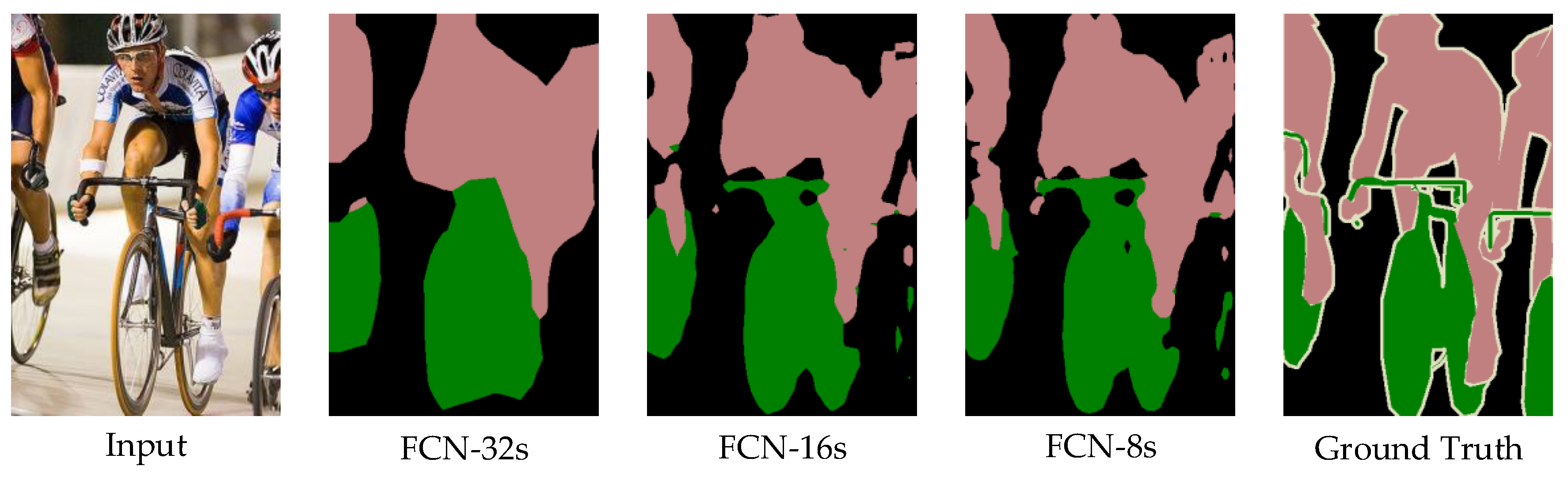
An important problem that needs to be solved in semantic segmentation is how to combine “where” with “what” effectively. In other words, semantic segmentation is to classify pixel-by-pixel and combine the information of position and classification together. On one hand, due to the difference in receptive fields, the resolution is relatively higher in the first few convolutions, and the positioning of the pixels is more accurate. On the other hand, in the last few convolutions, the resolution is relatively lower and the classification of the pixels is more accurate. An example of three models is shown in Figure 2.
It is can be observed from Figure 2 that the result of FCN-32s is drastically smoother and less refined. This is because the receptive field of FCN-32s model is larger and more suitable for macroscopic perception. In contrast, the receptive field of FCN-8s model is smaller and more suitable for feeling the details. From Figure 2 we can also see that the result of FCN-8s, which is closest to the ground truth, is significantly better than those of FCN-16s and FCN-32s. Therefore, we choose FCN-8s as the front-end to extract the coarse features of images. However, the results of FCN-8s are still far from perfect and insensitive to the details of images. In the following, the two-step optimization is introduced in detail.
3.2. Boundary Optimization
In this section, more attention is paid to the optimization of image boundaries. There are some image processing techniques that can be used for the boundary optimization. For example, the method based on graph cut [29] can obtain better edge segmentation results, but it relies on human interactions, which is unacceptable for processing a large number of images. In addition, some edge detection algorithms [30] are often used to optimize the boundary of images. These algorithms share the common feature that the parameters for a particular occasion are fixed, which are more applicable to some specific applications. However, when solving general border tracing problems for images containing unknown objects and backgrounds, the fixed parameter approach often fails to achieve the best results. In this work, superpixel is selected for the boundary optimization purpose. Generally, a superpixel can be treated as a set of pixels that are similar in location, color, texture, etc. According to this similarity, superpixels have a certain visual significance in comparison with pixels. Although a single superpixel has no valid semantic information, it is a part of an object that has semantic information. Besides, the most important property of superpixels is its ability to adhere to image boundaries. Based on this property, superpixels are applied to optimize the coarse features extracted by the front end.
As shown in Figure 3, SLIC is used to generate superpixels, and then the coarse features are optimized by the object boundaries from these superpixels. To some degree, this method can improve the segmentation accuracy of the object boundaries. The critical algorithm of boundary optimization is completely demonstrated in Algorithm 1.
Figure 4 shows the result of boundary optimization by applying Algorithm 1. As can be seen from the partial enlarged details in Figure 4, the edge information of superpixels is utilized effectively, and thus a more accurate result can be obtained.
It is observed from the red box in Figure 4 that a number of superpixels with sharp, smooth, and prominent edges adhere the boundaries of object well. Due to diffusion errors in the upsampling process, a few pixels inside these superpixels have different semantic information. A common mistake is to misclassify background pixels as another classification. Figure 4 shows that this kind of mistake can be corrected effectively using our optimization algorithm. There are some other superpixels with more types of semantic information, while the number of pixels with different classification is about the same. These superpixels can be found in the weak edges or thin structures of images, which are easy to misclassify in a complex environment. For these superpixels, we keep the segmentation results with those delivered by the front end.
| Algorithm 1. The algorithm of boundary optimization. |
|
3.3. Accurate Boundary Recovery
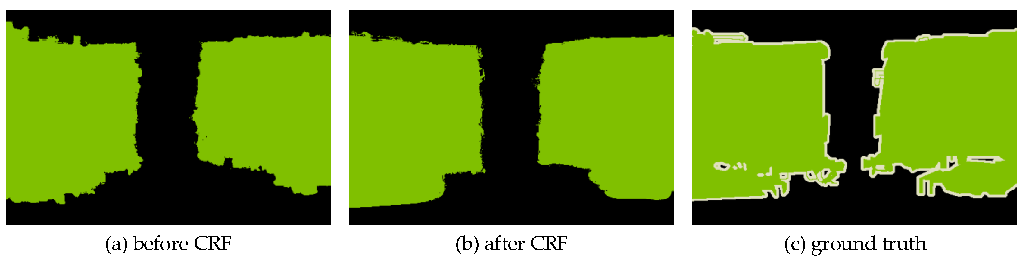
After the above boundary optimization, it is still necessary to improve the segmentation accuracy of the thin structure, weak edge, and complex superposition. Therefore, we employ the CRF model to recover the boundaries more accurately, i.e., to further optimization. To clearly show the effect of the CRF model, an example is given in Figure 5.
Consider the pixel-wise labels as random variables and the relationship between pixels as edges, and correspondingly constitute a conditional random field. These labels can be modelled after we obtain global observations, which are usually the input images. In detail, a global observation is represented as the input image of N pixels in our method. Then, given a graph , and denotes the vertices and the edges of the graph, respectively. Let be the vector formed by the random variables , in which is the random variable representing the label assigned to the pixel . A conditional random field conforms to Gibbs distribution, and the pair can be modelled as
in which E(x) is the Gibbs energy of a labeling and Z(I) is the partition function [31]. The fully connected CRF model [32] employs the energy function
in which is the unary potentials that represent the probability of the pixel taking the label , and is the pairwise potentials that represent the cost of assigning labels , to pixels , at the same time. In our method, the unary potentials can be treated as the boundary optimized feature map that can help improve the performance of CRF model. The pairwise potentials usually model the relationship among neighboring pixels and are weighted by color similarity. The expression is employed for pairwise potentials [32] as shown below:
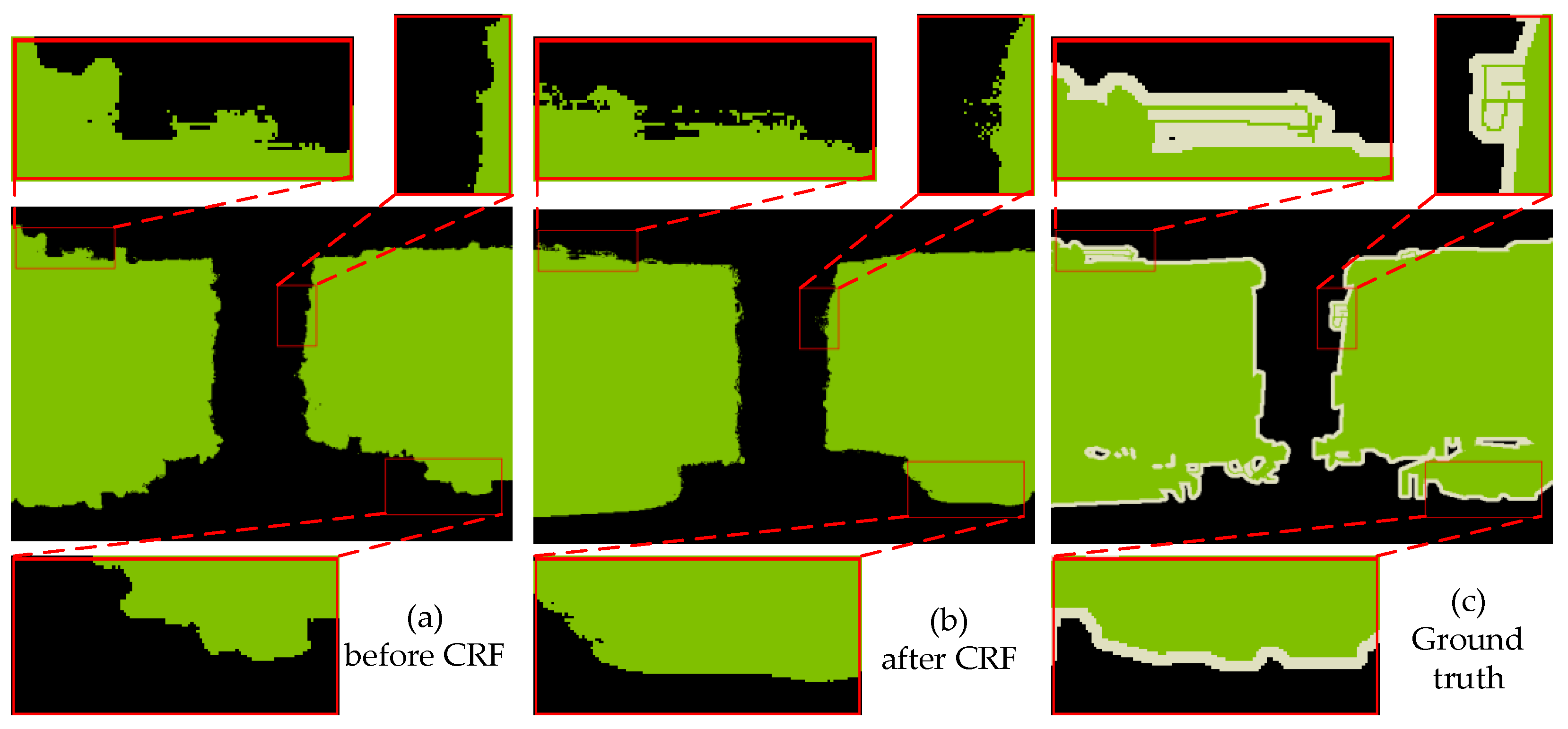
in which the first term depends on both pixel positions and pixel color intensities, and the second term only depends on pixel positions. , are the color vectors, and , are the pixel positions. The other parameters are described in the previous work [32]. As shown in the Potts model [33], is equal to 1 if , and 0 otherwise. It means that nearby similar pixels assigned different labels should be penalized. In other words, similar pixels are encouraged to be assigned the same label, whereas pixels that differ greatly in “distance” are assigned different labels. The definition of “distance” is related to the color and the actual distance; thus, the CRF can segment images at the boundary as much as possible. Partial enlarged details shown in Figure 6 are used to explain the analysis of the accurate boundary recovery.
4. Experimental Evaluation
In this section, we first describe the used experimental setup, including the datasets and the selection of parameters. Next, we provide comprehensive ablation study of each component of the improved method. Then, the evaluation of the proposed method is given, together with other state-of-the-art methods. Qualitative and quantitative experimental results are presented entirely, and necessary comparisons are performed to validate the competitive performance of our method.
4.1. Experimental Setup
We use the PASCAL VOC 2012 segmentation benchmark [34], as it has become the standard dataset to comprehensively evaluate any new semantic segmentation methods. It involves 20 foreground classes and one background class. For our experiments on VOC 2012, we adopt the extended training set of 10,581 images [35] and a reduced validation set of 346 images [20]. We further evaluate the improved method on the Cityscapes dataset [36], which focuses on semantic understanding of urban street scenes. It consists of around 5000 fine annotated images of street scenes and 20,000 coarse annotated ones, in which all annotations are from 19 semantic classes.
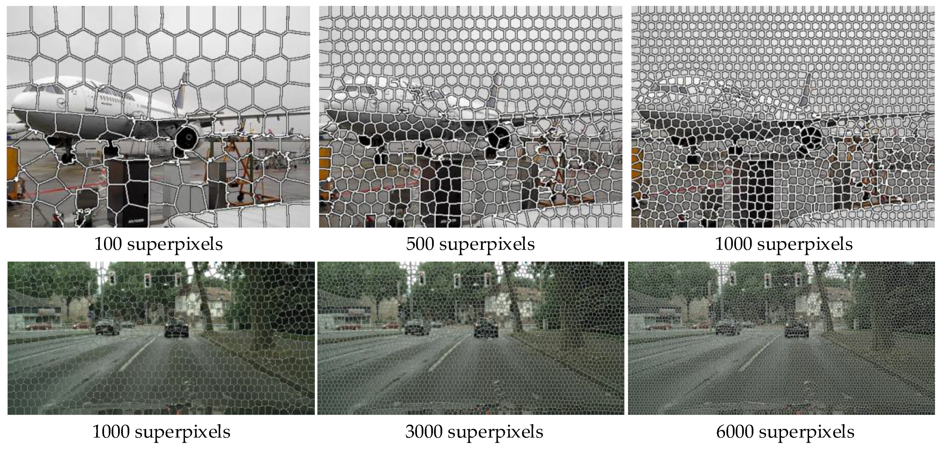
From Figure 7, it can be seen that as the number of superpixels increases; a single superpixel will get closer to the edge of the object. Most of images in VOC dataset have a resolution of around , so we set the number of superpixels to 1000. For Cityscapes dataset, we set the number of superpixels to 6000 due to the high-resolution of images. In our experiments, 10 mean field iterations are employed for CRF. Meanwhile, we use default values of and set , and by the same strategy in [22].
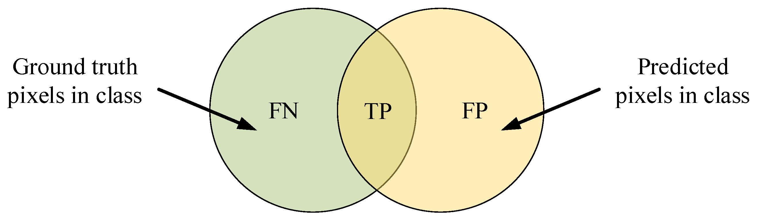
The standard Jaccard Index (Figure 8), also known as the PASCAL VOC intersection-over-union (IoU) metric [34], is introduced for the performance assessment in this paper:
According to Jaccard Index, many evaluation criteria have been proposed to evaluate the segmentation accuracy. Among them, PA, IoU, and mIoU are often used, and their definitions can be found in the previous work [37]. We assume a total of k + 1 classes (including a background class), and is the amount of pixels of class inferred to class . represents the number of true positives, while and are usually interpreted as false positives and false negatives, respectively. The formulas of PA, IoU, and mIoU are shown below:
● Pixel Accuracy (PA):
which computes a ratio between the number of properly classified pixels and the total number of them.
● Intersection Over Union (IoU):
which is used to measure whether the target in the image is detected.
● Mean Intersection Over Union (mIoU):
which is the standard metric for segmentation purposes and computed by averaging IoU. mIoU computes a ratio between the ground truth and our predicted segmentation.
4.2. Ablation Study
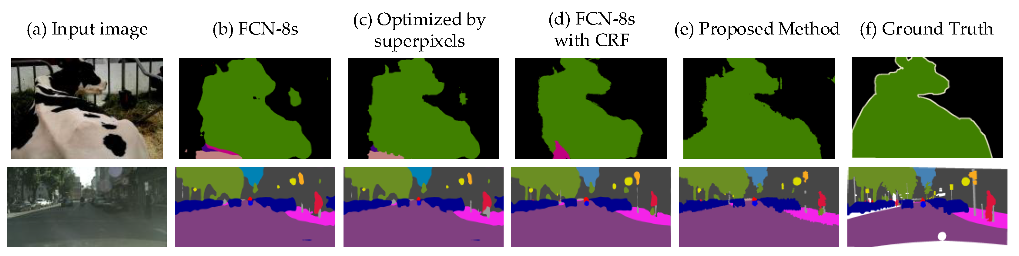
The core idea of the improved method lies in the utility of superpixels and the optimization of CRF model. First, to evaluate the importance of the utility of superpixels, we directly compared the plain FCN-8s model with the boundary optimized one. Then, the FCN-8s with CRF and our proposed method are implemented sequentially. For better understanding, the results of these comparative experiments are shown in Figure 9 and Table 1.
From the results, we see that methods with boundary optimization by superpixels consistently perform better than the counterparts without optimization. For example, as shown in Table 1, the method with boundary optimization is 3.2% better than the plain FCN-8s on VOC dataset, while the improvement becomes 2.8% on Cityscapes dataset. It can be observed that the object boundaries in Figure 9c are closer to the ground truth than Figure 9b. Based on the above experimental results, we can conclude that the segmentation accuracy of the object boundaries can be improved by the utility of superpixels. Table 1 also shows that, for the FCN-8s with CRF applied as a post-processing step, the better performance can be observed after boundary optimization. As shown in Figure 9d,e, the results of our method are more similar with the ground truth than that without boundary optimization. The mIoU scores of the two right-most columns also corroborated this point, with an improvement of 5% on VOC dataset and 4.1% on Cityscapes dataset.
The purpose of using CRFs is to recover the boundaries more accurately. We compared the performance of plain FCN-8s with/without CRF under the same situation. From Table 1, it is clear that CRF consistently boosts classification scores on both the VOC dataset and the Cityscapes dataset. Besides, we compared the performance of boundary optimized FCN-8s with/without CRF. In conclusion, methods optimized by CRFs outperform the counterparts by a significant margin, which shows the importance of boundary optimization and CRFs.
4.3. Experimental Results
4.3.1. Qualitative Analysis
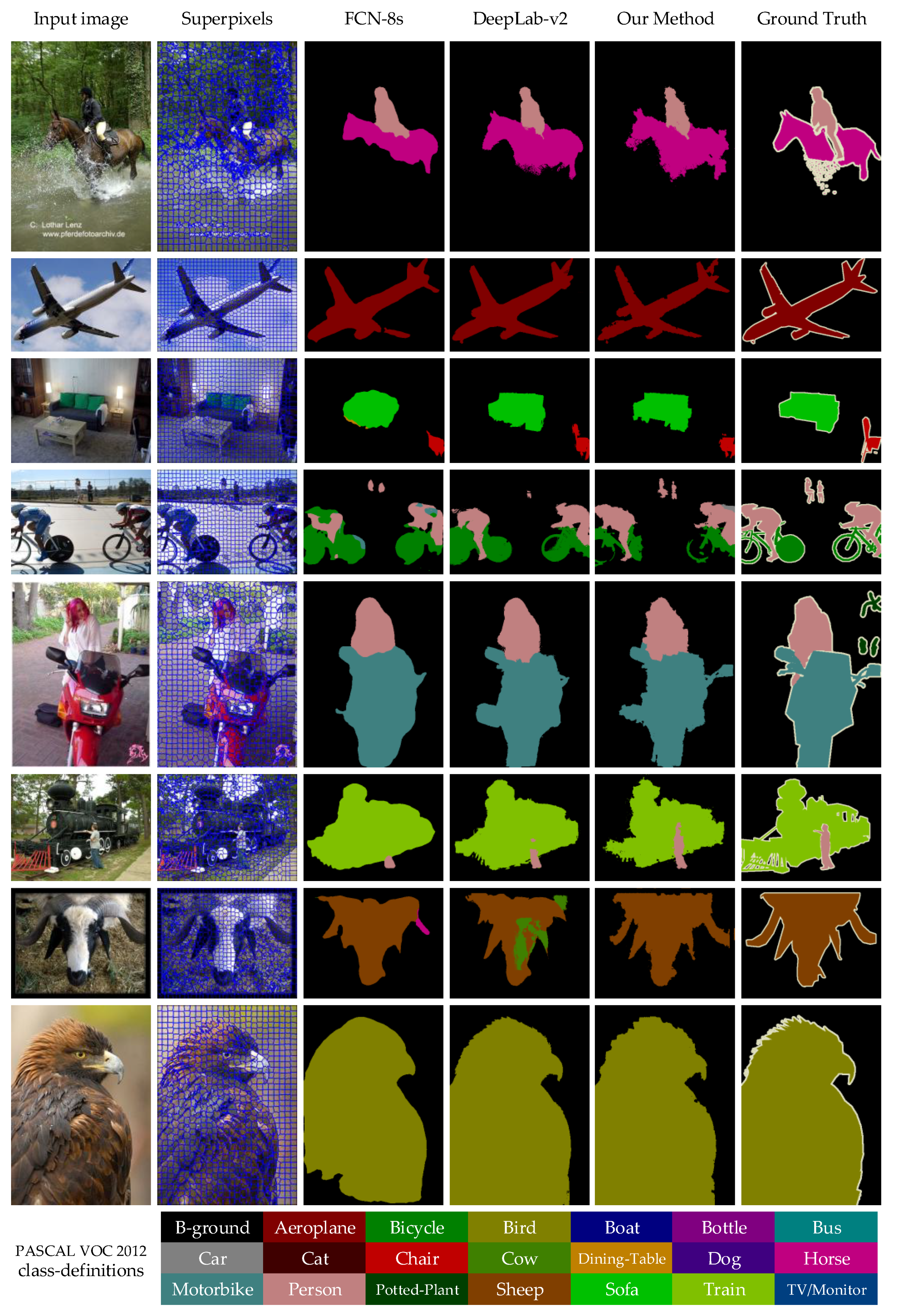
According to the method proposed in this paper, we have obtained the improved semantic segmentation results. The comparisons on VOC dataset among FCN-8s, DeepLab-v2 [22], and our method are shown in Figure 10.
As shown in Figure 10, our results are significantly closer to the ground truth than those by FCN-8s, especially for the segmentation of the object edges in images. By comparing the results obtained by FCN-8s with ours, it can be seen that they are the same color and they have a similar object outline, which indicates that our method inherits feature extraction and object recognition abilities of FCN. In addition, our method can get finer details than DeepLab-v2 in the vast majority of categories, which profits from the boundary optimization of coarse features. From segmentation results of each image in Figure 10, we also notice the following details: (a) All these methods can identify the classification of the single large object and locate the region accurately, due to the excellent extraction ability of CNNs. (b) In the complex scene, these methods cannot work effectively due to the error of extracted features, even employing different post-processing steps. (c) Small objects are possible to be misidentified or missed, due to the lack of the pixels describing the small objects.
It is worth mentioning that, in some details of Figure 10, such as the rear wheel of the first bicycle, the results of DeepLab-v2 seem better than ours. The segmentation result of DeepLab-v2 almost completely retained the rear wheel of the first bicycle. However, it cannot be overlooked that DeepLab-v2 fails to properly process the front wheels of the two bicycles. In contrast, the front wheels processed by our method are closer to that of ground truth. For the rear wheel missing problem, some analysis is made on the difference among the bicycle body, solid rear wheel, and background. The solid rear wheel has a distinguished color with compassion of the background, but at the same time, the same case exists in the bicycle body and solid rear wheel, leading to a large probability of misrecognition. Additionally, the non-solid wheel is much more common than the solid one in the real scenario; therefore, the CRF model tends to predict the non-solid wheel.
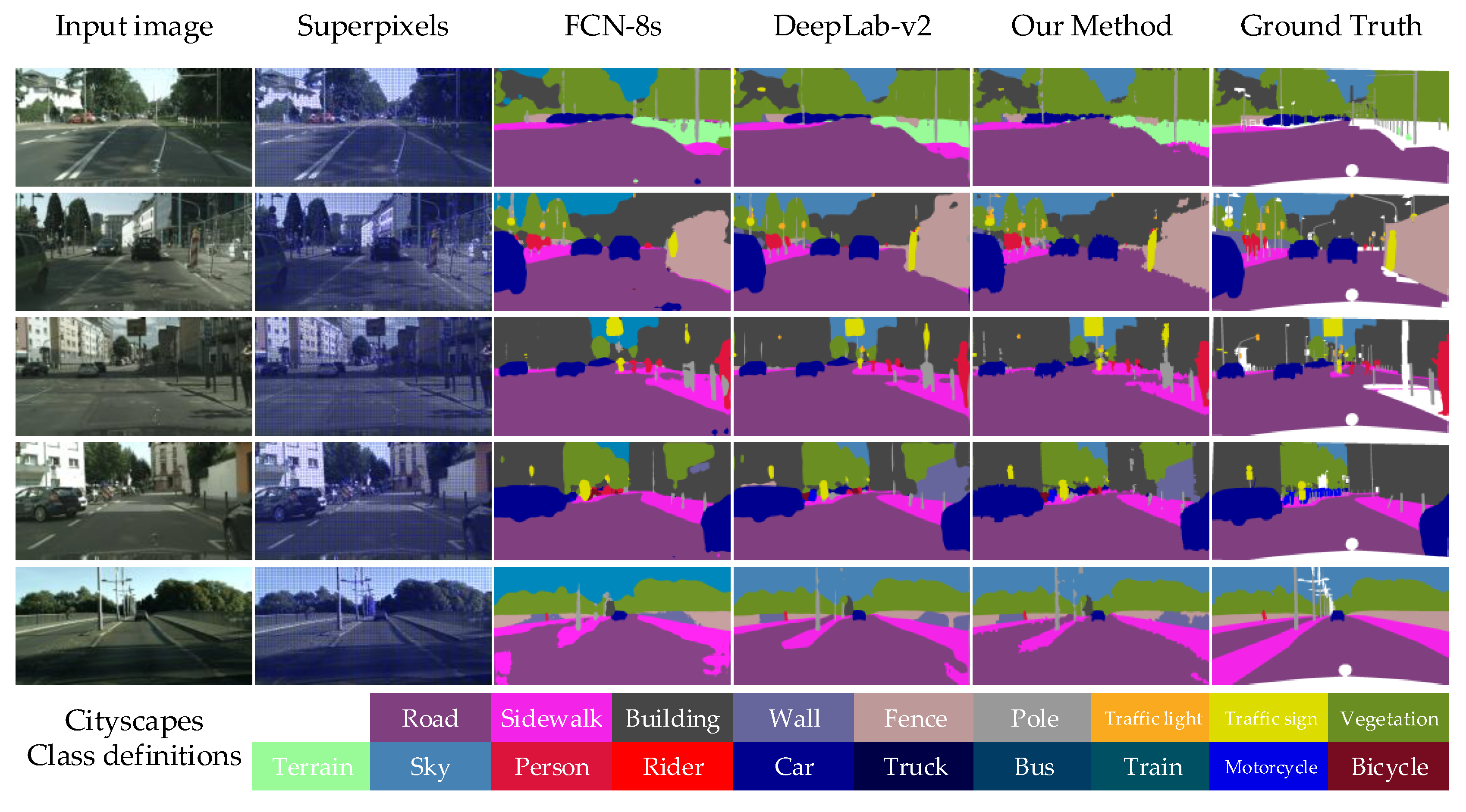
The proposed semantic segmentation method is implemented on Cityscapes dataset. Some visual results proposed by FCN-8s, DeepLab-v2, and our method are shown in Figure 11. Similar to the results on PASCAL VOC 2012 dataset, the improved method achieves better performance than others.
4.3.2. Quantitative Analysis
● PASCAL VOC 2012 Dataset
The per-class IoU scores on VOC dataset among FCN-8s, the proposed method, and other popular methods are shown in Table 2. It can be observed that our method achieves the best performance in most categories, which is consistent with the conclusion obtained in qualitative analysis. In addition, the proposed method outperforms prior methods in mIoU metric; it reaches the highest 74.5% accuracy.
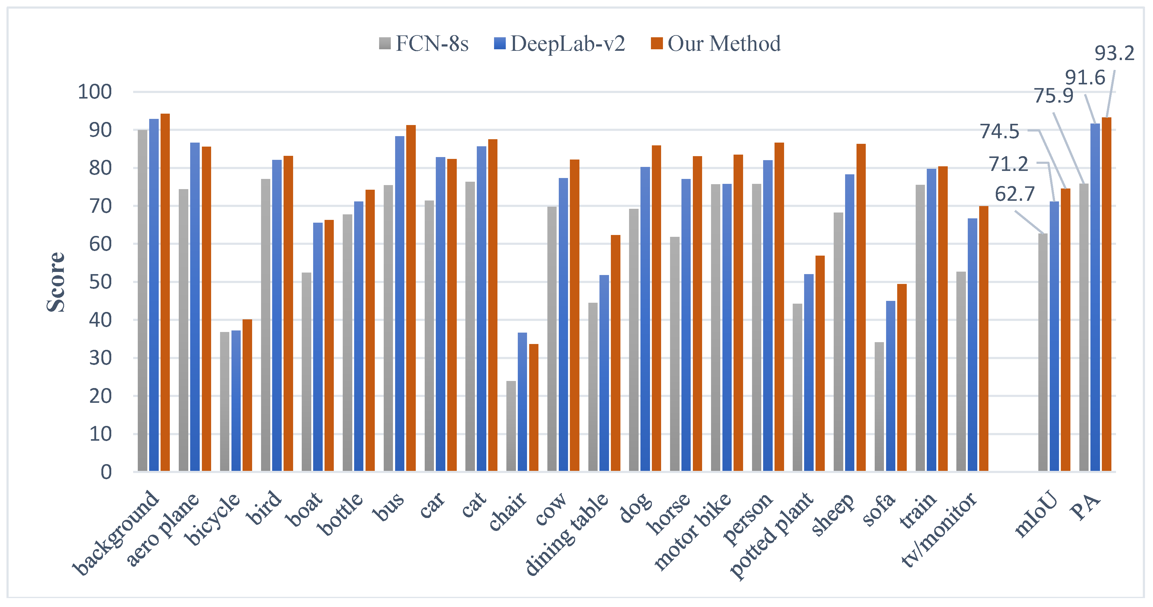
This work proposed a post-processing method to improve the FCN-8s result. During the implementation procedure, the superpixel and the CRF are used subsequently to improve the coarse results extracted by FCN-8s. Therefore, the comparison with FCN-8s is the most primary and direct way to illustrate the improvement level of our method. Meanwhile, to further evaluate the performance of our method, the comparison with DeepLab has been made. The IoU, mIoU, and PA scores of FCN-8s and DeepLab-v2, and our methods are given in Figure 12.
It can be observed from Figure 12, compared with FCN-8s, that the proposed method significantly improves the IoU score in every category with higher mIoU and PA scores. In addition, our method is better than DeepLab-v2 in most categories (except for aero plane, car and chair). The detailed improvement statistics are shown in Figure 13.
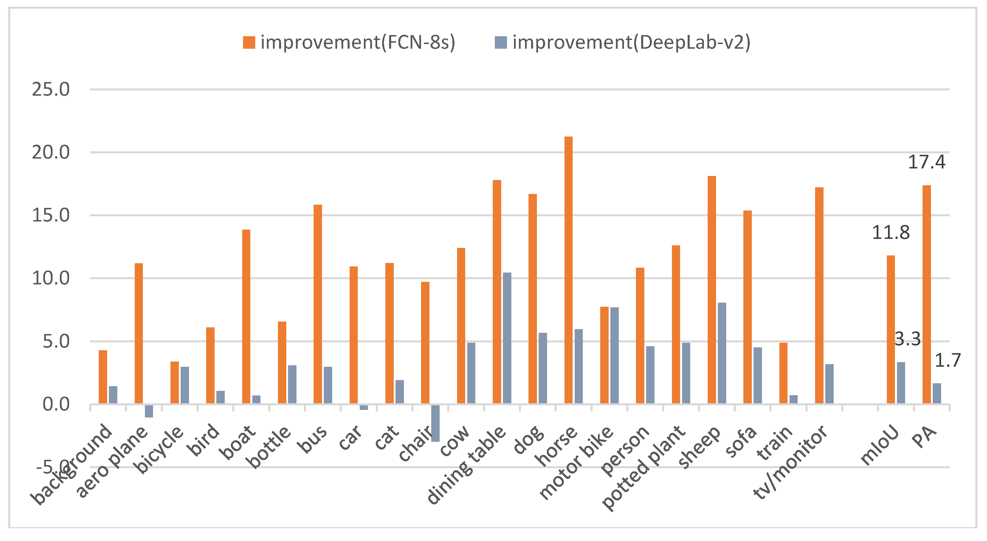
As shown in Figure 13, our method can be significantly improved compared with FCN-8s, which reach up to 11.8% in mIoU and 17.4% in PA, respectively. For DeepLab-v2, the improvements of mIoU and PA are 3.3% and 1.7%. Moreover, Figure 13 intuitively shows the improvement level using our method in comparison with FCN-8s and DeepLab. The improvement can be clearly observed in 100% (21/21) of categories when compared with FCN-8s. Meanwhile, there is 85.71% (18/21) of categories improvement in comparison withDeepLab-v2. In summary, our method achieved the best performance among these three methods.
● Cityscapes Dataset
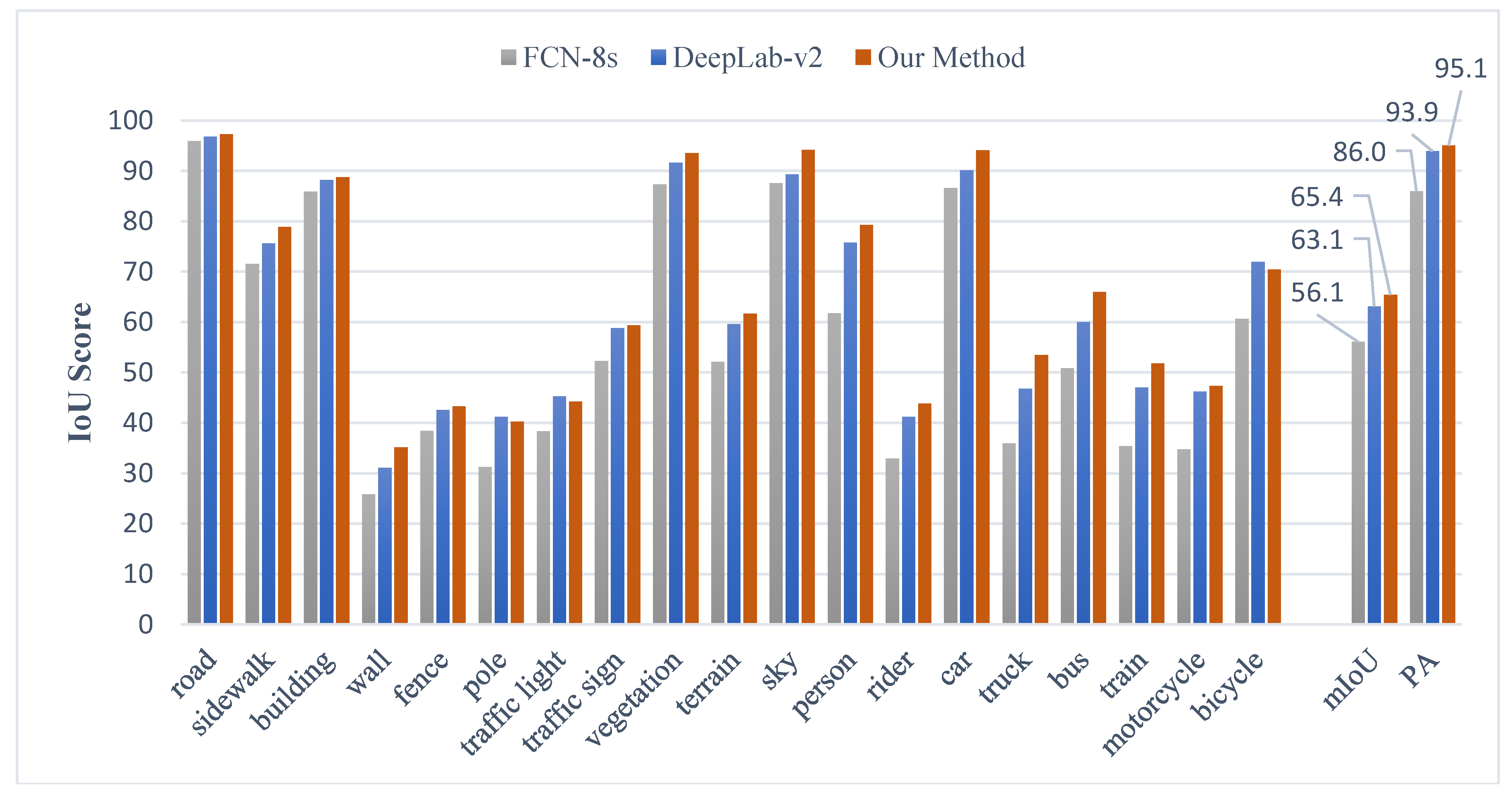
We conducted an experiment on the Cityscapes dataset, which differs from the previous one in the high-resolution images and the number of classes. We used the provided partitions of training and validation sets, and the obtained results are reported in Table 3. It can be observed that the evaluation on the Cityscapes validation set is similar to that on the VOC dataset. Using our method, the highest mIoU score can reach up to 65.4%. The IoU, mIoU, and PA scores of FCN-8s, DeepLab-v2, and our method are given in Figure 14.
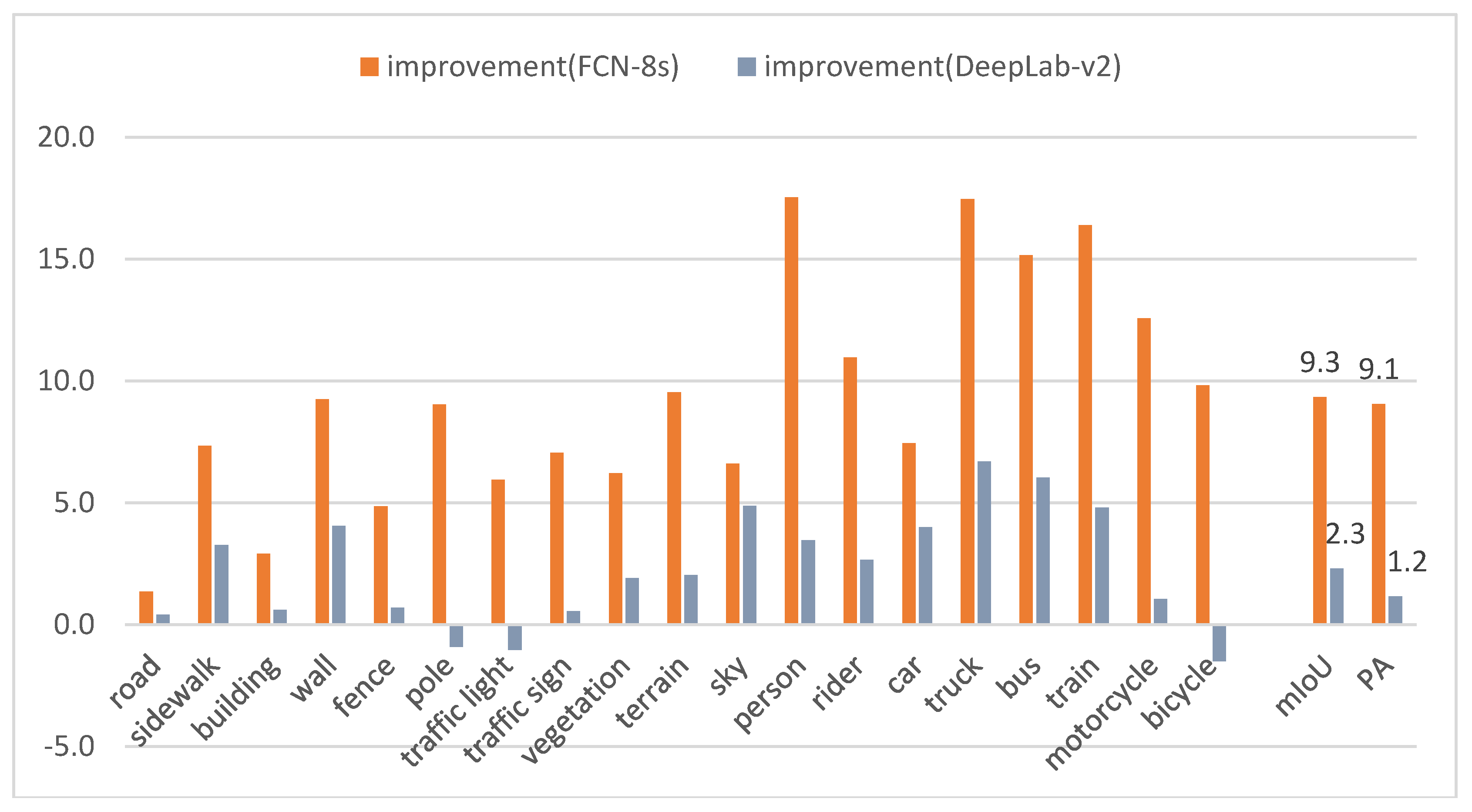
It can be observed from Figure 14 that the proposed method has significantly improved the IoU, mIoU, and PA scores in every category with the comparison of FCN-8s. Similar to the results in VOC 2012 dataset, our method is better than DeepLab-v2 in most categories (except for pole, traffic light, and bicycle). The detailed improvement statistics are shown in Figure 15.
As shown in Figure 15, our method can get a significant improvement compared with FCN-8s, which reach up to 9.3% in mIoU and 9.1% in PA, respectively. Moreover, Figure 15 intuitively shows the improvement level using our method with the comparison of FCN-8s and DeepLab-v2. The improvement can be clearly observed in 100% (19/19) of categories when compared with FCN-8s and 84.21% (16/19) of categories when compared with DeepLab-v2, respectively.
5. Conclusions
In this paper, an improved semantic segmentation method is proposed, which utilizes the superpixel edges of images and the constraint relationship between different pixels. First, our method has the ability to extract advanced semantic information, which is inherited from the FCN model. Then, to effectively optimize the boundaries of results, our method takes into account the good adherence to the edges of superpixels. Finally, we apply CRF to further predict the semantic information of each pixel, and make full use of the local texture features of the image, global context information, and smooth priori. Experiment results show that our method can achieve the more accurate segmentation result. Using our method, mIoU scores can reach up to 74.5% on the VOC dataset and 65.4% on the Cityscapes dataset, which are 11.8% and 9.3% improvements over FCN-8s, respectively.
Author Contributions
Hai Wang, Wei Zhao, and Yi Fu conceived and designed the experiments; Yi Fu and Xiaosong Wei performed the experiments; Wei Zhao and Yi Fu analyzed the data; Xiaosong Wei contributed analysis tools; Hai Wang, Wei Zhao, and Yi Fu wrote the paper.
Conflicts of Interest
The authors declare no conflict of interest.
References
- Oberweger, M.; Wohlhart, P.; Lepetit, V. Hands deep in deep learning for hand pose estimation. arXiv, 2015; arXiv:1502.06807. [Google Scholar]
- Geiger, A.; Lenz, P.; Urtasun, R. Are we ready for autonomous driving? The kitti vision benchmark suite. In Proceedings of the 2012 IEEE Conference on Computer Vision and Pattern Recognition, Providence, RI, USA, 16–21 June 2012; IEEE: New York, NY, USA, 2012; pp. 3354–3361. [Google Scholar]
- Wan, J.; Wang, D.; Hoi, S.C.H.; Wu, P.; Zhu, J.; Zhang, Y.; Li, J. Deep learning for content-based image retrieval: A comprehensive study. In Proceedings of the 22nd ACM International Conference on Multimedia, Orlando, FL, USA, 3–7 November 2014; ACM: Orlando, FL, USA, 2014; pp. 157–166. [Google Scholar]
- Kang, W.X.; Yang, Q.Q.; Liang, R.P. The comparative research on image segmentation algorithms. In Proceedings of the 2009 First International Workshop on Education Technology and Computer Science, Wuhan, China, 7–8 March 2009; pp. 703–707. [Google Scholar]
- Ciresan, D.; Giusti, A.; Gambardella, L.M.; Schmidhuber, J. Deep neural networks segment neuronal membranes in electron microscopy images. In Proceedings of the Advances in Neural Information Processing Systems 25, Lake Tahoe, NV, USA, 3–6 December 2012; Curran Associates, Inc.: Red Hook, NY, USA, 2012; pp. 2843–2851. [Google Scholar]
- Gupta, S.; Girshick, R.; Arbeláez, P.; Malik, J. Learning rich features from rgb-d images for object detection and segmentation. In European Conference on Computer Vision; Springer: New York, NY, USA, 2014; pp. 345–360. [Google Scholar]
- Hariharan, B.; Arbeláez, P.; Girshick, R.; Malik, J. Simultaneous detection and segmentation. In European Conference on Computer Vision; Springer: New York, NY, USA, 2014; pp. 297–312. [Google Scholar]
- Girshick, R.; Donahue, J.; Darrell, T.; Malik, J. Rich feature hierarchies for accurate object detection and semantic segmentation. In Proceedings of the 2014 IEEE Conference on Computer Vision and Pattern Recognition, Columbus, OH, USA, 24–27 June 2014; IEEE Computer Society: Washington, DC, USA, 2014; pp. 580–587. [Google Scholar]
- Ren, S.; He, K.; Girshick, R.; Sun, J. Faster r-cnn: Towards real-time object detection with region proposal networks. IEEE Trans. Pattern Anal. Mach. Intell. 2017, 39, 1137–1149. [Google Scholar] [CrossRef] [PubMed]
- Luo, P.; Wang, G.; Lin, L.; Wang, X. Deep dual learning for semantic image segmentation. In Proceedings of the IEEE Conference on Computer Vision and Pattern Recognition, Honolulu, HI, USA, 21–26 July 2017; pp. 2718–2726. [Google Scholar]
- Zhao, H.; Shi, J.; Qi, X.; Wang, X.; Jia, J. Pyramid scene parsing network. In Proceedings of the IEEE Conference on Computer Vision and Pattern Recognition (CVPR), Honolulu, HI, USA, 21–26 July 2017; pp. 2881–2890. [Google Scholar]
- Ravì, D.; Bober, M.; Farinella, G.M.; Guarnera, M.; Battiato, S. Semantic segmentation of images exploiting dct based features and random forest. Pattern Recogn. 2016, 52, 260–273. [Google Scholar] [CrossRef]
- Fu, J.; Liu, J.; Wang, Y.; Lu, H. Stacked deconvolutional network for semantic segmentation. arXiv, 2017; arXiv:1708.04943. [Google Scholar]
- Wu, Z.; Shen, C.; Hengel, A.V.D. Wider or deeper: Revisiting the resnet model for visual recognition. arXiv, 2016; arXiv:1611.10080. [Google Scholar]
- Long, J.; Shelhamer, E.; Darrell, T. Fully convolutional networks for semantic segmentation. In Proceedings of the 2015 IEEE Conference on Computer Vision and Pattern Recognition, Boston, MA, USA, 8–10 June 2015; IEEE: New York, NY, USA, 2015; pp. 3431–3440. [Google Scholar]
- Ghiasi, G.; Fowlkes, C.C. Laplacian pyramid reconstruction and refinement for semantic segmentation. In Proceedings of the European Conference on Computer Vision, Amsterdam, The Netherlands, 8–16 October 2016; Springer: New York, NY, USA, 2016; pp. 519–534. [Google Scholar]
- Lin, G.; Shen, C.; Hengel, A.V.D.; Reid, I. Exploring context with deep structured models for semantic segmentation. IEEE Trans. Pattern Anal. Mach. Intell. 2018, 40, 1352–1366. [Google Scholar] [CrossRef] [PubMed]
- Noh, H.; Hong, S.; Han, B. Learning deconvolution network for semantic segmentation. In Proceedings of the IEEE International Conference on Computer Vision, Boston, MA, USA, 8–10 June 2015; pp. 1520–1528. [Google Scholar]
- Chen, L.C.; Yang, Y.; Wang, J.; Xu, W.; Yuille, A.L. Attention to scale: Scale-aware semantic image segmentation. In Proceedings of the 2016 IEEE Conference on Computer Vision and Pattern Recognition, Las Vegas, NV, USA, 27 June–1 July 2016; IEEE: New York, NY, USA, 2016; pp. 3640–3649. [Google Scholar]
- Zheng, S.; Jayasumana, S.; Romera-Paredes, B.; Vineet, V.; Su, Z.Z.; Du, D.L.; Huang, C.; Torr, P.H.S. Conditional random fields as recurrent neural networks. In Proceedings of the 2015 IEEE International Conference on Computer Vision, Santiago, Chile, 7–13 December 2015; IEEE: New York, NY, USA, 2015; pp. 1529–1537. [Google Scholar]
- Chen, L.-C.; Papandreou, G.; Kokkinos, I.; Murphy, K.; Yuille, A.L. Semantic image segmentation with deep convolutional nets and fully connected crfs. arXiv, 2014; arXiv:1412.7062. [Google Scholar]
- Chen, L.C.; Papandreou, G.; Kokkinos, I.; Murphy, K.; Yuille, A.L. Deeplab: Semantic image segmentation with deep convolutional nets, atrous convolution, and fully connected crfs. IEEE Trans. Pattern Anal. Mach. Intell. 2018, 40, 834–848. [Google Scholar] [CrossRef] [PubMed]
- Chen, L.-C.; Papandreou, G.; Schroff, F.; Adam, H. Rethinking atrous convolution for semantic image segmentation. arXiv, 2017; arXiv:1706.05587. [Google Scholar]
- Shi, J.; Malik, J. Normalized cuts and image segmentation. IEEE Trans. Pattern Anal. Mach. Intell. 2000, 22, 888–905. [Google Scholar]
- Felzenszwalb, P.F.; Huttenlocher, D.P. Efficient graph-based image segmentation. Int. J. Comput. Vis. 2004, 59, 167–181. [Google Scholar] [CrossRef]
- Van den Bergh, M.; Boix, X.; Roig, G.; de Capitani, B.; Van Gool, L. Seeds: Superpixels extracted via energy-driven sampling. In Proceedings of the 12th European Conference on Computer Vision-Volume Part VII, Florence, Italy, 7–13 October 2012; Springer: New York, NY, USA, 2012; pp. 13–26. [Google Scholar]
- Achanta, R.; Shaji, A.; Smith, K.; Lucchi, A.; Fua, P.; Susstrunk, S. Slic superpixels compared to state-of-the-art superpixel methods. IEEE Trans. Pattern Anal. Mach. Intell. 2012, 34, 2274–2281. [Google Scholar] [CrossRef] [PubMed]
- Simonyan, K.; Zisserman, A. Very deep convolutional networks for large-scale image recognition. arXiv, 2014; arXiv:1409.1556. [Google Scholar]
- Rother, C.; Kolmogorov, V.; Blake, A. Grabcut: Interactive foreground extraction using iterated graph cuts. In Proceedings of the ACM Transactions on Graphics (TOG), Los Angeles, CA, USA, 8–12 August 2004; ACM: New York, NY, USA, 2004; Volume 23, pp. 309–314. [Google Scholar]
- Maini, R.; Aggarwal, H. Study and comparison of various image edge detection techniques. Int. J. Image Process. 2009, 3, 1–11. [Google Scholar]
- Gadde, R.; Jampani, V.; Kiefel, M.; Kappler, D.; Gehler, P.V. Superpixel convolutional networks using bilateral inceptions. In Computer Vision, ECCV 2016; Leibe, B., Matas, J., Sebe, N., Welling, M., Eds.; Springer International Publishing: Cham, Switzerland, 2016; Volume 9905, pp. 597–613. [Google Scholar]
- Krähenbühl, P.; Koltun, V. Efficient inference in fully connected crfs with gaussian edge potentials. In Proceedings of the 24th International Conference on Neural Information Processing Systems, Granada, Spain, 12–15 December 2011; Curran Associates Inc.: Red Hook, NY, USA, 2011; pp. 109–117. [Google Scholar]
- Wu, F. The potts model. Rev. Mod. Phys. 1982, 54, 235. [Google Scholar] [CrossRef]
- Everingham, M.; Eslami, S.M.A.; Van Gool, L.; Williams, C.K.I.; Winn, J.; Zisserman, A. The pascal visual object classes challenge: A retrospective. Int. J. Comput. Vis. 2015, 111, 98–136. [Google Scholar] [CrossRef]
- Hariharan, B.; Arbelaez, P.; Bourdev, L.; Maji, S.; Malik, J. Semantic contours from inverse detectors. In Proceedings of the 2011 International Conference on Computer Vision, Barcelona, Spain, 6–13 November 2011; IEEE Computer Society: Washington, DC, USA, 2011; pp. 991–998. [Google Scholar]
- Cordts, M.; Omran, M.; Ramos, S.; Scharwächter, T.; Enzweiler, M.; Benenson, R.; Franke, U.; Roth, S.; Schiele, B. The cityscapes dataset. In Proceedings of the CVPR Workshop on the Future of Datasets in Vision, Boston, MA, USA, 11 June 2015; p. 3. [Google Scholar]
- Garcia-Garcia, A.; Orts-Escolano, S.; Oprea, S.; Villena-Martinez, V.; Garcia-Rodriguez, J. A review on deep learning techniques applied to semantic segmentation. arXiv, 2017; arXiv:1704.06857. [Google Scholar]
- Mostajabi, M.; Yadollahpour, P.; Shakhnarovich, G. Feedforward semantic segmentation with zoom-out features. In Proceedings of the IEEE Conference on Computer Vision and Pattern Recognition, Boston, MA, USA, 7–12 June 2015; pp. 3376–3385. [Google Scholar]
- Vemulapalli, R.; Tuzel, O.; Liu, M.-Y.; Chellapa, R. Gaussian conditional random field network for semantic segmentation. In Proceedings of the IEEE Conference on Computer Vision and Pattern Recognition, Las Vegas, NV, USA, 27 June–1 July 2016; pp. 3224–3233. [Google Scholar]
- Liu, Z.; Li, X.; Luo, P.; Loy, C.-C.; Tang, X. Semantic image segmentation via deep parsing network. In Proceedings of the 2015 IEEE International Conference on Computer Vision (ICCV), Santiago, Chile, 7–13 December 2015; IEEE: New York, NY, USA, 2015; pp. 1377–1385. [Google Scholar]
Figure 1.
The flow chart of the proposed method.

Figure 2.
The features extracted from FCN models.

Figure 3.
Boundary optimization using superpixels.

Figure 4.
Boundary optimization and partial enlarged details.

Figure 5.
An example of before/after CRF.

Figure 6.
Accurate boundary recovery and partial enlarged details.

Figure 7.
Results with different superpixel number. The first row: SLIC segmentation results with 100, 500, and 1000 superpixels on an example image in VOC dataset. The second row: SLIC segmentation results with 1000, 3000, and 6000 superpixels on an example image in Cityscapes dataset.
Figure 7.
Results with different superpixel number. The first row: SLIC segmentation results with 100, 500, and 1000 superpixels on an example image in VOC dataset. The second row: SLIC segmentation results with 1000, 3000, and 6000 superpixels on an example image in Cityscapes dataset.

Figure 8.
The standard Jaccard Index, in which TP, FP, and FN are the numbers of true positive, false positive, and false negative pixels.
Figure 8.
The standard Jaccard Index, in which TP, FP, and FN are the numbers of true positive, false positive, and false negative pixels.

Figure 9.
An example result of the comparative experiments. (a) The input image, (b) the result of plain FCN-8s, (c) the boundary optimization result by superpixels, (d) the result of FCN-8s with CRF post-processing, (e) the result of our method, and (f) the ground truth.
Figure 9.
An example result of the comparative experiments. (a) The input image, (b) the result of plain FCN-8s, (c) the boundary optimization result by superpixels, (d) the result of FCN-8s with CRF post-processing, (e) the result of our method, and (f) the ground truth.

Figure 10.
Qualitative results on the reduced validation set of PASCAL VOC 2012. From left to right: the original image, SLIC segmentation, FCN-8s results, DeepLab-v2 results, our results, and the ground truth.
Figure 10.
Qualitative results on the reduced validation set of PASCAL VOC 2012. From left to right: the original image, SLIC segmentation, FCN-8s results, DeepLab-v2 results, our results, and the ground truth.

Figure 11.
Visual results on the validation set of Cityscapes. From left to right: the original image, SLIC segmentation, FCN-8s results, DeepLab-v2 results, our results, and the ground truth.
Figure 11.
Visual results on the validation set of Cityscapes. From left to right: the original image, SLIC segmentation, FCN-8s results, DeepLab-v2 results, our results, and the ground truth.

Figure 12.
IoU, mIoU, and PA scores on the PASCAL VOC 2012 dataset.

Figure 13.
The improvement by our method compared with FCN-8s and DeepLab-v2.

Figure 14.
IoU, mIoU, and PA scores on the Cityscapes dataset.

Figure 15.
The improvement by our method compared with FCN-8s and DeepLab-v2.


Table 1.
The mIoU scores of the comparative experiments.
| DatasetMethod | Plain FCN-8s | With BO 1 | With CRF | Our Method |
|---|---|---|---|---|
| VOC 2012 | 62.7 | 65.9 | 69.5 | 74.5 |
| Cityscapes | 56.1 | 58.9 | 61.3 | 65.4 |
1 BO denotes the Boundary Optimization.
Table 2.
Per-class IoU score on VOC dataset. Best performance of each category is highlighted in bold.
Table 2.
Per-class IoU score on VOC dataset. Best performance of each category is highlighted in bold.
| FCN-8s | Zoom-Out [38] | DeepLab-v2 | CRF-RNN [20] | GCRF [39] | DPN [40] | Our Method | |
|---|---|---|---|---|---|---|---|
| areo | 74.3 | 85.6 | 86.6 | 87.5 | 85.2 | 87.7 | 85.5 |
| bike | 36.8 | 37.3 | 37.2 | 39.0 | 43.9 | 59.4 | 40.1 |
| bird | 77.0 | 83.2 | 82.1 | 79.7 | 83.3 | 78.4 | 83.1 |
| boat | 52.4 | 62.5 | 65.6 | 64.2 | 65.2 | 64.9 | 66.3 |
| bottle | 67.7 | 66.0 | 71.2 | 68.3 | 68.3 | 70.3 | 74.2 |
| bus | 75.4 | 85.1 | 88.3 | 87.6 | 89.0 | 89.3 | 91.3 |
| car | 71.4 | 80.7 | 82.8 | 80.8 | 82.7 | 83.5 | 82.3 |
| cat | 76.3 | 84.9 | 85.6 | 84.4 | 85.3 | 86.1 | 87.5 |
| chair | 23.9 | 27.2 | 36.6 | 30.4 | 31.1 | 31.7 | 33.6 |
| cow | 69.7 | 73.2 | 77.3 | 78.2 | 79.5 | 79.9 | 82.2 |
| table | 44.5 | 57.5 | 51.8 | 60.4 | 63.3 | 62.6 | 62.3 |
| dog | 69.2 | 78.1 | 80.2 | 80.5 | 80.5 | 81.9 | 85.9 |
| horse | 61.8 | 79.2 | 77.1 | 77.8 | 79.3 | 80.0 | 83.0 |
| mbike | 75.7 | 81.1 | 75.7 | 83.1 | 85.5 | 83.5 | 83.4 |
| person | 75.7 | 77.1 | 82.0 | 80.6 | 81.0 | 82.3 | 86.6 |
| plant | 44.3 | 53.6 | 52.0 | 59.5 | 60.5 | 60.5 | 56.9 |
| sheep | 68.2 | 74.0 | 78.2 | 82.8 | 85.5 | 83.2 | 86.3 |
| sofa | 34.1 | 49.2 | 44.9 | 47.8 | 52.0 | 53.4 | 49.4 |
| train | 75.5 | 71.7 | 79.7 | 78.3 | 77.3 | 77.9 | 80.4 |
| tv | 52.7 | 63.3 | 66.7 | 67.1 | 65.1 | 65.0 | 69.9 |
| mIoU | 62.7 | 69.6 | 71.2 | 72.0 | 73.2 | 74.1 | 74.5 |
Table 3.
Per-class IoU score on Cityscapes dataset. Best performance of each category is highlighted in bold.
Table 3.
Per-class IoU score on Cityscapes dataset. Best performance of each category is highlighted in bold.
| FCN-8s | DPN [40] | CRF-RNN [20] | DeepLab-v2 | Our Method | |
|---|---|---|---|---|---|
| road | 95.9 | 96.3 | 96.3 | 96.8 | 97.2 |
| sidewalk | 71.5 | 71.7 | 73.9 | 75.6 | 78.9 |
| building | 85.9 | 86.7 | 88.2 | 88.2 | 88.8 |
| wall | 25.9 | 43.7 | 47.6 | 31.1 | 35.1 |
| fence | 38.4 | 31.7 | 41.3 | 42.6 | 43.3 |
| pole | 31.2 | 29.2 | 35.2 | 41.2 | 40.2 |
| traffic light | 38.3 | 35.8 | 49.5 | 45.3 | 44.3 |
| traffic sign | 52.3 | 47.4 | 59.7 | 58.8 | 59.3 |
| vegetation | 87.3 | 88.4 | 90.6 | 91.6 | 93.5 |
| terrain | 52.1 | 63.1 | 66.1 | 59.6 | 61.6 |
| sky | 87.6 | 93.9 | 93.5 | 89.3 | 94.2 |
| person | 61.7 | 64.7 | 70.4 | 75.8 | 79.3 |
| rider | 32.9 | 38.7 | 34.7 | 41.2 | 43.9 |
| car | 86.6 | 88.8 | 90.1 | 90.1 | 94.1 |
| truck | 36.0 | 48.0 | 39.2 | 46.7 | 53.4 |
| bus | 50.8 | 56.4 | 57.5 | 60.0 | 66.0 |
| train | 35.4 | 49.4 | 55.4 | 47.0 | 51.8 |
| motorcycle | 34.7 | 38.3 | 43.9 | 46.2 | 47.3 |
| bicycle | 60.6 | 50.0 | 54.6 | 71.9 | 70.4 |
| mIoU | 56.1 | 59.1 | 62.5 | 63.1 | 65.4 |
© 2018 by the authors. Licensee MDPI, Basel, Switzerland. This article is an open access article distributed under the terms and conditions of the Creative Commons Attribution (CC BY) license (http://creativecommons.org/licenses/by/4.0/).
Share and Cite
MDPI and ACS Style
Zhao, W.; Fu, Y.; Wei, X.; Wang, H. An Improved Image Semantic Segmentation Method Based on Superpixels and Conditional Random Fields. Appl. Sci. 2018, 8, 837. https://0-doi-org.brum.beds.ac.uk/10.3390/app8050837
AMA Style
Zhao W, Fu Y, Wei X, Wang H. An Improved Image Semantic Segmentation Method Based on Superpixels and Conditional Random Fields. Applied Sciences. 2018; 8(5):837. https://0-doi-org.brum.beds.ac.uk/10.3390/app8050837
Chicago/Turabian StyleZhao, Wei, Yi Fu, Xiaosong Wei, and Hai Wang. 2018. "An Improved Image Semantic Segmentation Method Based on Superpixels and Conditional Random Fields" Applied Sciences 8, no. 5: 837. https://0-doi-org.brum.beds.ac.uk/10.3390/app8050837
Note that from the first issue of 2016, this journal uses article numbers instead of page numbers. See further details here.