Optimal Configuration and Path Planning for UAV Swarms Using a Novel Localization Approach

Abstract

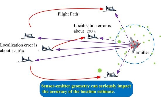
In localization estimation systems, it is well known that the sensor-emitter geometry can seriously impact the accuracy of the location estimate. In this paper, time-difference-of-arrival (TDOA) localization is applied to locate the emitter using unmanned aerial vehicle (UAV) swarms equipped with TDOA-based sensors. Different from existing studies where the variance of measurement noises is assumed to be independent and changeless, we consider a more realistic model where the variance is sensor-emitter distance-dependent. First, the measurements model and variance model based on signal-to-noise ratio (SNR) are considered. Then the Cramer–Rao low bound (CRLB) is calculated and the optimal configuration is analyzed via the distance rule and angle rule. The sensor management problem of optimizing UAVs trajectories is studied by generating a sequence of waypoints based on CRLB. Simulation results show that path optimization enhances the localization accuracy and stability.

1. Introduction

Passive localization of an emitter from its radio frequency (RF) transmissions has many applications such as search and rescue, electronic surveillance, cognitive radio networks, and wireless sensor networks. The receiving platform can employ sensors measuring angle of arrival (AOA) [1], time difference of arrival (TDOA) [2], and received signal strength (RSS) [3]. TDOA measurements construct a time difference observation equation by measuring the time difference of the emitter signal arriving at different sensors. Therefore, each time difference, corresponding to one hyperboloid, and the emitter can be obtained from two or more hyperbolas. With its high accuracy and simplicity, the TDOA localization technique is widely applied [4].

The equations of the TDOA technique are quadratic and the goal is to find the position of an emitter by solving a set of nonlinear equations obtained from TDOA measurements. The TDOA measurements can be calculated by a simple closed form, e.g., spherical intersection (SX) and spherical interpolation (SI) [5], which usually uses nonlinear least-square solutions. Furthermore, the maximum likelihood method, like the Chan algorithm, was also proposed in [6] and semidefinite programming (SDP) methods in [7]. It is well known that location accuracy depends not only on the localization algorithm but also on the sensor-emitter geometry. Therefore, the selection of an optimal configuration can further improve the location accuracy. Yang et al. [8] initially performed a theoretical analysis of the sensor-emitter geometry based on CRLB with uncorrelated TDOA measurements. Lui [9] discussed optimal sensor deployment considering the correlated TDOA measurement, which makes the configuration rule more applicable. Meng et al. [10,11] formulated an optimal configuration in centralized and decentralized types of TDOA localization and further research focused on the heterogeneous sensor network. Francisco et al. [4] applied a multi-objective optimization in sensor placement. Kim et al. [12] studied the optimal configuration of sensors with the assumption that the emitter was located far from the sensors, while the sensors were relatively close to each other. In recent years, more realistic distance-dependent noise for TOA and AOA measurements was also considered [4,13,14]. In this paper, the CRLB in TDOA localization with distance-dependent noise is calculated in both static and movable scenarios; the distance rule and angle rule of the optimal configuration are extracted, which can provide guidance in optimal sensor-emitter geometries.

The application of unmanned aerial vehicle (UAV) swarms can provide unique platforms for TDOA localization. Their characteristics of flexible movement and cooperation enable them to rapidly change current geometries to achieve higher location accuracy [15,16]. Therefore, the sensor management of real-time UAV path optimization has been a heated research issue in recent years [17]. Frew [18] presented the signal strength measurement to control the UAVs movement. Soltanizadeh et al. applied the determinant of Fisher information matrix (FIM) as the control objective function in RSS localization. Wang [19] investigated UAV path planning for tracking a target using bearing-only sensors. Alomari et al. [20] provided a path planning algorithm based on the dynamic fuzzy-logic method for a movable anchor node. Kaune [21,22] preliminarily considered the path optimization method when there was only one sensor moving platform during TDOA localization. In this paper, UAVs’ trajectories are optimized by generating a sequence of waypoints based on CRLB. The CRLB of TDOA location is not only taken as a performance estimator but also as the rule of UAV path optimization. The emitter position is solved by combining the SDP methods and an extended Kalman filter (EKF) estimator. Meanwhile, the constraints of UAV swarms are considered, such as motion and communication constraints. Therefore, the real-time path planning of UAVs is converted to nonlinear optimization with constraints. The interior penalty function method is adopted to convert the nonlinear optimization to simple unconstrained optimization so as to get the flight path of each UAV for the next time.

The rest of the paper is structured as follows. Section 2 introduces the TDOA measurement model and distance-dependent noise model. In Section 3, the optimal configuration is analyzed in both static and movable emitter scenarios based on the CRLB. Section 4 presents the optimal UAV path optimization method. Simulations and conclusions are given in Section 5 and Section 6, respectively.

2. Problem Formulation

2.1. Measurement Model

Consider that $M$ time-synchronized UAVs are applied to receive the emitted signals and measure the TOAs with the state vector of each UAV ${\chi }_i(k)={(x_i(k),y_i(k))}^T,i=1,2,\cdots M$. Let $x_t=(x_t,y_t)\in {ℝ}^2$ be the location of an unknown emitter. The TDOA measurement can be obtained by the difference between any two TOA measurements, eliminating the unknown time of emission. By multiplication of the TDOA measurements by the electromagnetic wave transmission speed, the measurement function in the range domain is obtained:

$$z_{ij}=r_i-r_j,i,j\in \{1,\dots ,M\}\wedge j\ne i,$$

(1)

with $r_i=\sqrt{(x_t-x_i{)}^2+(y_t-y_i{)}^2}$ being the distance between the emitter and receiver. Let $v_i$ denote the TOA estimation error, which is assumed to be Gaussian. Then the TDOA measurement equation can be expressed as

$${\widehat{z}}_{ij}=z_{ij}(x_t)+v_{ij},i,j\in \left\{1,\dots ,M\right\}\wedge i\ne j,v_{ij}\sim \mathcal{N}(0,{\sigma }_i^2+{\sigma }_j^2),$$

(2)

where ${\sigma }_i^2$ is the measurement variance of the i-th receiver of the UAV platform, the measurement noise $v_{ij}=v_i+v_j$ is composed of the noise at the two associated receivers and has the covariance ${\sigma }_i^2+{\sigma }_j^2$.

Without loss of generality, let the 1st receiver be the reference receiver and the others be auxiliary receivers. The variance matrix of measurement matrix ${\widehat{z}}_{1j}$ consisting of $M-1$ measurements can be represented as:

$${\Sigma }_{r1}=\left[\begin{array}{cccc}{\sigma }_1^2+{\sigma }_2^2& {\sigma }_1^2& \cdots & {\sigma }_1^2\\ {\sigma }_1^2& {\sigma }_1^2+{\sigma }_3^2& \cdots & {\sigma }_1^2\\ ⋮& ⋮& \ddots & ⋮\\ {\sigma }_1^2& {\sigma }_1^2& \cdots & {\sigma }_1^2+{\sigma }_M^2\end{array}\right].$$

(3)

Therefore, the measurement vector is given by

$$\widehat{z}=z(x_t)+w,w\sim \mathcal{N}(0,{\Sigma }_{r1}).$$

(4)

2.2. Measurement Variance Model with Distance-Dependent Noise

Considering the influence of signal frequency, bandwidth, response time, and SNR, the CRLB of the TOA measurement error variance ${\sigma }_i^2$ can be represented as [23]:

$${\sigma }_i^2=\frac{c}{\tau \cdot SN{R}_i\cdot F(f_0,B)},$$

(5)

where, $\tau$ is the observation time, $f_0$ is the center frequency, $B$ is the bandwidth of the received signal, and $c$ is some constant. High accuracy can be achieved by utilizing high-precision time of arrival measurement techniques at reasonable SNR levels. With constant emitter power and constant frequency, the variance of time-delay measurement is inversely proportional to the SNR, and the SNR is inversely proportional to $r^2$. Therefore, the relationship of the i-th receiver error and distance can be expressed as [24]:

$${\sigma }_i^2(r)=\{\begin{array}{ll}\frac{a}{SN{R}_0}\cdot \frac{r_i^2}{r_0^2}& r_i>r_0\\ \frac{a}{SN{R}_0}& r_i\le r_0\end{array},$$

(6)

where $r_0$ is the lower bound of the distance corresponding to the minimum of TOA error variance and $SN{R}_0$ is the corresponding optimal SNR at the shortest distance.

The parameter-dependent standard deviation is more complex compared with the constant deviation, so the CRLB and field of view is changing in TDOA localization. Hence, the parameter-dependent standard deviation must be taken into account for accuracy analysis.

The problem of emitter localization is to estimate the location more precisely. In this paper, we mainly study the optimal sensor configuration, which can provide two basic rules to understand the rules to improve the localization performance. Then the online sensor management problem of optimal UAVs trajectories is explored.

3. Optimal Configuration Analysis

In this section, a theoretical analysis of optimal sensor-emitter geometry in TDOA localization is given without considering any constraints. Analytic solutions are derived in both the static and movable emitter scenarios.

3.1. Static Emitter Scenario

The relative sensor-emitter geometry is closely related to the location accuracy, which can be reflected by CRLB, and the configuration corresponding to the minimum CRLB is the optimal configuration.

For unbiased estimator $\widehat{x}$ of $x$, its Cramer–Rao bound can be expressed as:

$$E\left[(x-\widehat{x}){(x-\widehat{x})}^T\right]\ge J^{-1}\triangleq CRLB\left(x\right),$$

(7)

where $J$ is the Fisher information matrix (FIM).

Then the FIM for TDOA localization with distance-dependent noise is given by [25]

$$J_{i,j}={\rm E}\left[\frac{\partial }{\partial x_i}\ln (f_{\widehat{z}}(\widehat{z};x))\frac{\partial }{\partial x_j}\ln (f_{\widehat{z}}(\widehat{z};x))\right],$$

(8)

where $i,j\in \left\{1,2\right\}$. This FIM can be divided into two parts; as for the first part,

$$J_{1,(i,j)}=\frac{\partial z(\mathrm{x})}{\partial x_i}{\Sigma }_{r1}{}^{-1}(\mathrm{x}){\left(\frac{\partial z(\mathrm{x})}{\partial x_j}\right)}^T.$$

(9)

The Jacobian matrix of the measurement set with receiver 1 as the reference receiver is

$$\begin{array}{l}\frac{\partial z(\mathrm{x})}{\partial x_1}={\left[\frac{\partial z_{12}(\mathrm{x})}{\partial x_1},\frac{\partial z_{13}(\mathrm{x})}{\partial x_1},\cdots ,\frac{\partial z_{1M}(\mathrm{x})}{\partial x_1}\right]}^T\\ ={\left[\cos ({\theta }_2)-\cos ({\theta }_1),\cos ({\theta }_3)-\cos ({\theta }_1),\cdots ,\cos ({\theta }_M)-\cos ({\theta }_1)\right]}^T\end{array}$$

(10)

$$\frac{\partial z(\mathrm{x})}{\partial x_2}={\left[\sin ({\theta }_2)-\sin ({\theta }_1),\sin ({\theta }_3)-\sin ({\theta }_1),\cdots ,\sin ({\theta }_M)-\sin ({\theta }_1)\right]}^T,$$

(11)

with ${\theta }_i$ is the angle of arrival measurement of the i-th sensor and the emitter.

For the second part, when $r_i>r_0$,

$$J_{2,(i,j)}=\frac{1}{2}Tr\left({\Sigma }_{r1}{}^{-1}(x)\frac{\partial {\Sigma }_{r1}(x)}{\partial x_i}{\Sigma }_{r1}{}^{-1}(x)\frac{\partial {\Sigma }_{r1}(x)}{\partial x_j}\right),$$

(12)

where the Jacobian matrix for computing the distance dependent FIM is expressed by

$$\frac{\partial {\Sigma }_{r1}(x)}{\partial x_1}=2\beta \left[\begin{array}{cccc}{r}_1\cos {\theta }_1+r_2\cos {\theta }_2& r_1\cos {\theta }_1& \cdots & r_1\cos {\theta }_1\\ r_1\cos {\theta }_1& r_1\cos {\theta }_1+r_3\cos {\theta }_3& \cdots & r_1\cos {\theta }_1\\ ⋮& ⋮& \ddots & ⋮\\ r_1\cos {\theta }_1& r_1\cos {\theta }_1& \cdots & r_1\cos {\theta }_1+r_{(M-1)}\cos {\theta }_{(M-1)}\end{array}\right]$$

(13)

$$\frac{\partial {\Sigma }_{r1}(x)}{\partial x_2}=2\beta \left[\begin{array}{cccc}{r}_1\sin {\theta }_1+r_2\sin {\theta }_2& r_1\sin {\theta }_1& \cdots & r_1\sin {\theta }_1\\ r_1\sin {\theta }_1& r_1\sin {\theta }_1+r_3\sin {\theta }_3& \cdots & r_1\sin {\theta }_1\\ ⋮& ⋮& \ddots & ⋮\\ r_1\sin {\theta }_1& r_1\sin {\theta }_1& \cdots & r_1\sin {\theta }_1+r_{(M-1)}\sin {\theta }_{(M-1)}\end{array}\right],$$

(14)

where $\beta =\frac{a}{SN{R}_0{r}_0^2}$.

Based on the characteristics of the FIM, the optimal configuration is analyzed via distance rule and angle rule.

(1) Distance rule

As pointed out in [26], arbitrarily selecting a reference sensor does not change the CRLB for TDOA-based source localization with distance-independent noises. Here, we extend it to the distance-dependent noise model.

Theorem 1.

Given the positions of the receivers and emitter, i.e., given distance $r_i$ and angle ${\theta }_i$ the election of reference receiver has no impact on the CRLB with distance-dependent noise.

Proof. 

Without loss of generality, receivers 1 and 2 are taken as the reference receivers. Then the TDOA measurement with different reference receivers can be represented by

$${\widehat{z}}_{r1}={\left[\begin{array}{cccc}{\widehat{z}}_{21}& {\widehat{z}}_{31}& \cdots & {\widehat{z}}_{M1}\end{array}\right]}^T=T_1{\left[\begin{array}{cccc}{\widehat{z}}_1& {\widehat{z}}_2& \cdots & {\widehat{z}}_M\end{array}\right]}^T$$

(15)

$${\widehat{z}}_{r2}={\left[\begin{array}{cccc}{\widehat{z}}_{12}& {\widehat{z}}_{32}& \cdots & {\widehat{z}}_{M2}\end{array}\right]}^T=T_2{\left[\begin{array}{cccc}{\widehat{z}}_1& {\widehat{z}}_2& \cdots & {\widehat{z}}_M\end{array}\right]}^T,$$

(16)

where $T_1$ and $T_2$ are transformation matrices and are all of dimension $\left(M-1\right)\times M$. $T_1$ and $T_2$ can be represented by

$$T_1=\left[\begin{array}{ccccc}-1& 1& 0& \cdots & 0\\ -1& 0& \ddots & \ddots & ⋮\\ ⋮& ⋮& \ddots & \ddots & 0\\ -1& 0& \cdots & 0& 1\end{array}\right]T_2=\left[\begin{array}{ccccc}1& -1& 0& \cdots & 0\\ 0& -1& 1& 0& ⋮\\ ⋮& ⋮& 0& \ddots & 0\\ 0& -1& 0& 0& 1\end{array}\right].$$

It can be seen that through an element transformation matrix, $T_2$ can be transformed to $T_1$, i.e.,

$$T_2=U_{21}{T}_1,$$

(17)

where $U_{21}$ is a $\left(M-1\right)\times \left(M-1\right)$ elementary transformation matrix. It is easy to obtain

$$\frac{\partial z_{r2}(\mathrm{x})}{\partial x_i}=\frac{\partial z_{r1}(\mathrm{x})}{\partial x_i}{U}_{21}^T$$

(18)

$${\Sigma }_{r2}=U_{21}{\Sigma }_{r1}{U}_{21}^T.$$

(19)

Then $J_{{}_{1,(i,j)}}^{r2}$ can be written as

$$\begin{array}{ll}{J}_{{}_{1,(i,j)}}^{r2}& =\frac{\partial z_{r2}(\mathrm{x})}{\partial x_i}{\Sigma }_{r2}{}^{-1}(\mathrm{x}){\left(\frac{\partial z_{r2}(\mathrm{x})}{\partial x_j}\right)}^T\\ & =\frac{\partial z_{r1}(\mathrm{x})}{\partial x_i}{U}_{21}^T{\left(U_{21}{\Sigma }_{r1}(\mathrm{x})U_{21}^T\right)}^{-1}{\left(\frac{\partial z_{r1}(\mathrm{x})}{\partial x_i}{U}_{21}^T\right)}^T\\ & =\frac{\partial z_{r1}(\mathrm{x})}{\partial x_i}\left(U_{21}^T{\left(U_{21}^T\right)}^{-1}\right){\Sigma }_{r1}{}^{-1}(\mathrm{x})\left({\left(U_{21}^T\right)}^{-1}{U}_{21}^T\right)\frac{\partial z_{r1}(\mathrm{x})}{\partial x_i}\\ & =\frac{\partial z_{r1}(\mathrm{x})}{\partial x_i}{\Sigma }_{r1}{}^{-1}(\mathrm{x})\frac{\partial z_{r1}(x)}{\partial x_i}\\ & =J_{{}_{1,(i,j)}}^{r1}\end{array}.$$

(20)

Similarly, we can get $J_{{}_{2,(i,j)}}^{r2}=J_{{}_{2,(i,j)}}^{r1}$. This completes the proof. □

Therefore, the selection of a reference receiver does not influence the CRLB with distance-dependent noise.

Theorem 2.

Given the angle ${\theta }_i,i=1,2,\cdots M$, the smaller the distance between receiver and the source, the less the localization error is.

Proof. 

Due to the meaning of $J$ and the fact that the receiver measurement noise becomes larger as the range increases, $J^{-1}$ increases. A similar proof can be found in [27], but is omitted here. This distance rule can guide UAVs to fly as close to the emitter as possible. □

(2) Angle rule

Assuming the distance between the emitter and each receiver is identical, i.e., $r_1=r_2=\cdots =r$, which means the receivers have equal noise variances, we get [6,9]

$$J_1=G{\Sigma }^{-1}(x)G^T,$$

(21)

with

$$G={[{\mathrm{g}}_{ij},\cdots ]}_{\{i,j\}\in {\mathcal{I}}_0}$$

(22)

$$g_{ij}=g_i-g_j$$

(23)

$$g_i=\left[\begin{array}{c}\frac{x_t-x_i}{\sqrt{{(x_t-x_i)}^2+{(y_t-y_i)}^2}}\\ \frac{y_t-y_i}{\sqrt{{(x_t-x_i)}^2+{(y_t-y_i)}^2}}\end{array}\right]=\left[\begin{array}{c}\cos ({\theta }_i)\\ \sin ({\theta }_i)\end{array}\right].$$

(24)

Take 1st receiver as the reference receiver and ${\mathcal{I}}_0=[\{21\},\{31\},\cdots ,\{M1\}]$ is as corresponding subset of sensor pairs, then we get

$$G=[{\mathrm{g}}_{21},{\mathrm{g}}_{31},\cdots ,{\mathrm{g}}_{M1}]$$

(25)

$${\Sigma }_{r1}(x)=2\frac{a}{SN{R}_0}\cdot \frac{r^2}{r_0^2}\left[\begin{array}{cccc}1& 1/2& \cdots & 1/2\\ 1/2& \ddots & \ddots & ⋮\\ ⋮& \ddots & \ddots & 1/2\\ 1/2& \cdots & 1/2& 1\end{array}\right].$$

(26)

Substitute it into Equation (23), with $J_1$ given by

$$J_1=\frac{r^2}{\beta }[\begin{array}{c}{\displaystyle \sum _{i=1}^M{\cos }^2({\theta }_i)}-\frac{1}{M}{\left({\displaystyle \sum _{i=1}^M\cos ({\theta }_i)}\right)}^2\\ {\displaystyle \sum _{i=1}^M\cos ({\theta }_i)\sin ({\theta }_i)}-\frac{1}{M}{\displaystyle \sum _{i=1}^M\cos ({\theta }_i)}{\displaystyle \sum _{i=1}^M\sin ({\theta }_i)}\end{array}\begin{array}{c}{\displaystyle \sum _{i=1}^M\cos ({\theta }_i)\sin ({\theta }_i)}-\frac{1}{M}{\displaystyle \sum _{i=1}^M\cos ({\theta }_i)}{\displaystyle \sum _{i=1}^M\sin ({\theta }_i)}\\ {\displaystyle \sum _{i=1}^M{\sin }^2({\theta }_i)}-\frac{1}{M}{\left({\displaystyle \sum _{i=1}^M\sin ({\theta }_i)}\right)}^2\end{array}].$$

(27)

For the second part, after the algebraic simplification in Equation (12), $J_2$ can be simplified as

$$J_2=[\begin{array}{c}\frac{2{(M-1)}^2-4}{M^2}{\displaystyle \sum _{i=1}^M{\cos }^2({\theta }_i)}+\frac{4}{M^2}{\displaystyle \sum _{i=1}^M{\displaystyle \sum _{j=1}^M\cos ({\theta }_i)}}\cos ({\theta }_j)\\ \frac{{(M-1)}^2}{M^2}{\displaystyle \sum _{i=1}^M\sin (2{\theta }_i)}+\frac{2}{M^2}{\displaystyle \sum _{i=1}^M{\displaystyle \sum _{j>i}^M\sin ({\theta }_i+{\theta }_j)}}\end{array}\begin{array}{c}\frac{{(M-1)}^2}{M^2}{\displaystyle \sum _{i=1}^M\sin (2{\theta }_i)}+\frac{2}{M^2}{\displaystyle \sum _{i=1}^M{\displaystyle \sum _{j>i}^M\sin ({\theta }_i+{\theta }_j)}}\\ \frac{2{(M-1)}^2-4}{M^2}{\displaystyle \sum _{i=1}^M{\sin }^2({\theta }_i)}+\frac{4}{M^2}{\displaystyle \sum _{i=1}^M{\displaystyle \sum _{j=1}^M\sin ({\theta }_i)}}\sin ({\theta }_j)\end{array}].$$

(28)

Combine $J_1$ and $J_2$, the FIM can be expressed as

$$J=[\begin{array}{c}{\eta }_1{\displaystyle \sum _{i=1}^M{\cos }^2({\theta }_i)}-{\eta }_2{\left({\displaystyle \sum _{i=1}^M\cos ({\theta }_i)}\right)}^2\\ {\eta }_1{\displaystyle \sum _{i=1}^M\cos ({\theta }_i)\sin ({\theta }_i)}-{\eta }_2{\displaystyle \sum _{i=1}^M\cos ({\theta }_i)}{\displaystyle \sum _{i=1}^M\sin ({\theta }_i)}\end{array}\begin{array}{c}{\eta }_1{\displaystyle \sum _{i=1}^M\cos ({\theta }_i)\sin ({\theta }_i)}-{\eta }_2{\displaystyle \sum _{i=1}^M\cos ({\theta }_i)}{\displaystyle \sum _{i=1}^M\sin ({\theta }_i)}\\ {\eta }_1{\displaystyle \sum _{i=1}^M{\sin }^2({\theta }_i)}-{\eta }_2{\left({\displaystyle \sum _{i=1}^M\sin ({\theta }_i)}\right)}^2\end{array}],$$

(29)

where ${\eta }_1=\left(\frac{2{(M-1)}^2-2}{M^2}+\frac{r^2}{\beta }\right)$, ${\eta }_2=\left(\frac{r^2}{M\beta }-\frac{2}{M^2}\right)$.

Theorem 3.

Given the ranges$r_i=r_j,\forall i,j\in \left\{1,2,\cdots N\right\}$from each receiver to the emitter, we have

$$Tr(J^{-1})\ge \frac{{\eta }_1}{4};$$

(30)

the equality holds if and only if

$$\begin{array}{l}{\displaystyle \sum _{i=1}^M\cos ({\theta }_i)=0,{\displaystyle \sum _{i=1}^M\sin ({\theta }_i)=0}}\\ {\displaystyle \sum _{i=1}^M\cos (2{\theta }_i)=0,{\displaystyle \sum _{i=1}^M\sin (2{\theta }_i)=0}}\end{array}.$$

(31)

Proof. 

Let ${\lambda }_i,i=1,2$ be the eigenvalues of $J$, which is a positive definite. Then the eigenvalues of $J^{-1}$ are $1/{\lambda }_i$, It is obvious that

$$2\le \sqrt{\left(1/{\lambda }_1+1/{\lambda }_2\right)\left({\lambda }_1+{\lambda }_2\right)}={\left(Tr(J)Tr(J^{-1})\right)}^{1/2},$$

(32)

implying that

$$Tr(J^{-1})\ge 4/Tr(J).$$

(33)

The equality holds if and only if ${\lambda }_1={\lambda }_2=\lambda$. Since $J$ is a two-dimensional symmetric positive definite matrix, according to the Courant–Fischer–Weyl principle, the equation holds when $J$ is diagonal and has equal eigenvalues. Hence it implies that

$$J=\lambda I.$$

(34)

As for the $Tr\left(J\right)$, we can obtain

$$Tr\left(J\right)={\eta }_1-{\eta }_2\left[{\left({\displaystyle \sum _{i=1}^M\cos ({\theta }_i)}\right)}^2+{\left({\displaystyle \sum _{i=1}^M\sin ({\theta }_i)}\right)}^2\right]\le {\eta }_1.$$

(35)

Combining Equations (34) and (35), we get

$$\begin{array}{l}{\displaystyle \sum _{i=1}^M\cos ({\theta }_i)=0,{\displaystyle \sum _{i=1}^M\sin ({\theta }_i)=0}}\\ {\displaystyle \sum _{i=1}^M\cos (2{\theta }_i)=0,{\displaystyle \sum _{i=1}^M\sin (2{\theta }_i)=0}}\end{array}.$$

(36)

As is known from the formulas above, when the distance between each receiver is identical, the measurement accuracy depends on the included angle ${\theta }_i$ between each receiver and the emitter. Therefore, it can be called the angle rule for the optimal configuration. □

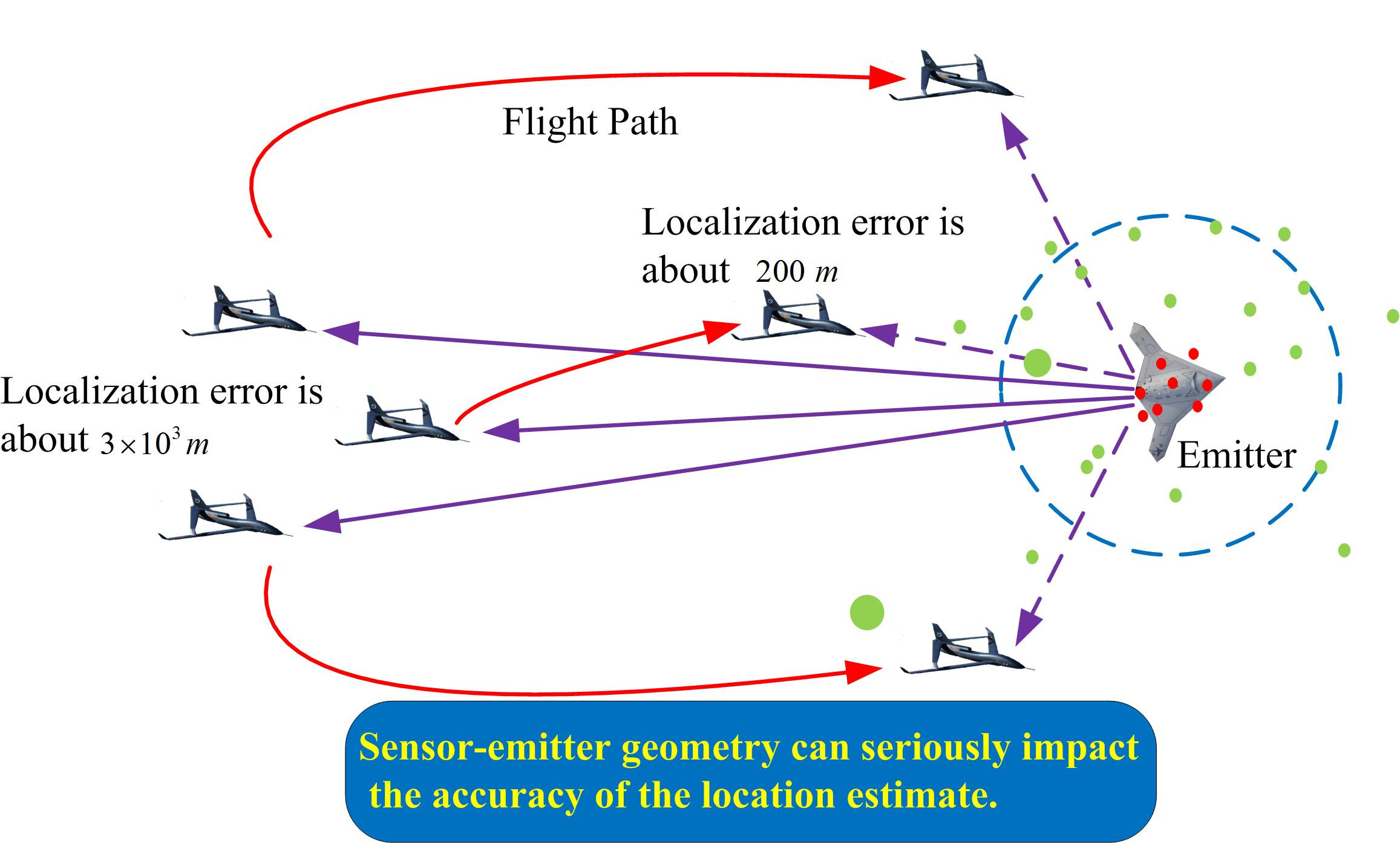
Figure 1 shows $Tr\left(J\right)$ when $M=3$ and ${\eta }_1=7$, where $A={\theta }_2-{\theta }_1$, $B={\theta }_3-{\theta }_1$ and $A+B\le 2\pi$. At this time, when $A=2\pi /3$ and $B=2\pi /3$, $Tr\left(J\right)$ has the only maximum value.

When $M\ge 3$, it is proven that the receiver distribution with uniform angular arrays (UAAs) can meet the above conditions [9]:

$${\theta }_i={\theta }_0+\frac{2\pi }{M}\left(i-1\right),i=1,2,\dots ,M,$$

(37)

where ${\theta }_i$ is any constant given on $\left[0,2\pi M/\left(M-1\right)\right)$. Figure 2 shows the optimal receiver geometries for $M=3$, $M=4$, and $M=5$. When $M=4,5$, UAAs distribution method is the unique solution of Equation (38). For $M\ge 6$, even though the optimal deployment is still given by partitions of appropriate angle each with UAA distribution, the UAAs distribution method is an optimal solution.

Remark 1.

The Cramer–Rao bound $J^{-1}$ under different distribution methods is a function of the receiver–emitter distance and angle. The optimal distribution method is to approach the distance lower bound $r_0$, according to the distance rule and select a good angular separation according to the angle rule.

For the case of arbitrary distances and angles, getting an analytic solution for the receiver–emitter geometry problem may be impossible. Some optimization algorithms can be applied to acquire a local solution.

3.2. Movable Emitter Scenario

Semidefinite programming methods [6] are applied in this paper to estimate the emitter location. Then the estimator value, calculated by SDP methods each time, can further improve the result estimated by the EKF estimator [28]. In actual applications, the SDP methods can provide initialization information for EKF. The process of the EKF filter is given by:

(1)

Predict:

$${\widehat{x}}_{k+1|k}=f_k({\widehat{x}}_{k|k})$$

(38)

$$P_{k+1|k}=f_k^x{P}_{k|k}{(f_k^x)}^T+f_k^w{Q}_{k|k}{(f_k^w)}^T.$$

(39)

(2)

Update:

$$K_{k+1|k}=P_{k+1|k}{[P_{k+1|k}+J_{k+1}^{-1}]}^{-1}$$

(40)

$$P_{k+1|k+1}=(I-K_{k+1|k})P_{k+1|k}$$

(41)

$${\widehat{x}}_{k+1|k+1}={\widehat{x}}_{k+1|k}+K_{k+1|k}\left[z_{k+1}-h_{k+1}({\widehat{x}}_{k+1|k})\right],$$

(42)

where the Jacobian matrix of the emitter movement model and the measurement model is:

$${f_k^x=\frac{\partial f_k(x_k,w_k)}{\partial x_k}|}_{\begin{array}{c}{x}_k={\widehat{x}}_{k|k}\\ w_k=0\end{array}},{f_k^w=\frac{\partial f_k(x_k,w_k)}{\partial w_k}|}_{\begin{array}{c}{x}_k={\widehat{x}}_{k|k}\\ w_k=0\end{array}}.$$

Here, we mainly focus on analyzing the optimal receiver–emitter geometry, which will enable optimal localization in terms of the posterior error covariance matrix $p_{k+1|k}$. In order to establish a relationship between $J^{-1}$ and the predicted value, Equation (43) can be expressed as follows [29]:

$$p_{k+1|k+1}={\left({(p_{k+1|k})}^{-1}+J_{k+1}\right)}^{-1}.$$

(43)

Define $p_{k+1|k}=\left[\begin{array}{cc}{p}_{11}& p_{12}\\ p_{12}& p_{22}\end{array}\right]$, $S={(p_{k+1|k})}^{-1}+J_{k+1}$ which is positive definite. Then $S$ is given by

$$S=\left[\begin{array}{cc}{J}_{(1,1)}+\frac{p_{22}}{p_{11}{p}_{22}-p_{12}^2}& J_{(1,2)}-\frac{p_{12}}{p_{11}{p}_{22}-p_{12}^2}\\ J_{(1,2)}-\frac{p_{12}}{p_{11}{p}_{22}-p_{12}^2}& J_{(2,2)}+\frac{p_{11}}{p_{11}{p}_{22}-p_{12}^2}\end{array}\right].$$

(44)

For the moveable emitter scenario, the objective is to minimize the mean square error (MSE), i.e., $Tr(p_{k+1|k+1})$, then the following results can be obtained.

Theorem 4.

For$M\ge 3$, we have

$$Tr(p_{k+1|k+1})\ge \frac{4}{J_{(1,1)}+J_{(2,2)}+\frac{p_{11}+p_{22}}{p_{11}{p}_{22}-p_{12}^2}}.$$

(45)

The equality holds if and only if

$$\{\begin{array}{c}{J}_{(1,1)}-J_{(2,2)}=\frac{\left(p_{11}-p_{22}\right)}{p_{11}{p}_{22}-p_{12}^2}\\ J_{(1,1)}=\frac{2p_{12}}{p_{11}{p}_{22}-p_{12}^2}.\end{array}$$

(46)

Proof. The proof is similar to that of Corollary 3 and is omitted here. □

The explicit solutions of the optimal configuration can be acquired when the ranges are identical. Given $r_i=r_j,\forall i,j\in \left\{1,\cdots ,M\right\}$, $S$ can be written as follows [10,11]:

$$S=[\begin{array}{c}{\eta }_1{\displaystyle \sum _{i=1}^M{\cos }^2({\theta }_i)}-{\eta }_2{\left({\displaystyle \sum _{i=1}^M\cos ({\theta }_i)}\right)}^2+\frac{p_{22}}{p_{11}{p}_{22}-p_{12}^2}\\ {\eta }_1{\displaystyle \sum _{i=1}^M\cos ({\theta }_i)\sin ({\theta }_i)}-{\eta }_2{\displaystyle \sum _{i=1}^M\cos ({\theta }_i)}{\displaystyle \sum _{i=1}^M\sin ({\theta }_i)}-\frac{p_{12}}{p_{11}{p}_{22}-p_{12}^2}\end{array}\begin{array}{c}{\eta }_1{\displaystyle \sum _{i=1}^M\cos ({\theta }_i)\sin ({\theta }_i)}-{\eta }_2{\displaystyle \sum _{i=1}^M\cos ({\theta }_i)}{\displaystyle \sum _{i=1}^M\sin ({\theta }_i)}-\frac{p_{12}}{p_{11}{p}_{22}-p_{12}^2}\\ {\eta }_1{\displaystyle \sum _{i=1}^M{\sin }^2({\theta }_i)}-{\eta }_2{\left({\displaystyle \sum _{i=1}^M\sin ({\theta }_i)}\right)}^2+\frac{p_{11}}{p_{11}{p}_{22}-p_{12}^2}\end{array}].$$

(47)

Then the optimal configuration can be acquired if and only if

$$\begin{array}{l}{\displaystyle \sum _{i=1}^M\cos ({\theta }_i)=0,{\displaystyle \sum _{i=1}^M\sin ({\theta }_i)=0}}\\ {\displaystyle \sum _{i=1}^M\cos (2{\theta }_i)=\frac{p_{11}-p_{22}}{{\eta }_1\left(p_{11}{p}_{22}-p_{12}^2\right)},{\displaystyle \sum _{i=1}^M\sin (2{\theta }_i)=\frac{p_{12}}{{\eta }_1\left(p_{11}{p}_{22}-p_{12}^2\right)}}.}\end{array}$$

(48)

If $\left|\frac{p_{11}-p_{22}}{{\eta }_1\left(p_{11}{p}_{22}-p_{12}^2\right)}\right|>M$, $\left|\frac{p_{12}}{{\eta }_1\left(p_{11}{p}_{22}-p_{12}^2\right)}\right|>M$, or $r_i$ is an arbitrary value, it is hard to find the explicit solution for optimal configuration. What can be done is to apply the results in Theorem 4 for the expression of the determinant of the CRLB, and then solve an optimization problem.

4. UAV Path Optimization

Section 3 provides the optimal configuration, without considering receiver constraints. However, in general, the UAV receiving platform is affected by its movement constraints and cannot achieve the conditions for optimal configuration within a short time [30]. Usually, the UAVs are far from the emitter; also, they are affected by the communication constraint and collision avoidance constraint. Therefore, it takes some time before reaching the optimal localization configuration.

The UAV path planning problem is a constrained optimization problem [31] that involves the calculation of UAVs waypoints at discrete time instants. The optimal trajectory is generated by minimizing the trace of the CRLB, which is analyzed in Section 3. The receiver measurements are assumed to be synchronized with waypoint updates. In addition, UAVs are assumed to be equipped with a Global Positioning System (GPS) and robust line-of-sight (LOS) datalinks [32].

Assuming the systematic UAV discrete dynamic model is [15,33]:

$$X_{k+1}=f(X_k,u_k),k=1,2,\cdots ,M,$$

(49)

where $X_k$ is the system status value $X_k={[{\chi }_1(k),\cdots ,{\chi }_M(k)]}^T$ at the time $k$, and $u_k$ is the control vector $u_k=[u_1(k),u_2(k),\cdots u_M(k)]$ of UAV at each moment. Without loss of generality, UAV1 is assigned as the reference node, and the proposed waypoint update equation of the UAV is:

$$x_i(k+1)=\left[\begin{array}{c}{x}_i(k)\\ y_i(k)\end{array}\right]+v_{0}T\left[\begin{array}{c}\cos u_i(k)\\ \sin u_i(k)\end{array}\right],$$

(50)

where $v_0$ is the UAV flight speed and $T$ is the time interval between waypoint updates. The UAVs path can be optimized by taking the CRLB as the optimization rule. Within each time interval, SDP methods and EKF are used to update emitter localization and tracking estimations.

Therefore, the objective function can be expressed as:

$$\{\begin{array}{l}\arg \min f(u_{k+1})=Tr(J_{k+1}^{-1}(r_i,{\theta }_i)),k\le 3\\ \arg \min f(u_{k+1})=Tr(P_{k+1|k+1}(r_i,{\theta }_i)),k>3\end{array}$$

(51)

$$s.t.\Vert u_i(k+1)-u_i(k)\Vert \le u_{\max }$$

(52)

$$g_{1ij}(u_k)=R_h-\Vert x_i(k+1)-{\widehat{x}}_t(k)\Vert \ge 0$$

(53)

$$g_{2ij}(u_k)=\Vert x_i(k+1)-{\widehat{x}}_t(k)\Vert -R_l\ge 0$$

(54)

$$g_{3ij}(u_k)=c_h-\Vert x_i(k+1)-x_j(k+1)\Vert \ge 0$$

(55)

$$g_{4ij}(u_k)=\Vert x_i(k+1)-x_j(k+1)\Vert -c_l\ge 0,$$

(56)

where Equation (52) is the turn rate constraint of the UAV. Equations (53) and (54) represent the distance constraint from the UAV to the emitter. Equations (55) and (56) are the UAV communication constraint and collision avoidance constraint, respectively.

Therefore, the path optimization can be converted to non-linear optimization [34]. This problem is solved by directly configuring the non-linear programming method (DCNLP) or sequential quadratic programming (SQP) [35]. Considering that only the inequality constraint is included in this constraint, the interior penalty function is adopted in this paper to convert this non-linear constraint to an unconstrained problem of minimization auxiliary function. A small calculation amount guarantees the real-time performance of the calculation. The calculation steps are as follows:

Step 1: Give the system status $X_k={[{\chi }_1(k),\cdots ,{\chi }_M(k)]}^T$ of each UAV at the time $k$, TDOA measurement $\widehat{z}$ and Equations (52)–(56).

Step 2: Use the SDP methods to calculate the emitter location value ${\widehat{x}}_t(k)$ and the estimated value $x_t(k|k)$ by using EKF estimator.

Step 3: The feasible region of non-linear Equations (53)–(56) in the constraints can be defined as:

$$S=\left\{u_k|g_{1ij}(u_k)\ge 0,g_{2ij}(u_k)\ge 0,g_{3ij}(u_k)\ge 0,g_{4ij}(u_k)\ge 0\right\}.$$

(57)

The logarithmic barrier function can be obtained as:

$$G(u_k,\gamma )=f(u_k)+\gamma B(u_k),\gamma >0,$$

(58)

where $\gamma$ is a logarithmic barrier function, $\gamma \to 0$,

$$B(u_k)=-{\displaystyle \sum _{i=1}^M\ln (g_{1ij}(u_k))}-{\displaystyle \sum _{i=1}^M\ln (g_{2ij}(u_k))}-{\displaystyle \sum _{i=1}^{M-1}{\displaystyle \sum _{j=i+1}^M\ln (g_{3ij}(u_k))}}-{\displaystyle \sum _{i=1}^{M-1}{\displaystyle \sum _{j=i+1}^M\ln (g_{4ij}(u_k))}}.$$

(59)

Therefore, the non-linear constraint is converted to an unconstrained problem. The minimum value of $G\left(u_k,\gamma \right)$ can be solved by setting the initial internal point.

Step 4: As for linear Equation (52), for the convenience of calculation, the $u_k$ solved in Step 3 can be substituted into the constrained inequality. When the constraint conditions are satisfied, it is the final output result; otherwise, the boundary value $u_{\max }$ is selected.

Step 5: The control amount $u_k$ of the UAV for the next waypoint.

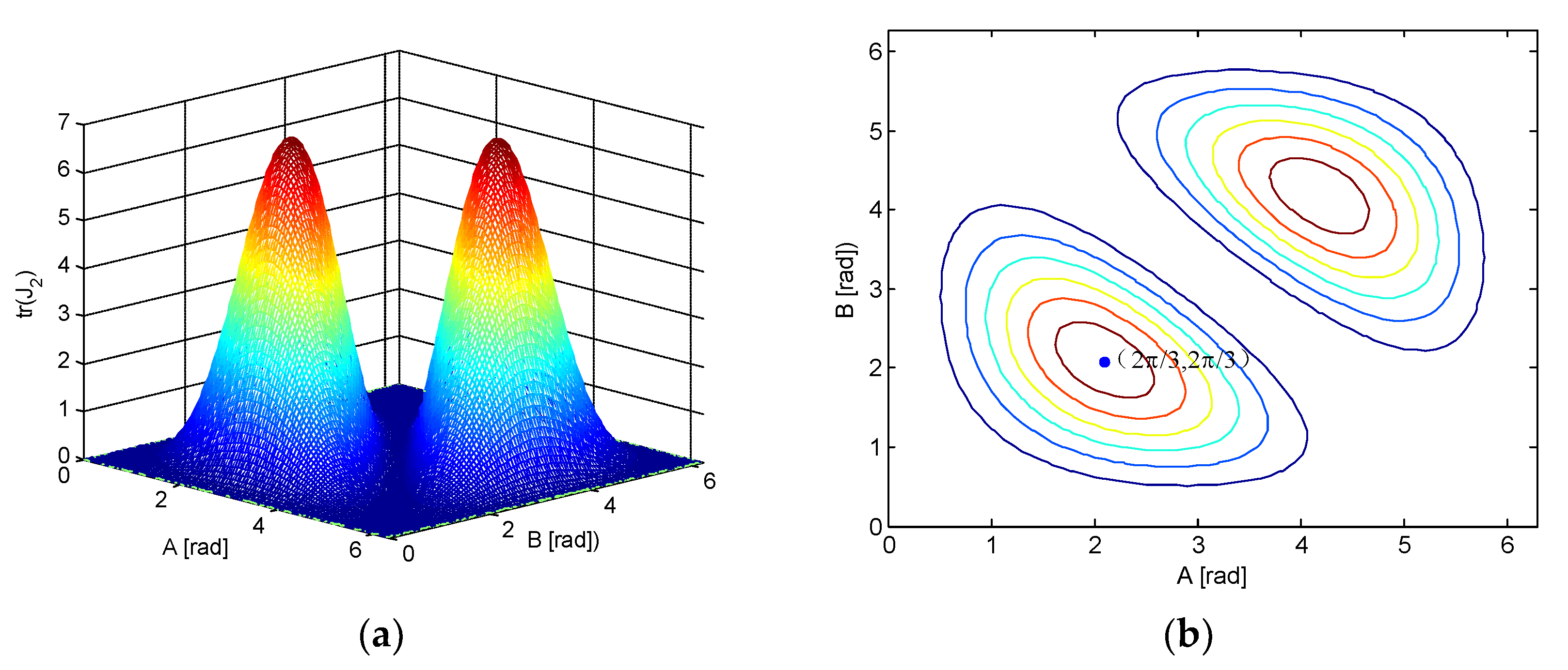
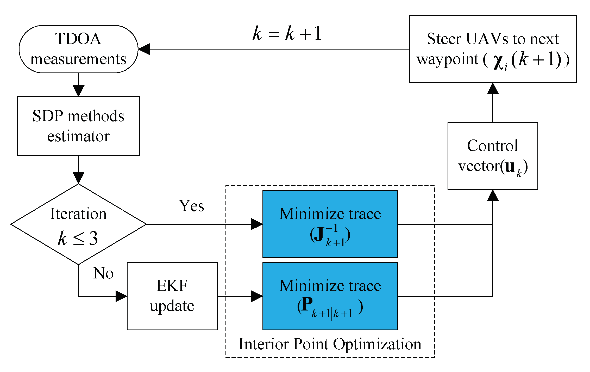
Figure 3 demonstrates the steps of the algorithm for UAV path planning based on CRLB. In this figure, $u_k$ is the output of the algorithm at time step $k$. When UAVs arrive at new waypoints, new measurements are collected and new estimations are acquired.

5. Simulation Results

In this section, four UAVs are considered to locate the static and movable emitter to verify the sensor-emitter geometries, respectively. MATLAB simulations are implemented with a 2.7 GHz Intel core processor with 8 GB of memory. The initial UAVs state vectors are ${\chi }_1(1)={\left[-9600,-5000\right]}^T$, ${\chi }_2(1)={\left[-10000,-5000\right]}^T$, ${\chi }_3(1)={\left[-10000,-5400\right]}^T$ and ${\chi }_4(1)={\left[-9600,-5400\right]}^T$. The headings for UAVs are all equal to $\pi /2$(north) at the initial moment and other key parameters are listed in

Table 1. Parameters used in simulations.

Parameters	Symbols	Values
Initial emitter position	$x_t$	${[0,0]}^T$
Fixed flight velocity	$v_0$	$150\mathrm{m}/\mathrm{s}$
Sampling time interval	$T$	$1\mathrm{s}$
Signal to noise ratio	$SN{R}_0$	$30\mathrm{dB}$
Control vector	$u_{\max }$	$15°$
Maximum distance from the UAV platform to the emitter	$R_h$	$30\mathrm{km}$
Minimum distance from the UAV platform to the emitter	$R_l$	$1000\mathrm{m}$
Safe distance between the UAV platform	$c_l$	$200\mathrm{m}$
Communication maximum distance	$c_h$	$15\mathrm{km}$
Barrier parameter for interior point optimization	$\gamma$	${10}^{-8}$

.

5.1. Angle Rule

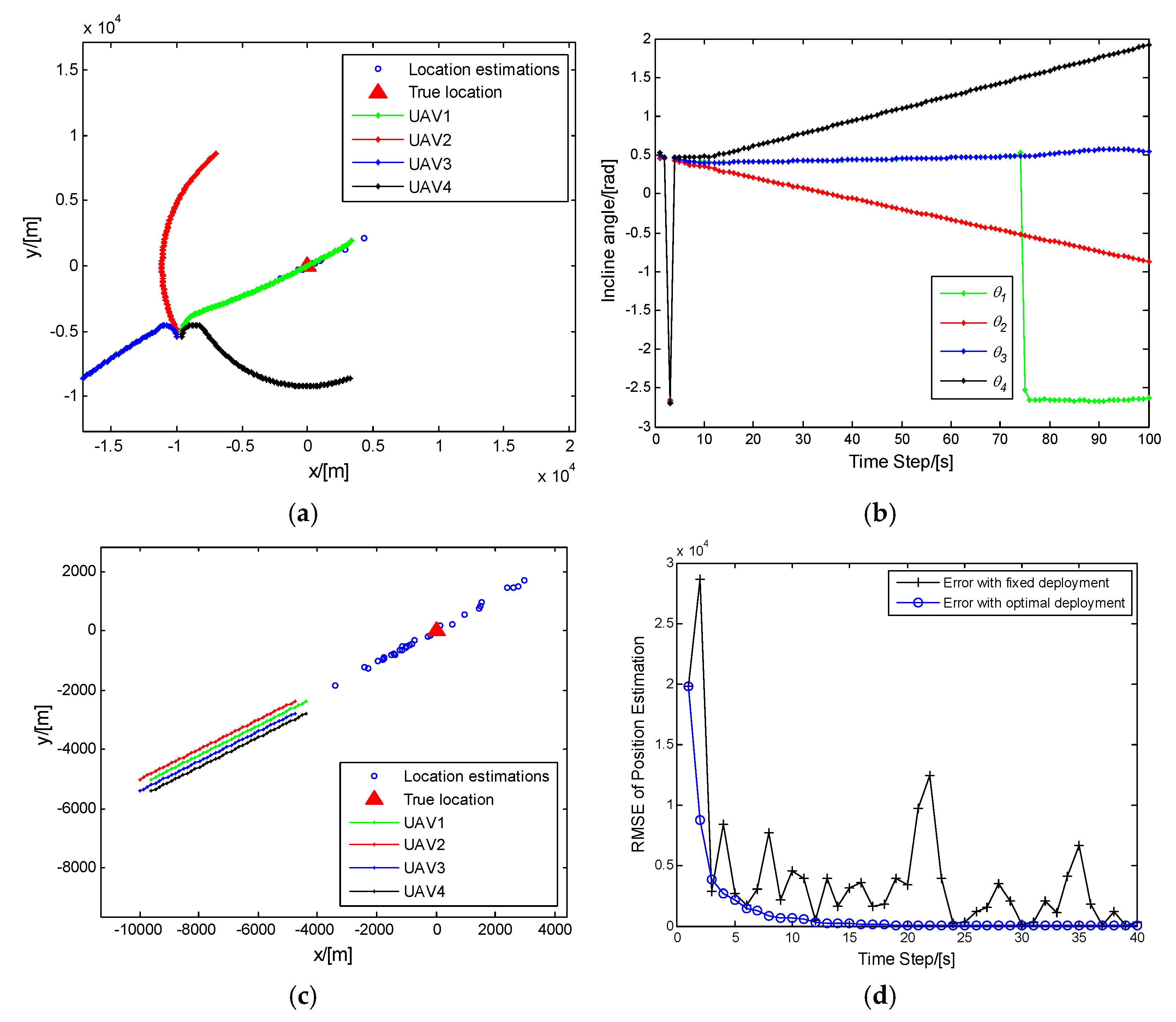
Firstly, the UAVs path optimization with only a turn rate constraint is investigated to verify the angle rule. The true emitter location is $x_t={\left[0,0\right]}^T$. Here we assume that ${\sigma }_i^2$ is irrelevant to distance $r_i$. Figure 4a,c show the optimal UAV path, taking CRLB as the rule and the straight-line UAV trajectories, respectively. The red triangle in the figure denotes the true emitter location; the small blue circles denote the estimated value of the emitter position with SDP methods and EKF estimator within each time step.

From Figure 4a,b, it can be seen that the UAVs try to fly away from each other and obtain the evolution of angle ${\theta }_i$. Meanwhile, it is noted that each UAV does not obtain effective emitter information due to the initial deployment, and the localization errors is high. After the 10th time step, the localization error drops sharply with changes in the ${\theta }_i$, emitter, as is shown in Figure 4d. Figure 4c shows the straight-line UAV trajectories, whereby each UAV is steered directly towards the estimated emitter position.

To demonstrate the effectiveness of the proposed path planning algorithm, Figure 4d shows the RMSE of optimal trajectories compared with straight-line trajectories after 50 Monte Carlo simulations. This shows that the application of the angle rule is capable of reducing the location error, while the location error with straight-line trajectories is large and apparently uncertain. However, even after all constraints are considered, it can be seen that minimizing the localization could result in baseline expansion. UAVs fly away from each other only within the constrained scope, which is not desirable in actual situations. Hence, it is impractical to reach the optimal location by relying only on the angle rule.

5.2. Combination of Angle Rule and Distance Rule

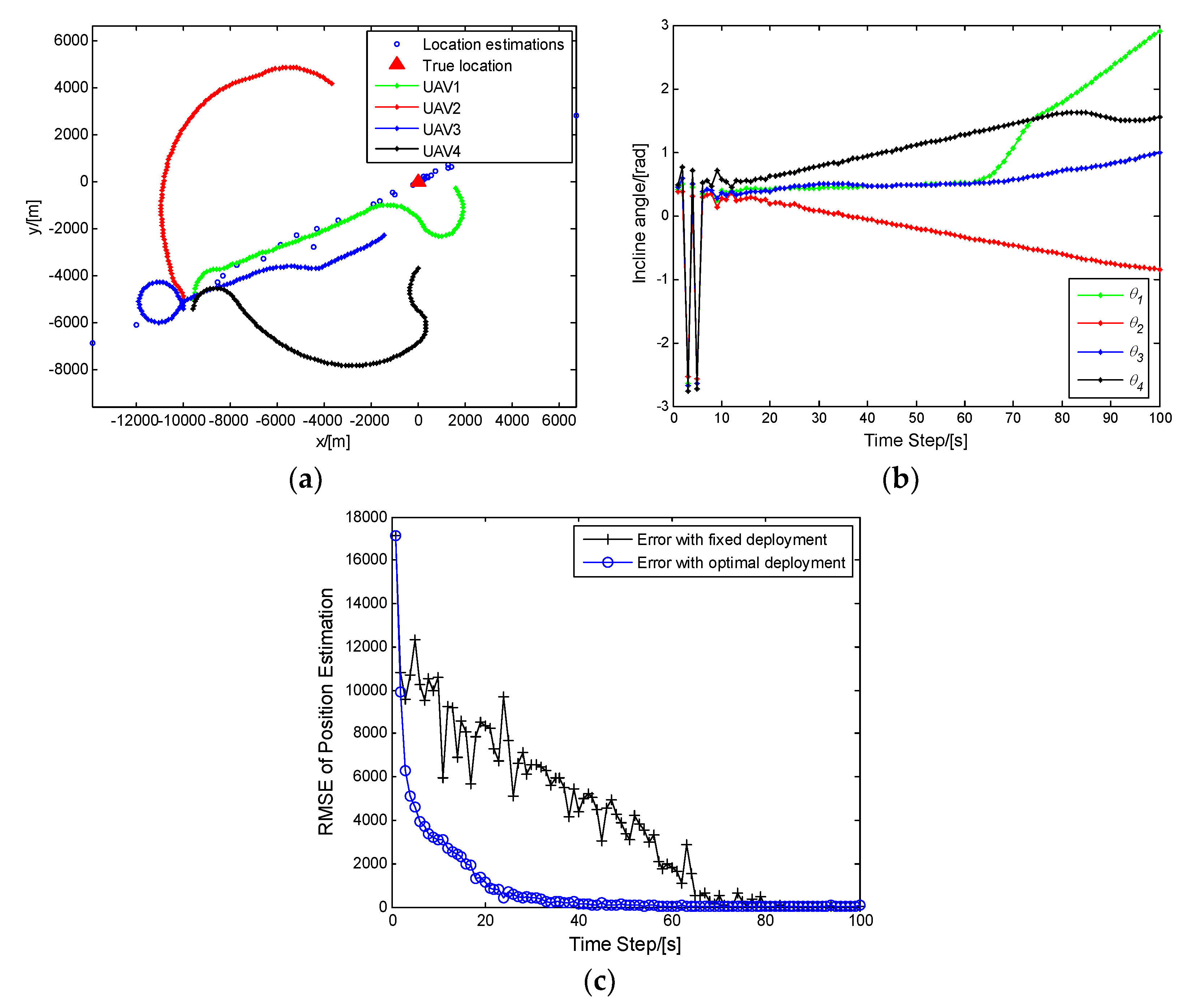
The optimal paths considering the noise variance change with distance and all constraints are included in the optimization problem. The simulation results are shown in Figure 5.

According to Figure 5a,b, the distance between each UAV and the emitter in the initial stage is nearly the same in the initial time step, so it is similar to the angle rule case: Each UAV tends to expand the detection angles to have a better view of the emitter. The initial flight direction of UAV3 is basically the same as the path in Section 5.1. After about the 10th time step, UAV3 begins to make a turn and fly toward the emitter, which is mainly caused by the distance rule. The flight path of UAV2 and UAV4 is mainly affected by the angle rule during the first several steps and they fly away from the UAV1. When large angles are obtained, they start to be affected by the distance rule and fly towards the emitter so that a balance between the angle rule and distance rule is eventually reached. UAV1 flies towards the emitter and starts to rotate around the emitter since it is affected by a lower limit $R_l$ of distance at about $t=63s$. Figure 5c shows a comparison of the optimal UAV paths and straight-line paths. The RMSE of UAVs flying with straight-line trajectories generally tends to decrease, mainly because of the distance rule. However, its location accuracy is still unstable as the relative deployment of UAVs and the emitter at certain moments are rather inappropriate for the emitter localization. Similar to the angle rule case, the localization performance using path optimization is much better than the straight-line paths. If there is a requirement to the lower RMSE, UAVs will rotate around the estimated emitter location in a fixed distance according to the angle rule.

5.3. Effect of the Number of UAVs on TDOA Localization Performance

The purpose of this simulation is to compare the localization performance with different numbers of UAVs (i.e., M = 3, 4, 5).

Figure 6 shows the evolution of RMSE corresponding to varying values of M. As can be expected, as M becomes larger, a lower and more stable RMSE is obtained.

We also notice that the objective function has a growing number of local parameters causing sensitivities to initialization with M increases. This may lead to suboptimal solutions if not initialized properly. Hence, the initialization of the target plays an important role in SDP methods. The results in Section 3 can be helpful for a proper choice of the initial measurements.

5.4. Dynamic Emitter

As for dynamic emitter, it is assumed that the emitter is uniform linear motion and the dynamic behavior of the state is described by:

$$x_t(k)=F{x}_t(k-1)+v(k).$$

(60)

The initial state is $x_t(1)={\left[0,50/\sqrt{2},0,50/\sqrt{2}\right]}^T$, with the state transition matrix given by:

$$F=\left[\begin{array}{cccc}1& \Delta T& 0& 0\\ 0& 1& 0& 0\\ 0& 0& 1& \Delta T\\ 0& 0& 0& 1\end{array}\right],$$

(61)

where $\Delta T=1s$. In order to simplify the calculation, it is assumed that the emitter flies at a speed of 50 m/s along the straight line and other constraints are the same as in the static emitter situation.

Figure 7a shows the results of location and tracking for a dynamic emitter. Different from static emitters, each UAV starts to fly towards the estimated emitter position after obtaining a certain angle. Since the distance between the emitter and the UAV changes significantly at each moment, the distance rule exerts more influence on the UAV path at this time as compared with the static emitter localization. According to Figure 7b, the location accuracy after path optimization is still high and stable as compared with a location with straight-line paths.

6. Conclusions

In this paper, we have provided an algorithm for UAV path planning based on TDOA localization. The receiver measurement model and distance-dependent noise were presented, and optimal geometry based on CRLB was investigated in both static and movable scenarios. A hybrid SDP method and EKF estimator were applied to locate the emitter and the online sensor management presented here was particularly useful for TDOA measurements. The knowledge of optimal sensor-emitter geometries provided useful tactical information and revealed important insights into the impact of sensor-emitter geometries on the performance of emitter localization and tracking. Simulation results showed that the UAV complied with distance and angle rules when looking for an optimal path. The optimized path was able to provide accurate and stable localization.

For future work, we will consider the long-term optimization, i.e., multi-step optimization, which may bring burdens for the reference receiver. Future work will also include obstacle avoidance in real applications, which may affect the localization accuracy.

References

- Jin, Y.; Liu, X.; Hu, Z.; Li, S. DOA estimation of moving sound sources in the context of nonuniform spatial noise using acoustic vector sensor. Multidimens. Syst. Signal Process. 2015, 26, 321–336. [Google Scholar] [CrossRef]
- Compagnoni, M.; Canclini, A.; Bestagini, P. Source localization and denoising: A perspective from the TDOA space. Multidimens. Syst. Signal Process. 2016, 1–26. [Google Scholar] [CrossRef]
- Chang, S.; Li, Y.; He, Y.; Wang, H. Target Localization in Underwater Acoustic Sensor Networks Using RSS Measurements. Appl. Sci. 2018, 8, 225. [Google Scholar] [CrossRef]
- Domingo-Perez, F.; Lazaro-Galilea, J.L.; Wieser, A. Sensor placement determination for range-difference positioning using evolutionary multi-objective optimization. Exp. Syst. Appl. 2016, 47, 95–105. [Google Scholar] [CrossRef]
- Malanowski, M. Two Methods for Target Localization in Multistatic Passive Radar. IEEE Trans. Aerosp. Electr. Syst. 2012, 48, 572–580. [Google Scholar] [CrossRef]
- Chan, Y.T.; Ho, K.C. A Simple and Efficient Estimator for Hyperbolic Location. IEEE Trans. Signal Process. 1994, 42, 1905–1915. [Google Scholar] [CrossRef]
- Zou, Y.; Liu, H.; Xie, W.; Wan, Q. Semidefinite Programming Methods for Alleviating Sensor Position Error in TDOA Localization. IEEE Access 2017, 5, 23111–23120. [Google Scholar] [CrossRef]
- Yang, B. Different Sensor Placement Strategies for TDOA Based Localization. In Proceedings of the ICASSP, Honolulu, HI, USA, 15–20 April 2007; pp. 1093–1096. [Google Scholar]
- Lui, K.W.K.; So, H.C. A Study of Two-Dimensional Sensor Placement Using Time-Difference-of-Arrival Measurements. Dig. Signal Process. 2009, 19, 650–659. [Google Scholar] [CrossRef]
- Meng, W.; Xie, L.; Xiao, W. Optimality Analysis of Sensor-Source Geometries in Heterogeneous Sensor Networks. IEEE Trans. Wirel. Commun. 2013, 12, 1958–1967. [Google Scholar] [CrossRef]
- Meng, W.; Xie, L.; Xiao, W. Optimal TDOA Sensor-Pair Placement With Uncertainty in Source Location. IEEE Trans. Veh. Technol. 2016, 65, 9260–9271. [Google Scholar] [CrossRef]
- Kim, S.-H.; Park, J.H.; Yoon, W.; Ra, W.-S. A note on sensor arrangement for long-distance target localization. Signal Process. 2017, 133, 18–31. [Google Scholar] [CrossRef]
- Fang, X.; Yan, W.; Zhang, F. Optimal Sensor Placement for Range-Based Dynamic Random Localization. IEEE Geosci. Remote Sens. Lett. 2015, 12, 2393–2397. [Google Scholar] [CrossRef]
- Herath, S.C.K.; Pathirana, P.N. Optimal Sensor Arrangements in Angle of Arrival (AoA) and Range Based Localization with Linear Sensor Arrays. Sensors 2013, 13, 12277–12294. [Google Scholar] [CrossRef] [PubMed] [Green Version]
- Sarunic, P.; Evans, R. Hierarchical Model Predictive Control of UAVs Performing Multitarget-Multisensor Tracking. IEEE Trans. Aeros. Electr. Syst. 2014, 50, 2253–2268. [Google Scholar] [CrossRef]
- Tripathi, A.; Saxena, N.; Mishra, K.K. A nature inspired hybrid optimisation algorithm for dynamic environment with real parameter encoding. Int. J. Bio-Inspir. Comput. 2017, 10, 24–32. [Google Scholar] [CrossRef]
- Dogancay, K. UAV Path Planning for Passive Emitter Localization. IEEE Trans. Aerosp. Electr. Syst. 2012, 48, 1150–1166. [Google Scholar] [CrossRef]
- Frew, E.; Dixon, C.; Argrow, B. Radio source localization by a cooperating UAV team. In Proceedings of the AIAA Infotech@Aerospace, Arlington, TX, USA, 26–29 September 2005. [Google Scholar]
- Wang, X.; Ristic, B.; Himed, B.; Moran, B. Joint Passive Sensor Scheduling for Target Tracking. In Proceedings of the 20th International Conference on Information Fusion, Xi’an, China, 10–13 July 2017; pp. 1671–1677. [Google Scholar]
- Alomari, A.; Phillips, W.; Aslam, N.; comeau, F. Dynamic Fuzzy-Logic Based Path Planning for Mobility-Assisted Localization in Wireless Sensor Networks. Sensors 2017, 17, 1904. [Google Scholar] [CrossRef] [PubMed]
- Kaune, R. Finding Sensor Trajectories for TDOA Based Localization—Preliminary Considerations. In Proceedings of the Workshop Sensor Data Fusion: Trends, Solutions, Applications, Bonn, Germany, 4–6 September 2012. [Google Scholar]
- Kaune, R.; Charlish, A. Online Optimization of Sensor Trajectories for Localization using TDOA Measurements. In Proceedings of the International Conference on Information Fusion, Istanbul, Turkey, 9–12 July 2013; pp. 484–491. [Google Scholar]
- Li, X.; Deng, Z.D.; Rauchenstein, L.T.; Carlson, T.J. Contributed Review: Source-localization algorithms and applications using time of arrival and time difference of arrival measurements. Rev. Sci. Instrum. 2016, 87, 041502. [Google Scholar] [CrossRef] [PubMed] [Green Version]
- Kaune, R.; Horst, J.; Koch, W. Accuracy Analysis for TDOA Localization in Sensor Networks. In Proceedings of the 14th International Conference on Information Fusion, Chicago, IL, USA, 5–8 July 2011; pp. 1647–1654. [Google Scholar]
- Huang, B.; Xie, L.; Yang, Z. TDOA-based Source Localization with Distance-dependent Noises. IEEE Trans. Wirel. Commun. 2015, 14, 468–480. [Google Scholar] [CrossRef]
- So, H.C.; Chan, Y.T.; Chan, F.K.W. Closed-form formulae for time-difference-of-arrival estimation. IEEE Trans. Signal Process. 2008, 56, 2614–2620. [Google Scholar] [CrossRef]
- Yan, W.; Fang, X.; Li, J. Formation Optimization for AUV Localization with Range-Dependent Measurements Noise. IEEE Commun. Lett. 2014, 18, 1579–1582. [Google Scholar] [CrossRef]
- Fanaei, M.; Valenti, M.C.; Schmid, N.A.; Alkhweldi, M.M. Distributed parameter estimation in wireless sensor networks using fused local observations. In Proceedings of the SPIE Defense, Security, and Sensing, Baltimore, MD, USA, 9 May 2012; p. 17. [Google Scholar]
- Bar-Shalom, Y.; Li, X.; Kirubarajan, T. Estimation with Applications to Track and Navigation; Wiley: New York, NY, USA, 2001. [Google Scholar]
- Duan, K.; Wang, Z.; Xie, W. Sparsity-based STAP algorithm with multiple measurement vectors via sparse Bayesian learning strategy for airborne radar. IET Signal Process. 2017, 11, 544–553. [Google Scholar] [CrossRef]
- Yahya, N.M.; Tokhi, M.O. A modified bats echolocation-based algorithm for solving constrained optimisation problems. Int. J. Bio-Inspir. Comput. 2017, 10, 12–23. [Google Scholar] [CrossRef]
- Nikolakopoulos, K.G.; Koukouvelas, I.; Argyropoulos, N.; Megalooikonomou, V. Quarry monitoring using GPS measurements and UAV photogrammetry. In Proceedings of the SPIE Remote Sensing, Toulouse, France, 10 October 2015; p. 8. [Google Scholar]
- Lai, Y.-C.; Ting, W.O. Design and Implementation of an Optimal Energy Control System for Fixed-Wing Unmanned Aerial Vehicles. Appl. Sci. 2016, 6, 369. [Google Scholar] [CrossRef]
- Rajput, U.; Kumari, M. Mobile robot path planning with modified ant colony optimisation. Int. J. Bio-Inspir. Comput. 2017, 9, 106–113. [Google Scholar] [CrossRef]
- Xu, D.; Xiao, R. An improved genetic clustering algorithm for the multi-depot vehicle routing problem. Int. J. Wirel. Mob. Comput. 2015, 9, 1–7. [Google Scholar] [CrossRef]
Figure 1.
3D plot of the information function for three sensors. (a) The value of ; (b) The contour plot of .
Figure 2.
Optimal receiver geometries for (a) , (b) , (c) .
Figure 3.
UAV path planning for localization based on CRLB (TDOA: time-difference-of-arrival; SDP: semidefinite programming; EKF: extended Kalman filter).
Figure 4.
(a) Optimal paths without constraints. (b) Evolution of angle changes. (c) Straight-line paths. (d) Comparison of localization performance: optimal deployment and fixed deployment.
Figure 5.
(a) Optimal paths with constraints. (b) Evolution of angle changes. (c) Comparison of localization performance: optimal deployment and fixed deployment.
Figure 6.
Evolution of RMSE with different numbers of UAVs.
Figure 7.
(a) Optimal paths for dynamic emitter location and tracking. (b) Comparison of localization performance: optimal deployment and fixed deployment.