Associative Memories to Accelerate Approximate Nearest Neighbor Search

Abstract

Nearest neighbor search is a very active field in machine learning. It appears in many application cases, including classification and object retrieval. In its naive implementation, the complexity of the search is linear in the product of the dimension and the cardinality of the collection of vectors into which the search is performed. Recently, many works have focused on reducing the dimension of vectors using quantization techniques or hashing, while providing an approximate result. In this paper, we focus instead on tackling the cardinality of the collection of vectors. Namely, we introduce a technique that partitions the collection of vectors and stores each part in its own associative memory. When a query vector is given to the system, associative memories are polled to identify which one contains the closest match. Then, an exhaustive search is conducted only on the part of vectors stored in the selected associative memory. We study the effectiveness of the system when messages to store are generated from i.i.d. uniform ±1 random variables or 0–1 sparse i.i.d. random variables. We also conduct experiments on both synthetic data and real data and show that it is possible to achieve interesting trade-offs between complexity and accuracy.

1. Introduction

Nearest neighbor search is a fundamental problem in computer science that consists of finding the data point in a previously given collection that is the closest to some query data point, according to a specific metric or similarity measure. A naive implementation of nearest neighbor search is to perform an exhaustive computation of distances between data points and the query point, resulting in a complexity linear in the product of the cardinality and the dimension of the data points.

Nearest neighbor search is found in a wide set of applications, including object retrieval, classification, computational statistics, pattern recognition, vision, data mining, and many more. In many of these domains, collections and dimensions are large, leading to unreasonable computation time when using exhaustive search. For this reason, many recent works have been focusing on approximate nearest neighbor search, where complexities can be greatly reduced at the cost of a nonzero error probability in retrieving the closest match. Most methods act either on the cardinality [1,2,3] or on the dimension [4,5,6] of the set of data points. Reducing cardinality often requires to be able to partition space in order to identify interesting regions that are likely to contain the nearest neighbor, thus reducing the number of distances to compute, whereas reducing dimensionality is often achieved through quantization techniques, and thus approximate distance computation.

In this note, we will present and investigate an alternative approach that was introduced in [7] in the context of sparse data. Its key idea is to partition the patterns into equal-sized classes and to compute the overlap of an entire class with the given query vector using associative memories based on neural networks. If this overlap of a given class is above a certain threshold, we decide that the given vector is similar to one of the vectors in the considered class, and we perform exhaustive search on this class, only. Obviously, this is a probabilistic method that comes with a certain probability of failure. We will impose two restrictions on the relation between dimension and the size of the database, or equivalently, between dimension and the number of vectors in each class: on the one hand, we want the size of the database to be so large that the algorithm is efficient compared to other methods (primarily exhaustive search), on the other hand, we need it to be small enough, to let the error probability converge to zero, as the dimension (and possibly the size of the database) converges to infinity.

More precisely, in this note, we will consider two principally different scenarios: one where the input patterns are sparse. Here, one should think of the data points as sequences of signals of a certain length, where only very rarely a signal is sent. This will be modeled by a sequences of zeroes and ones with a vast majority of zeros and another scenario. The other situation will be a scenario of “dense” patterns, where about half of the times there is a signal. We will in this case assume that the data points are “unbiased”. This situation is best modeled by choosing the coordinates of all the input vector as independent and identically distributed (i.i.d.) $\pm 1$-random variables with equal probabilities for $+1$ and for $-1$. The advantage of these models is that they are accessible to a rigorous mathematical treatment and pretty close to the more realistic situations studied in Section 5.

Even though the principal approach is similar (we have to bound the probability of an error), both cases have their individual difficulties. As a matter of fact, similar problems occur when analyzing the Hopfield model [8] of neural networks for unbiased patterns (see, e.g., [9,10,11]) or for sparse, biased patterns (see, e.g., [12,13]). On a technical level, the bounds on the error probabilities in the theoretical part of the paper (Section 3 and Section 4) are obtained by a union bound and further on by an application of an exponential Chebyshev inequality. This is one of the most general ways to obtain upper bounds on probabilities and therefore is widely used. However, in general, the challenge is always to obtain appropriate estimates for the moment generating functions in question (examples are [10,14,15]). Here, we use a Lindeberg principle that is new in this context and allows us to replace our random variables with Gaussian ones, Taylor expansion techniques for the exponents, as well as Gaussian integration to obtain the desired bounds. We will analyze the situation of sparse patterns in Section 3, while Section 4 is devoted to the investigation of the situation where the patterns are unbiased and dense. In Section 5, we will support our findings with simulations on classical approximate nearest neighbor search benchmarks. These will also reveal the interplay between the various parameters in our model and confirm the theoretical predictions of Section 3 and Section 4. The simulations on real data also give ideas for further research directions. In Section 6 we summarize our results.

2. Related Work

Part of the literature focuses on using tree-based methods to partition space [2,16,17], resulting in difficulties when facing high dimension spaces [1]. When facing real-valued vectors, many techniques proposed binary encoding of vectors [3,18,19], leading to very efficient reductions in time complexity. As a matter of fact, the search in Hamming space can be performed very efficiently, but it is well known that premature discretization of data usually leads to significant loss in precision.

Another line of work is to rely on quantization techniques based on Product Quantization (PQ) or Locality Sensitive Hashing (LSH). In PQ [4], vectors were split into subvectors. Each subvector space is quantized independently of the others. Then, a vector is quantized by concatenating the quantized versions of its subvectors. Optimized versions of PQ have been proposed by performing joint optimization [20,21]. In LSH, multiple hash functions were defined, resulting in storing each point index multiple times [5,22,23,24]. Very recently, the authors have proposed [25] to learn indexes using machine learning methods, resulting in promising performance.

In [7], the authors proposed to split data points into multiple parts, each one stored in its own sparse associative memory. The ability of these memories to store a large number of messages resulted in very efficient reduction in time complexity when data points were sparse binary vectors. In [6], the authors proposed to use the sum of vectors instead of associative memories and discussed optimization strategies (including online scenarios). The methods we analyze in this note are in the same vein.

3. Search Problems with Sparse Patterns

In this section, we will treat the situation where we try to find a pattern that is closest to some input pattern and all the patterns are binary and sparse.

To be more precise, assume that we are given nsparse vectors or patterns $x^{\mu },\mu =1,\dots ,n$ with $x^{\mu }\in {\{0,1\}}^d$ for some (large) d. Assume that the $(x^{\mu })$ are random and i.i.d. and have i.i.d. coordinates such that:

$$\mathbb{P}(x_i^{\mu }=1)=\frac{c}{d}=1-\mathbb{P}(x_i^{\mu }=0)$$

for all $i=1,\dots ,d$ and all $\mu =1,\dots ,n$. To describe a sparse situation, we will assume c depends on d, such that $c/d\to 0$ as c and d become large. We will even need this convergence to be fast enough. Moreover, we will always assume that there is an $x^{\mu }$ such that the query pattern $x^0$ has a macroscopically large overlap with $x^{\mu }$, hence that ${\sum }_{l=1}^d{x}_l^0{x}_l^{\mu }$ is of order c.

We will begin with the situation that $x^0=x^{\mu }$ for an index $\mu$. The situation where $x^0$ is a perturbed version of $x^{\mu }$ is then similar.

The algorithm proposed in [7] proposes to partition the patterns into equal-sized classes ${\mathcal{X}}^1,\dots {\mathcal{X}}^q$, with $|{\mathcal{X}}^i|=k$ for all $i=1,\dots q$. Thus, $n=kq$. Afterwards, one computes the score:

$$s({\mathcal{X}}^i,x^0)=\sum _{\mu :x^{\mu }\in {\mathcal{X}}^i}\sum _{l,m=1}^d{x}_l^0{x}_m^0{x}_l^{\mu }{x}_m^{\mu }$$

for each of these classes and takes the class ${\mathcal{X}}^i$ with the highest score. Then, on this class, one performs exhaustive search. We will analyze under which condition on the parameters this algorithm works well and when it is effective. To this end, we will show the following theorem.

Theorem 1.

Assume that the query pattern is equal to one of the patterns in the database. The algorithm described above works asymptotically correctly, i.e., with an error probability that converges to zero and is efficient, i.e., requires less computations than exhaustive search, if:

1. 

$d\ll k\ll d^2$, i.e., $\frac{k}{d^2}\to 0$ and $\frac{k}{d}\to \infty$,

2. 

$c\ll d$ and $c\ll {\left(\frac{d^7}{k^3}\right)}^{\frac{1}{6}}$

3. 

and $q{e}^{-\frac{1}{33}\frac{d^2}{k}}\to 0$.

Proof. 

To facilitate notation, assume that $x^0=x^1$ (which is of course unknown to the algorithm), that $x^1\in {\mathcal{X}}^1$ and that $x_i^1=1$ for the first $\tilde{c}$ indices i and that $x_i^1=0$ for the others. Note that for any $\epsilon >0$, with high probability (when c and d become large), we are able to assume that $\frac{\tilde{c}}{d}\in \left(\frac{c}{d}(1-\epsilon ),\frac{c}{d}(1+\epsilon )\right)$. Then, for any i, we have $s({\mathcal{X}}^i,x^0)={\sum }_{\mu :x^{\mu }\in {\mathcal{X}}^i}{\sum }_{l,m=1}^{\tilde{c}}{x}_l^{\mu }{x}_m^{\mu }$ and in particular:

$$s({\mathcal{X}}^1,x^0)={\tilde{c}}^2+\sum _{\genfrac{}{}{0pt}{}{\mu :x^{\mu }\in {\mathcal{X}}^1}{\mu \ne 1}}\sum _{l,m=1}^{\tilde{c}}{x}_l^{\mu }{x}_m^{\mu }.$$

We now want to show that for a certain range of parameters $n,k$ and d, this algorithm works reliably, i.e., we want to show that:

$$\mathbb{P}(\exists i\ge 2:s({\mathcal{X}}^i,x^0)\ge s({\mathcal{X}}^1,x^0))\to 0\mathrm{as}d\to \infty .$$

Now, since, c and $\tilde{c}$ are close together when divided by d, we will replace $\tilde{c}$ by c everywhere without changing the proof. Trivially,

$$\mathbb{P}(\exists i\ge 2:s({\mathcal{X}}^i,x^0)\ge s({\mathcal{X}}^1,x^0))\le q\mathbb{P}(s({\mathcal{X}}^2,x^0)\ge s({\mathcal{X}}^1,x^0))$$

and we just need to bound the probability on the right-hand side. Taking $X_{\mu }$ to be i.i.d. $B(c,\frac{c}{d})$-distributed random variables, we may rewrite the probability on the right-hand side as:

$$\mathbb{P}(s({\mathcal{X}}^2,x^0)\ge s({\mathcal{X}}^1,x^0))=\mathbb{P}(\sum _{\mu =1}^k{X}_{\mu }^2-\sum _{\mu =k+1}^{2k-1}{X}_{\mu }^2\ge c^2).$$

Centering the variables, we obtain:

$$\begin{array}{cc}& \mathbb{P}(\sum _{\mu =1}^k{X}_{\mu }^2-\sum _{\mu =k+1}^{2k-1}{X}_{\mu }^2\ge c^2)\hfill \\ =& \mathbb{P}(\sum _{\mu =1}^k{(X_{\mu }-\frac{c^2}{d})}^2-\sum _{\mu =k+1}^{2k-1}{(X_{\mu }-\frac{c^2}{d})}^2+2\frac{c^2}{d}(\sum _{\mu =1}^k{X}_{\mu }-\sum _{\mu =k+1}^{2k-1}{X}_{\mu })-\frac{c^4}{d^2}\ge c^2)\hfill \end{array}$$

Now, as $({\sum }_{\mu =1}^k{X}_{\mu }-{\sum }_{\mu =k+1}^{2k-1}{X}_{\mu })-\frac{c^4}{d^2}\le ({\sum }_{\mu =1}^k{X}_{\mu }-{\sum }_{\mu =k+1}^{2k-1}{X}_{\mu })$, we arrive at:

$$\begin{array}{cc}& \mathbb{P}(\sum _{\mu =1}^k{X}_{\mu }^2-\sum _{\mu =k+1}^{2k-1}{X}_{\mu }^2\ge c^2)\hfill \\ \le & \mathbb{P}(\sum _{\mu =1}^k{(X_{\mu }-\frac{c^2}{d})}^2-\sum _{\mu =k+1}^{2k-1}{(X_{\mu }-\frac{c^2}{d})}^2\ge \frac{c^2}{2})+\mathbb{P}(\sum _{\mu =1}^k{X}_{\mu }-\sum _{\mu =k+1}^{2k-1}{X}_{\mu }\ge \frac{d}{4})\hfill \end{array}$$

Let us treat the last term first. For $t>0$:

$$\begin{array}{cc}& \mathbb{P}(\sum _{\mu =1}^k{X}_{\mu }-\sum _{\mu =k+1}^{2k-1}{X}_{\mu }\ge \frac{d}{4})\le e^{-t\frac{d}{4}}{(\mathbb{E}{e}^{t{X}_1})}^k{(\mathbb{E}{e}^{-t{X}_1})}^{k-1}\hfill \\ =& e^{-t\frac{d}{4}}{\left(1+\frac{c}{d}(e^t-1)\right)}^{kc}{\left(1+\frac{c}{d}(e^{-t}-1)\right)}^{(k-1)c}\hfill \\ =& e^{-t\frac{d}{4}}{\left(1+\frac{c}{d}(t+\frac{t^2}{2}+\frac{t^3}{6}+\mathcal{O}(t^4))\right)}^{kc}{\left(1+\frac{c}{d}(-t+\frac{t^2}{2}-\frac{t^3}{6}+\mathcal{O}(t^4))\right)}^{(k-1)c}\hfill \\ \le & e^{-t\frac{d}{4}}exp\left(\frac{c^2}{d}t+k\frac{c^2}{d}{t}^2+\frac{c^2}{3d}{t}^3+\mathcal{O}(\frac{c^2}{d}k{t}^4)\right)\hfill \end{array}$$

Now, we take $t={\epsilon }_d\sqrt[4]{\frac{d}{k{c}^2}}$, which implies that:

$$\begin{array}{c}\mathbb{P}(\sum _{\mu =1}^k{X}_{\mu }-\sum _{\mu =k+1}^{2k-1}{X}_{\mu }\ge \frac{d}{4})\le exp\left(-{\epsilon }_d\sqrt[4]{\frac{d^5}{256k{c}^2}}+{\epsilon }_d\sqrt[4]{\frac{c^6}{k{d}^3}}+{\epsilon }_d^2\sqrt[4]{\frac{c^4{k}^2}{d^2}}+{\epsilon }_d^3\sqrt[4]{\frac{c^2}{81d{k}^3}}+\mathcal{O}({\epsilon }_d^4)\right)\hfill \end{array}$$

Now, $\frac{c^2}{81d{k}^3}\to 0$ due to our assumptions $c\ll d\ll k$. Moreover, $\frac{d^5}{256k{c}^2}\gg \frac{c^6}{k{d}^3}$, since $c\ll d$. Hence, we just need to consider the negative term in the exponent and ${\epsilon }_d^2\sqrt[4]{\frac{c^4{k}^2}{d^2}}$, which justifies our hypothesis $c\ll {\left(\frac{d^7}{k^3}\right)}^{\frac{1}{6}}$.

The other summand is slightly more complicated: note that $\mathbb{V}(X_{\mu }-\frac{c^2}{d})\approx \frac{c^2}{d}$; thus, we compute for $t>0$:

$$\begin{array}{cc}& \mathbb{P}(\sum _{\mu =1}^k{(X_{\mu }-\frac{c^2}{d})}^2-\sum _{\mu =k+1}^{2k-1}{(X_{\mu }-\frac{c^2}{d})}^2\ge \frac{c^2}{2})=\mathbb{P}\left(\sum _{\mu =1}^k{\left(\frac{X_{\mu }-\frac{c^2}{d}}{\sqrt{\frac{c^2}{d}}}\right)}^2-\sum _{\mu =k+1}^{2k-1}{\left(\frac{X_{\mu }-\frac{c^2}{d}}{\sqrt{\frac{c^2}{d}}}\right)}^2\ge \frac{d}{2}\right)\hfill \\ \le & e^{-t\frac{d}{2}}{\left(\mathbb{E}{e}^{t{\left(\frac{X_{\mu }-\frac{c^2}{d}}{\sqrt{\frac{c^2}{d}}}\right)}^2}\right)}^k{\left(\mathbb{E}{e}^{-t{\left(\frac{X_{\mu }-\frac{c^2}{d}}{\sqrt{\frac{c^2}{d}}}\right)}^2}\right)}^{k-1}\hfill \end{array}$$

where on the right-hand side, we can take any fixed $\mu$.

To estimate the expectations, we will apply a version of Lindeberg’s replacement trick [26,27] or in a similar spirit to the computation below [28]. To this end, assume that $S_c:=\frac{X_{\mu }-\frac{c^2}{d}}{\sqrt{\frac{c^2}{d}}}\stackrel{d}{=}{\sigma }_1+\dots +{\sigma }_c$, for appropriately centered i.i.d. Bernoulli random variables ${\sigma }_k$ with variance one. Moreover, let $\xi =\frac{1}{\sqrt{c}}{\sum }_{i=1}^c{\xi }_i$, where the $({\xi }_i)$ are i.i.d. standard Gaussian random variables. Finally, set:

$$T_k:=\frac{1}{\sqrt{c}}({\sigma }_1+\cdots +{\sigma }_{k-1}+{\xi }_{k+1}+\cdots +{\xi }_c)$$

and $f(x)=e^{t{x}^2}$. Then, we obtain by Taylor expansion:

$$\begin{array}{cc}& \left|\mathbb{E}\left(f\left(S_c\right)-f(\xi )\right)\right|\le \sum _{k=1}^c\left|\mathbb{E}\left[f\left(\frac{1}{\sqrt{c}}(T_k+{\sigma }_k)\right)-f\left(\frac{1}{\sqrt{c}}(T_k+{\xi }_k)\right)\right]\right|\hfill \\ \le & \sum _{k=1}^c\left|\mathbb{E}\left[f^{\prime }\left(\frac{T_k}{\sqrt{c}}\right)\frac{1}{\sqrt{c}}({\sigma }_k-{\xi }_k)+\frac{1}{2}{f}^{\prime \prime }\left(\frac{T_k}{\sqrt{c}}\right)\frac{1}{c}({\sigma }_k^2-{\xi }_k^2)\right]\right|+\frac{1}{6c^{3/2}}\sum _{k=1}^c\left|\mathbb{E}\left[f^{(3)}({\zeta }_1){\sigma }_k^3-\mathbb{E}{f}^{(3)}({\zeta }_2){\xi }_k^3\right]\right|,\hfill \end{array}$$

where ${\zeta }_1$ and ${\zeta }_2$ are random variables that lie within the interval $[T_k,T_k+{\sigma }_k]$ and $[T_k,T_k+{\xi }_k]$, respectively (possibly with the right and left boundary interchanged, if ${\sigma }_k$ or ${\xi }_k$ are negative). First of all, observe that for each k, the random variable $T_k$ is independent of the ${\xi }_k$ and ${\sigma }_k$, and ${\xi }_k$ and ${\sigma }_k$ have matching first and second moments. Therefore:

$$\sum _{k=1}^c\left|\mathbb{E}\left[f^{\prime }\left(\frac{T_k}{\sqrt{c}}\right)\frac{1}{\sqrt{c}}({\sigma }_k-{\xi }_k)+\frac{1}{2}{f}^{″}\left(\frac{T_k}{\sqrt{c}}\right)\frac{1}{c}({\sigma }_k^2-{\xi }_k^2)\right]\right|=0.$$

For the second term on the right-hand side, we compute:

$$f^{(3)}(x)=(12t^{2}x+8t^3{x}^3)f(x).$$

Observe that $\mathbb{E}\left[{(\xi )}^{\nu }{e}^{t{\xi }^2}\right]<\infty$ for $\nu =0,1,2,3$ for t small enough and the expectation $\mathbb{E}\left[{\left(\frac{X_{\mu }-\frac{c^2}{d}}{\sqrt{\frac{c^2}{d}}}\right)}^{\nu }f\left(\frac{X_{\mu }-\frac{c^2}{d}}{\sqrt{\frac{c^2}{d}}}\right)\right]$ is uniformly bounded in the number of summands c for $\nu =0,1,2,3$ and if t is small enough. Finally, ${\zeta }_1$ and ${\zeta }_2$ have the form $T_k+{\alpha }_k\frac{{\xi }_k}{\sqrt{c}}+{\beta }_k{\sigma }_k$ for some coefficients ${\alpha }_k$ and ${\beta }_k$ with $0\le |{\alpha }_k|,|{\beta }_k|\le 1$. Therefore, $\left|\mathbb{E}\left[f^{(3)}({\zeta }_1){\sigma }_k^3-\mathbb{E}{f}^{(3)}({\zeta }_2){\xi }_k^3\right]\right|$ is of order $t^2{e}^{t/\sqrt{c}}$, i.e., for fixed t of constant order, and:

$$\frac{1}{6c^{3/2}}\sum _{k=1}^c\left|\mathbb{E}\left[f^{(3)}({\zeta }_1){\sigma }_k^3-\mathbb{E}{f}^{(3)}({\zeta }_2){\xi }_k^3\right]\right|=\mathcal{O}(\frac{t^2{e}^{t\sqrt{c}}}{\sqrt{c}})={\mathcal{O}}_t(\frac{1}{\sqrt{c}})$$

where ${\mathcal{O}}_t$ denotes an upper bound by a constant that may depend on t. This notation (and the implied crude way to deal with the t-dependence) is justified, because from the next line on, we will just concentrate on t values that are smaller than $\frac{1}{2}$. For those, $\frac{t^2{e}^{t/\sqrt{c}}}{\sqrt{c}}\le \frac{1}{\sqrt{c}}$.

Moreover, we have for t smaller than $1/2$ by Gaussian integration:

$$\mathbb{E}\left[f(\xi )\right]=\mathbb{E}\left[e^{t{\xi }^2}\right]=\frac{1}{\sqrt{1-2t}}.$$

(1)

Therefore, writing:

$$\mathbb{E}\left[f(S_c)\right]\le \left|\mathbb{E}[f(\xi )]\right|+\left|\mathbb{E}[f(S_c)-f(\xi )]\right|,$$

We obtain:

$$\begin{array}{c}{\left(\mathbb{E}\left[e^{t\frac{X_{\mu }^2-\frac{c^2}{d}}{\sqrt{\frac{c^2}{d}}}}\right]\right)}^k\le e^{-\frac{k}{2}log(1-2t)}{\left(1+e^{\frac{1}{2}log(1-2t)}{\mathcal{O}}_t(\frac{1}{\sqrt{c}})\right)}^k.\hfill \end{array}$$

In a similar fashion, we can also bound:

$$\begin{array}{c}{\left(\mathbb{E}\left[e^{-t\frac{X_{\mu }^2-\frac{c^2}{d}}{\sqrt{\frac{c^2}{d}}}}\right]\right)}^{k-1}\le e^{-\frac{k-1}{2}log(1+2t)}{\left(1+e^{\frac{1}{2}log(1+2t)}{\mathcal{O}}_t(\frac{1}{\sqrt{c}})\right)}^{k-1},\hfill \end{array}$$

where now, we make use of $\mathbb{E}\left[e^{-t{\xi }^2}\right]=\frac{1}{\sqrt{1+2t}}$ instead of (1).

Hence, by Taylor expansion of the logarithm altogether, we obtain:

$$\begin{array}{c}{\displaystyle \mathbb{P}(\sum _{\mu =1}^k{(X_{\mu }-\frac{c^2}{d})}^2-\sum _{\mu =k+1}^{2k-1}{(X_{\mu }-\frac{c^2}{d})}^2\ge \frac{c^2}{2})\le e^{-t\frac{d}{2}}{e}^{2k{t}^2+\mathcal{O}(t+t^2\frac{k}{\sqrt{c}}+k{t}^4)}.}\hfill \end{array}$$

(2)

Note that we will always assume that $c\to \infty$ such that $\frac{k}{\sqrt{c}}$ is negligible with respect to k. Now, we choose $t=\frac{d}{8k}$. This, in particular, ensures that t converges to zero for large dimensions and therefore especially that (1) can be applied; we obtain that asymptotically:

$$\mathbb{P}(\sum _{\mu =1}^k{(X_{\mu }-\frac{c^2}{d})}^2-\sum _{\mu =k+1}^{2k-1}{(X_{\mu }-\frac{c^2}{d})}^2\ge \frac{c^2}{2})\le e^{-\frac{1}{33}\frac{d^2}{k}}.$$

(3)

Indeed, keeping the leading order term from the $\mathcal{O}$-expression in (2) with our choice of t, we obtain that asymptotically:

$$\mathbb{P}(\sum _{\mu =1}^k{(X_{\mu }-\frac{c^2}{d})}^2-\sum _{\mu =k+1}^{2k-1}{(X_{\mu }-\frac{c^2}{d})}^2\ge \frac{c^2}{2})\le e^{-\frac{1}{32}\frac{d^2}{k}+\mathcal{O}(\frac{d^4}{k^3})}=e^{-\frac{1}{32}\frac{d^2}{k}(1+\mathcal{O}(\frac{d^2}{k^2}))}.$$

As $d\ll k$, the term $(1+\mathcal{O}(\frac{d^2}{k^2}))$ will get arbitrarily close to one; hence, (3) follows. However, the right-hand side of (3) goes to zero, whenever $d^2\gg k$. Hence, for $d\ll k\ll d^2$, we obtain that the method works fine if $c\ll d$, $c\ll {\left(\frac{d^7}{k^3}\right)}^{\frac{1}{6}}$ and $q\ll e^{\frac{1}{33}\frac{d^2}{k}}$, which are our last conditions. ☐

In a very similar fashion, we can treat the case of an input pattern that is a corrupted version of one of the vectors in the database.

Corollary 1.

Assume that the input pattern $x^0$ has a macroscopic overlap with one of the patterns in the database, i.e., ${\sum }_{l=1}^d{x}_l^0{x}_l^{\mu }=\alpha c$, for a $\alpha \in (0,1)$, and $x^0$ has c entries equal to one and $d-c$ indices equal to zero. The algorithm described above works asymptotically correctly, i.e., with an error probability that converges to zero, and is efficient if:

1. 

$d\ll k\ll d^2$,

2. 

$c\ll d$ and $c\ll {\left(\frac{d^7}{k^3}\right)}^{\frac{1}{6}}$

3. 

and $q{e}^{-\frac{{\alpha }^4}{33}\frac{d^2}{k}}\to 0$.

Proof. 

The proof is basically a rerun of the proof of Theorem 1. Again, without loss of generality, assume that $x^1$ is our target pattern in the database such that ${\sum }_{l=1}^d{x}_l^0{x}_l^1=\alpha c$, that $x^1\in {\mathcal{X}}^1$ and that $x_i^0=1$ for the first c indices i and that $x_i^0=0$ for the others. Then, for any i, we have:

$$s({\mathcal{X}}^1,x^0)={\alpha }^2{c}^2+\sum _{\genfrac{}{}{0pt}{}{\mu :x^{\mu }\in {\mathcal{X}}^1}{\mu \ne 1}}\sum _{l,m=1}^c{x}_l^{\mu }{x}_m^{\mu }$$

while $s({\mathcal{X}}^i,x^0)$ is structurally the same as in the previous proof. Therefore, following the lines of the proof of Theorem 1 and using the notation introduced there, we find that:

$$\begin{array}{cc}& \mathbb{P}(\exists i\ge 2:s({\mathcal{X}}^i,x^0)\ge s({\mathcal{X}}^1,x^0))\le q(s({\mathcal{X}}^2,x^0)\ge s({\mathcal{X}}^1,x^0))\hfill \\ =& q\mathbb{P}(\sum _{\mu =1}^k{(X_{\mu }-\frac{c^2}{d})}^2-\sum _{\mu =k+1}^{2k-1}{(X_{\mu }-\frac{c^2}{d})}^2\ge \frac{{\alpha }^2{c}^2}{2})+q\mathbb{P}(\sum _{\mu =1}^k{X}_{\mu }-\sum _{\mu =k+1}^{2k-1}{X}_{\mu }\ge \frac{{\alpha }^{2}d}{4}).\hfill \end{array}$$

Again, the second summand vanishes as long as the second condition of our corollary holds, while for the first summand, we obtain exactly as in the previous proof:

$$q\mathbb{P}(\sum _{\mu =1}^k{X}_{\mu }-\sum _{\mu =k+1}^{2k-1}{X}_{\mu }\ge \frac{{\alpha }^{2}d}{4})\le q{e}^{-t{\alpha }^2\frac{d}{2}}{e}^{2k{t}^2+\mathcal{O}(t+\frac{k}{\sqrt{c}}+k{t}^4)}.$$

Now, we choose $t=\frac{{\alpha }^{2}d}{8k}$ to conclude as in the proof of Theorem 1 that:

$$q\mathbb{P}(\sum _{\mu =1}^k{X}_{\mu }-\sum _{\mu =k+1}^{2k-1}{X}_{\mu }\ge \frac{{\alpha }^{2}d}{4})\le q{e}^{-\frac{{\alpha }^4{d}^2}{33k}}$$

which converges to zero by assumption. ☐

Remark 1.

Erased or extremely corrupted patterns (i.e., $\alpha \to 0$) can also be treated.

4. Dense, Unbiased Patterns

Contrary to the previous section, we will now treat the situation where the patterns are not sparse and do not have a bias. This is best modeled by choosing $x^{\mu }\in {\{-1,1\}}^d$ for some (large) d. We will now assume that the $x^{\mu },\mu =1,\dots ,n$ are i.i.d. and have i.i.d. coordinates such that:

$$\mathbb{P}(x_l^{\mu }=1)=\frac{1}{2}=\mathbb{P}(x_l^{\mu }=-1)$$

for all $l=1,\dots ,d$ and all $\mu =1,\dots ,n$. Again, we will suppose that there is an $x^{\mu }$ such that $d_H(x^{\mu },x^0)$ is macroscopically large. To illustrate the ideas, we start with the situation that $x^0=x^1$. Again, we will also partition the patterns into equal-sized classes ${\mathcal{X}}^1,\dots {\mathcal{X}}^q$, with $|{\mathcal{X}}^i|=k$ for all $i=1,\dots ,q$ and compute:

$$s({\mathcal{X}}^i,x^0)=\sum _{\mu :x^{\mu }\in {\mathcal{X}}^i}\sum _{l,m=1}^d{x}_l^0{x}_m^0{x}_l^{\mu }{x}_m^{\mu }$$

to compute the overlap of a class i with the query pattern. We will prove:

Theorem 2.

Assume that the query pattern is equal to one of the patterns in the database. The algorithm described above works asymptotically correctly and is efficient if:

1. 

$d\ll k\ll d^2$, i.e., $\frac{k}{d^2}\to 0$ and $\frac{k}{d}\to \infty$, and either

2. 

$q{e}^{-\frac{1}{8}\frac{d^2}{k}}\to 0$ if $d^4\ll k^3$,

3. 

or $qexp\left(-\frac{d^2}{k^{\frac{5}{4}}}\right)\to 0$ if $k\le C{d}^{\frac{4}{3}}$, for some $C>0$.

Proof. 

Without loss of generality, we may again suppose that $x^0=x^1$ and now that $x_l^0=x_l^1\equiv 1$ for all $l=1,\dots ,d$, since otherwise, we can flip the spins of all coordinates and all images, where this is not the case (recall that the $x_l^{\mu }$ are all unbiased i.i.d., such that flipping the spins does not change their distribution). Then, the above expression simplifies to:

$$s({\mathcal{X}}^i,x^0)=\sum _{\mu :x^{\mu }\in {\mathcal{X}}^i}\sum _{l,m=1}^d{x}_l^{\mu }{x}_m^{\mu }.$$

Especially:

$$s({\mathcal{X}}^1,x^0)=d^2+\sum _{\genfrac{}{}{0pt}{}{\mu :x^{\mu }\in {\mathcal{X}}^1}{\mu \ne 1}}\sum _{l,m=1}^d{x}_l^{\mu }{x}_m^{\mu }.$$

Again, we want to know for which parameters:

$$\mathbb{P}(\exists i\ge 2:s({\mathcal{X}}^i,x^0)\ge s({\mathcal{X}}^1,x^0))\to 0\mathrm{as}d\to \infty .$$

Trivially,

$$\mathbb{P}(\exists i\ge 2:s({\mathcal{X}}^i,x^0)\ge s({\mathcal{X}}^1,x^0))\le q\mathbb{P}(s({\mathcal{X}}^2,x^0)\ge s({\mathcal{X}}^1,x^0)).$$

By the exponential Chebyshev inequality, we obtain for any $t>0$:

$$\begin{array}{cc}& \mathbb{P}(s({\mathcal{X}}^2,x^0)\ge s({\mathcal{X}}^1,x^0))=\mathbb{P}(\sum _{\mu :x^{\mu }\in {\mathcal{X}}^2}\sum _{l,m=1}^d{x}_l^{\mu }{x}_m^{\mu }-\sum _{\genfrac{}{}{0pt}{}{\nu :x^{\nu }\in {\mathcal{X}}^1}{\nu \ne 1}}\sum _{l,m=1}^d{x}_l^{\nu }{x}_m^{\nu }\ge d^2)\hfill \\ \le & e^{-t{d}^2}(\mathbb{E}exp(t\sum _{l,m=1}^d{x}_l^{\mu }{x}_m^{\mu })){}^k{(\mathbb{E}exp(-t\sum _{l,m=1}^d{x}_l^{\nu }{x}_m^{\nu }))}^{k-1}.\hfill \end{array}$$

To calculate the expectations, we introduce a standard normal random variable y that is independent of all other random variables occurring in the computation. Then, by Gaussian expectation and Fubini’s theorem:

$$\begin{array}{cc}& \mathbb{E}exp(t\sum _{l,m=1}^d{x}_l^{\mu }{x}_m^{\mu })=\mathbb{E}exp(t{(\sum _{l=1}^d{x}_l^{\mu })}^2)={\mathbb{E}}_x{\mathbb{E}}_y{e}^{\sqrt{2t}y({\sum }_{l=1}^d{x}_l^{\mu })}\hfill \\ =& {\mathbb{E}}_y{\mathbb{E}}_x{e}^{\sqrt{2t}y({\sum }_{l=1}^d{x}_l^{\mu })}={\mathbb{E}}_y\prod _{l=1}^d{\mathbb{E}}_{x_l^{\mu }}{e}^{\sqrt{2t}y{x}_l^{\mu }}\hfill \\ =& {\mathbb{E}}_y\prod _{l=1}^{d}cosh(\sqrt{2t}y)\le E_y{e}^{dt{y}^2}=\frac{1}{\sqrt{1-2td}}\hfill \end{array}$$

if $dt<\frac{1}{2}$. Here, we used the well-known estimate $cosh(x)\le e^{\frac{x^2}{2}}$ for all x. Thus:

$${(\mathbb{E}exp(t\sum _{l,m=1}^d{x}_l^{\mu }{x}_m^{\mu }))}^k\le exp(-\frac{k}{2}log(1-2td)).$$

On the other hand, similarly to the above, again by introducing a standard Gaussian random variable y, we arrive at:

$$\begin{array}{ccc}\hfill \mathbb{E}exp(-t\sum _{l,m=1}^d{x}_l^{\mu }{x}_m^{\mu })& =& {\mathbb{E}}_x{\mathbb{E}}_y{e}^{i\sqrt{2t}y({\sum }_{l=1}^d{x}_l^{\mu })}={\mathbb{E}}_y{\mathbb{E}}_x{e}^{i\sqrt{2t}y({\sum }_{l=1}^d{x}_l^{\mu })}={\mathbb{E}}_y[cos{(\sqrt{2t}y)}^d]\hfill \end{array}$$

To compute the latter, we write for some ${\epsilon }_d>0$, which converges to zero if $d\to \infty$ at a speed to be chosen later:

$$\begin{array}{ccc}\hfill E_y[cos{(\sqrt{2t}y)}^d]& =& {\int }_{y\le \frac{{\epsilon }_d}{{(t^{2}d)}^{1/4}}}cos{(\sqrt{2t}y)}^{d}d+{\int }_{y>\frac{{\epsilon }_d}{{(t^{2}d)}^{1/4}}}cos{(\sqrt{2t}y)}^{d}d\hfill \\ & \le & {\int }_{y\le \frac{{\epsilon }_d}{{(t^{2}d)}^{1/4}}}{(1-t{y}^2+\mathcal{O}(t^2{y}^4))}^{d}d+(y>\frac{{\epsilon }_d}{{(t^{2}d)}^{1/4}})\hfill \\ & \le & {\int }_{y\le \frac{{\epsilon }_d}{{(t^{2}d)}^{1/4}}}{e}^{-td{y}^2+\mathcal{O}({({\epsilon }_d)}^4)}d+e^{-\frac{{\epsilon }_d^2}{2t\sqrt{d}}}\hfill \\ & \le & e^{\mathcal{O}(({{\epsilon }_d)}^4)}\int e^{-td{y}^2}d+e^{-\frac{{\epsilon }_d^2}{2t\sqrt{d}}}\hfill \\ & \le & e^{\mathcal{O}({({\epsilon }_d)}^4)}\frac{1}{\sqrt{1+2td}}+e^{-\frac{{\epsilon }_d^2}{2t\sqrt{d}}},\hfill \end{array}$$

where we used there the well-known estimate $\mathbb{P}[y\ge u]\le e^{-\frac{u^2}{2}}$ for all $u\ge 0$ and $\mathbb{E}\left[e^{-td{y}^2}\right]=\frac{1}{\sqrt{1+2td}}.$ Thus:

$$\begin{array}{cc}& {(\mathbb{E}exp(-t\sum _{l,m=1}^d{x}_l^{\mu }{x}_m^{\mu }))}^{k-1}\le {(e^{\mathcal{O}({({\epsilon }_d)}^4)}\frac{1}{\sqrt{1+2td}}+e^{-\frac{{\epsilon }_d^2}{2t\sqrt{d}}})}^{k-1}\hfill \\ \le & e^{\mathcal{O}(k{({\epsilon }_d)}^4)}{e}^{-\frac{k-1}{2}log(1+2td)}{(1+e^{\mathcal{O}(k{({\epsilon }_d)}^4)}{e}^{\frac{1}{2}log(1+2td)}{e}^{-\frac{{\epsilon }_d^2}{2t\sqrt{d}}})}^{k-1}\hfill \\ \le & e^{\mathcal{O}(k{({\epsilon }_d)}^4)}{e}^{-\frac{k-1}{2}log(1+2td)}exp(k{e}^{\mathcal{O}(k{({\epsilon }_d)}^4)}{e}^{\frac{1}{2}log(1+2td)}{e}^{-\frac{{\epsilon }_d^2}{2t\sqrt{d}}})\hfill \end{array}$$

We first choose ${\epsilon }_d=k^{-1/4}{\tilde{\epsilon }}_d$ for some small ${\tilde{\epsilon }}_d$ converging to zero as d goes to infinity, such that the first factor on the right-hand side converges to one. Then, we choose k and d such that the third term on the right-hand side converges to one. This is true if:

$$\frac{1}{2}log(1+2td)-\frac{{\epsilon }_d^2}{2t\sqrt{d}}+log(k)\to -\infty .$$

Anticipating our choices of t and d such that $dt$ goes to zero, we get the condition $-\frac{k^{-1/4}{\tilde{\epsilon }}_d^2}{2t\sqrt{d}}+log(k)\to -\infty$ as d and k go to zero.

Now, we always suppose that $d\ll k$. With these choices, we obtain that:

$$\begin{array}{c}\mathbb{P}(s({\mathcal{X}}^2,x^0)\ge s({\mathcal{X}}^1,x^0))\le e^{-t{d}^2}{e}^{-\frac{k-1}{2}log(1+2dt)}{e}^{-\frac{k}{2}log(1-2dt)}\approx e^{-t{d}^2}{e}^{-\frac{k}{2}log(1-4d^2{t}^2)}\hfill \end{array}$$

Now, we differentiate two cases. If $d^4\ll k^3$ (note that we always have $d\ll k$), we expand the logarithm to obtain:

$$\mathbb{P}(s({\mathcal{X}}^2,x^0)\ge s({\mathcal{X}}^1,x^0))\le e^{-t{d}^2+2k{d}^2{t}^2+\mathcal{O}(k{t}^4{d}^4)}$$

Choosing $t=\frac{1}{4k}$, we see that the term $\mathcal{O}(k{t}^4{d}^4)$ is in fact $o(1)$, and therefore:

$$\mathbb{P}(s({\mathcal{X}}^2,x^0)\ge s({\mathcal{X}}^1,x^0))\le e^{-\frac{d^2}{8k}}$$

Thus, if $k\ll d^2$ and $q\ll e^{\frac{d^2}{8k}}$, we obtain:

$$\begin{array}{c}\hfill \mathbb{P}(\exists i\ge 2:s({\mathcal{X}}^i,x^0)\ge s({\mathcal{X}}^1,x^0))\to 0.\end{array}$$

On the other hand, if $d\ll k\le \mathcal{O}(d^{4/3})$, we choose $t=k^{-5/4}$. Then, by the same expansion of the logarithm:

$$\mathbb{P}(s({\mathcal{X}}^2,x^0)\ge s({\mathcal{X}}^1,x^0))\le exp\left(-\frac{d^2}{k^{\frac{5}{4}}}+2\frac{d^2}{k^{\frac{3}{2}}}+\mathcal{O}({(\frac{d}{k})}^4)\right)$$

Now, the $-\frac{d^2}{k^{\frac{5}{4}}}$ will always dominate the $\frac{d^2}{k^{\frac{3}{2}}}$-term, and clearly, the $\mathcal{O}$-term is again $o(1)$. Thus:

$$\mathbb{P}(s({\mathcal{X}}^2,x^0)\ge s({\mathcal{X}}^1,x^0))\le exp\left(-\frac{d^2}{k^{\frac{5}{4}}}\right)(1+o(1)).$$

Since $k\le \mathcal{O}(d^{4/3})$, the exponent diverges, and we see that as long as $logq\ll \frac{d^2}{k^{\frac{5}{4}}}$, again:

$$\begin{array}{c}\hfill \mathbb{P}(\exists i\ge 2:s({\mathcal{X}}^i,x^0)\ge s({\mathcal{X}}^1,x^0))\to 0.\end{array}$$

We can easily check that our first condition $-\frac{k^{-1/4}{\tilde{\epsilon }}_d^2}{2t\sqrt{d}}+log(k)\to -\infty$ is fulfilled in both cases: $t=\frac{1}{4k}$ and $t=k^{-5/4}$, if $d\ll k$.

Again, in a similar way, one can treat the case of an input pattern that is a corrupted version of one of the vectors in the database.

Corollary 2.

Assume that the input pattern $x^0$ has a macroscopic overlap with one of the patterns, say $x^1$, in the database, i.e., ${\sum }_{l=1}^d{x}_l^0{x}_l^1=\alpha d$, for a $\alpha \in (0,1)$. The algorithm described above works asymptotically correctly and is efficient if:

1. 

$d\ll k\ll d^2$, i.e., $\frac{k}{d^2}\to 0$ and $\frac{k}{d}\to \infty$,

2. 

and either $q{e}^{-\frac{1}{8}\frac{{\alpha }^4{d}^2}{k}}\to 0$ if $d^4\ll k^3$,

3. 

or $q{e}^{-\frac{{\alpha }^4{d}^2}{k^{\frac{5}{4}}}}\to 0$ if $k\le C{d}^{\frac{4}{3}}$ for some $C>0$.

Proof. 

The proof follows the lines of the proof of Theorem 2 by using the condition that ${\sum }_{l=1}^d{x}_l^0{x}_l^1=\alpha d$.

Remark 2.

In the spirit of [29], one might wonder how far taking a higher power than two of ${\sum }_{l=1}^d{x}_l^0{x}_l^1$ in the computation of the score function changes the results. Therefore, let us assume we take:

$$s({\mathcal{X}}^i,x^0)=\sum _{\mu :x^{\mu }\in {\mathcal{X}}^i}\sum _{l_1,\dots l_n}^d{x}_{l_1}^0{x}_{l_1}^0\cdots x_{l_n}^{\mu }{x}_{l_n}^{\mu }.$$

(4)

Then, of course, in the setting of the proof of Theorem 2, we obtain:

$$s({\mathcal{X}}^i,x^0)=d^n+\sum _{\genfrac{}{}{0pt}{}{\mu :x^{\mu }\in {\mathcal{X}}^1}{\mu \ne 1}}\sum _{l_1,\dots l_n}^d{x}_{l_1}^0{x}_{l_1}^0\cdots x_{l_n}^{\mu }{x}_{l_n}^{\mu }$$

so we gain in the exponent. However, the probability that $s({\mathcal{X}}^1,x^0)$ is smaller than $s({\mathcal{X}}^1,x^0)$ is then much more difficult to estimate. As a matter of fact, none of the techniques used in Section 2 and Section 3 work, because a higher power cannot be linearized by Gaussian integration, on the one hand, and the exponential of powers larger than two Gaussian random variables are not integrable. A possible strategy could include exponential bounds as in Proposition 3.2. in [14]. From here one, also learns that in the Hopfield model with N neurons and n-spin interaction ($n\ge 3$), the storage capacity grows like $N^{p-1}$. A similar model was discussed in [29], where it is shown that in principle, the problems sketched above can be overcome. By similarity, this could lead to the conjecture that replacing the score function by (4) leads to a class size of $k\ll d^n$. However, in this scenario, the computational complexity of our algorithm would also increase.

5. Experiments

In order to stress the performance of the proposed system when considering non-asymptotic parameters, we propose several experiments. In Section 5.1, we analyze the performance when using synthetic data. In Section 5.2, we run simulations using standard off-the-shelf real data.

5.1. Synthetic Data

We first present results obtained using synthetic data. Unless specified otherwise, each drawn point is obtained using Monte Carlo simulations with at least 100,000 independent tests.

5.1.1. Sparse Patterns

Consider data to be drawn i.i.d. with:

$$\mathbb{P}(x_i^{\mu }=1)=\frac{c}{d}=1-\mathbb{P}(x_i^{\mu }=0).$$

Recall that we have four free parameters: c the number of one in patterns, d the dimension of patterns, k the number of pattern in each class and q the number of classes.

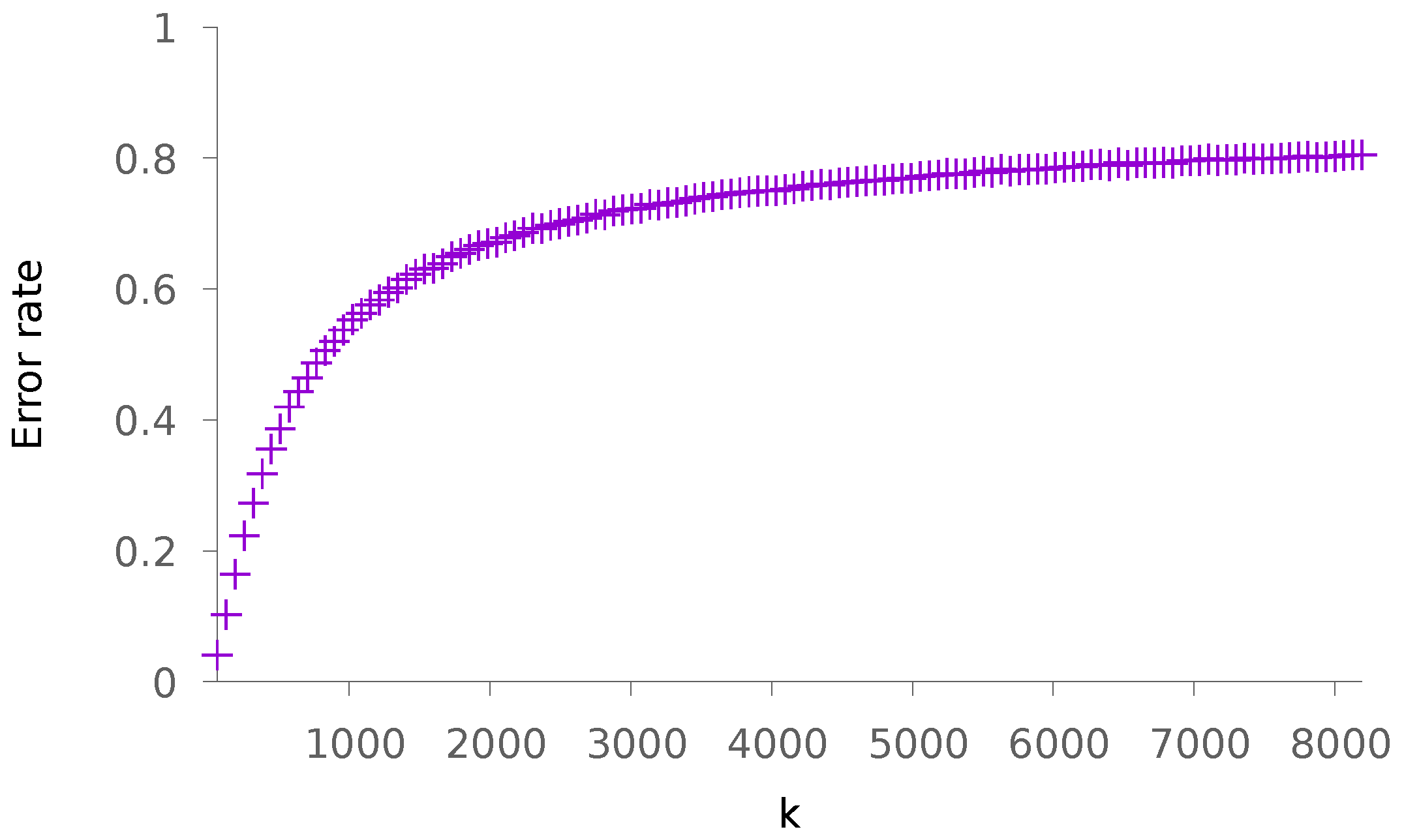
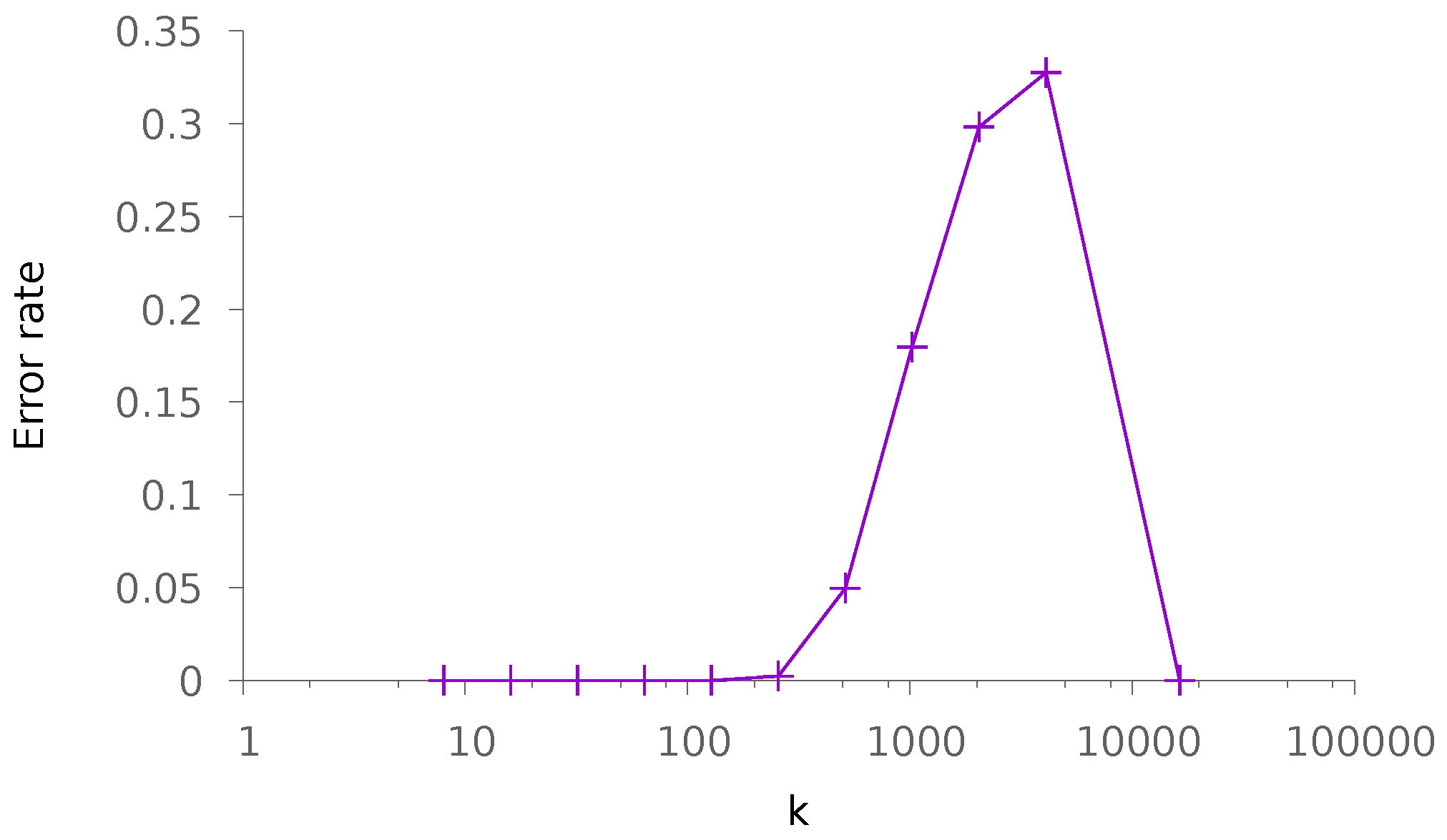
Our first two experiments consist of varying k and afterwards q while the other parameters are fixed. We choose the parameters $d=128$ and $c=8$. Figure 1 depicts the rate at which the highest score is not achieved by the class containing the query vector (we call it the error rate), as a function of k and for $q=10$. This function is obviously increasing with k and presents a high slope for small values of k, emphasizing the critical choice of k for applications.

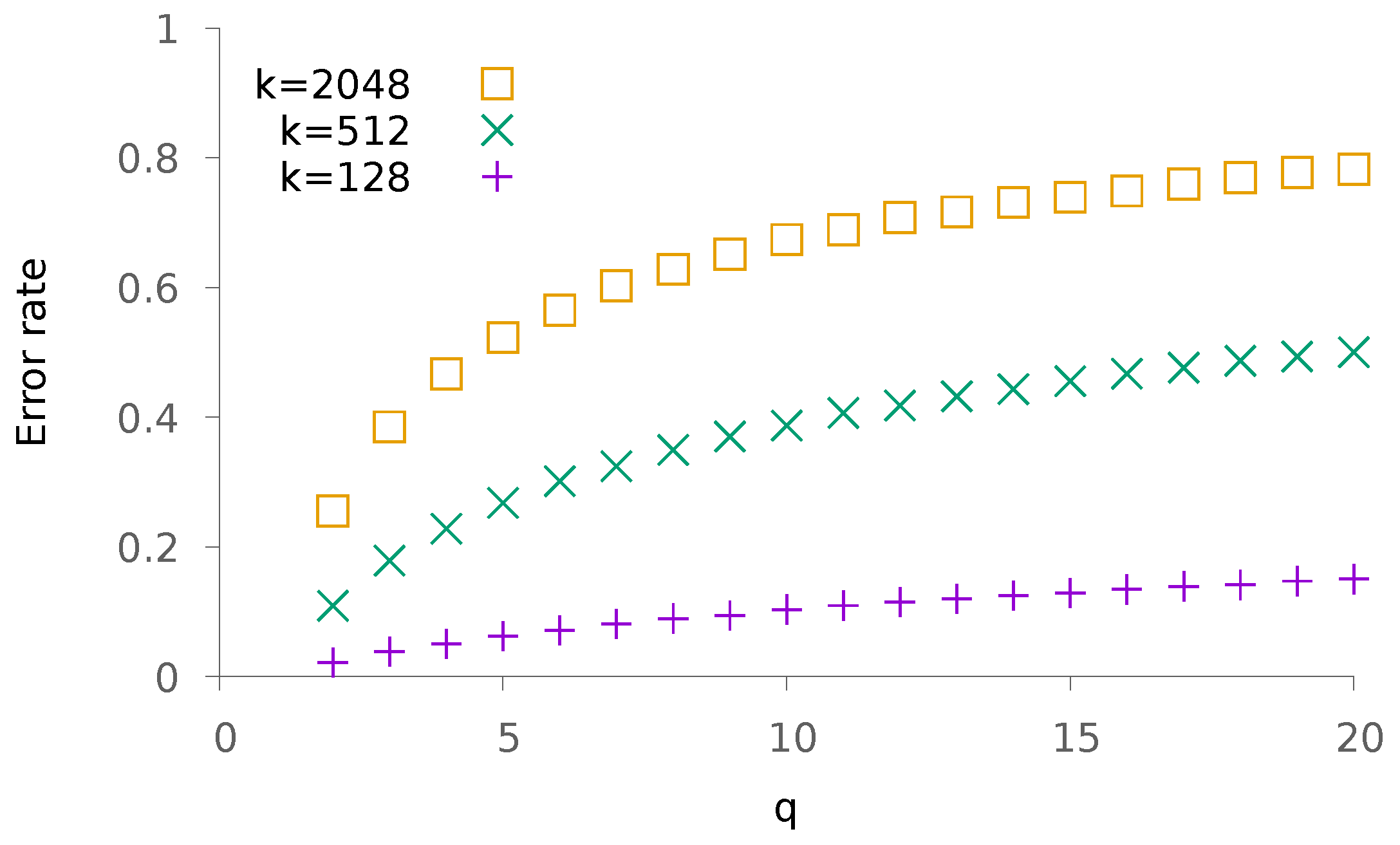
Figure 2 depicts the probability of error as a function of q, for various choices of k. Interestingly, for reasonable values of k the slope of the curve is not as dramatic as in Figure 1. When adjusting parameters, it seems thus more reasonable to increase the number of classes rather than the number of patterns in each class. This is not a surprising finding as the complexity of the process depends on q, but not on k.

Given data and their parameters c and d, a typical designing scenario would consist of finding the best trade-off between q and k in order to split the data in the different classes. Figure 3 depicts the error rate as a function of k when $n=kq$ is fixed. To obtain these points, we consider $c=8$, $d=128$ and n = 16,384. There are two interesting facts that are pointed out in this figure. First, we see that the trade-off is not simple as multiple local minima happen. This is not surprising as the decision becomes less precise and promissory, with larger values of k. As a matter of fact, the last point in the curve only claims the correct answer is somewhere in a population of 8192 possible solutions, whereas the first point claims it is one of the 64 possible ones. On the other hand, there is much more memory consumption for the first point where 256 square matrices of dimension 128 are stored, whereas only two of them are used for the last point. Second, the error rate remains of the same order for all tested couples of values k and q. This is an interesting finding as it emphasizes that the design of a solution is more about complexity vs. precision of the answer—in the sense of obtaining a reduced number of candidates—than it is about error rate.

Finally, in order to evaluate both the tightness of the bounds obtained in Section 3 and the speed of convergence, we run an experiment in which $c={log}_2(d)$, $q=2$. We then depict the error rate as a function of d and when $k=d^{1.5}$, $k=d^2$ and $k=d^{2.5}$. The result is depicted in Figure 4. This figure supports the fact that the obtained bound is tight, as illustrated by the curve corresponding to the case $k=d^2$ for which the error rate appears almost constant.

We ran the same experiments using co-occurrence rules as initially proposed in [7] (instead of adding contributions from distinct messages, we take the maximum). We observed small improvements in every case, even though they were not significant.

5.1.2. Dense Patterns

Let us now consider data to be drawn i.i.d. according to the distribution:

$$\mathbb{P}(x_i^{\mu }=1)=\frac{1}{2}=\mathbb{P}(x_i^{\mu }=-1);$$

recall that we then have three free parameters: d the dimension of patterns, k the number of patterns in each class and q the number of classes.

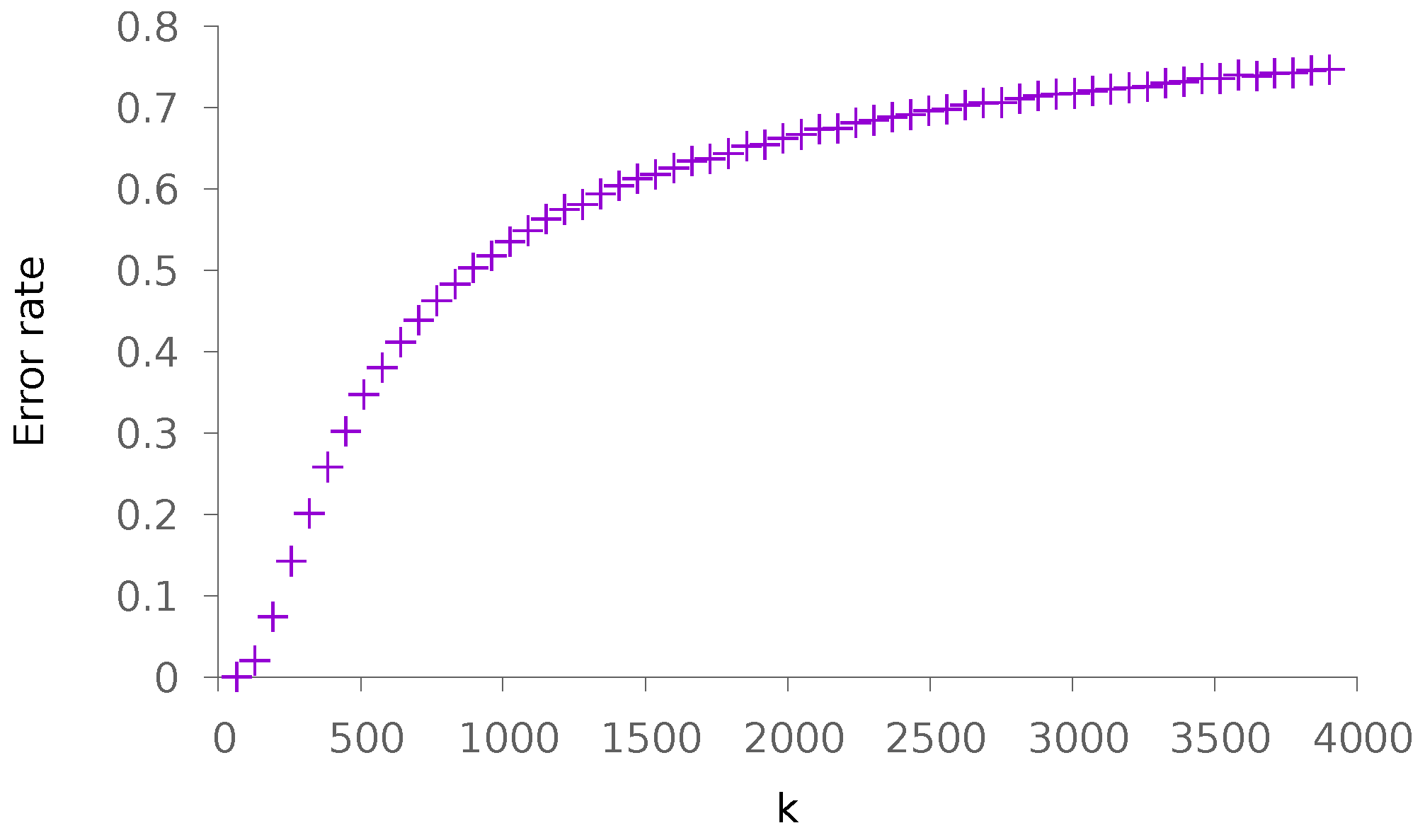
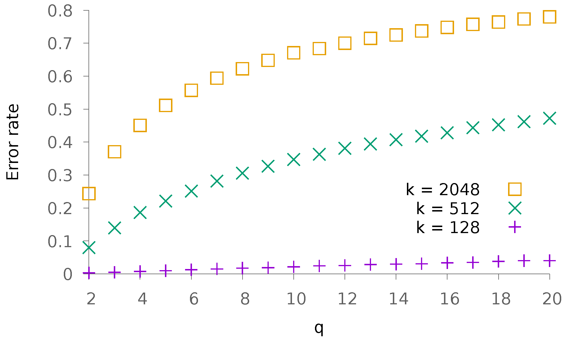
Again, we begin our experiments by looking at the influence of k (resp. q) on the performance. The obtained results are depicted in Figure 5 (resp. Figure 6). To conduct these experiments, we have chosen $d=64$. The global slope resembles that of Figure 1 and Figure 2.

Then, we consider the designing scenario where the number of samples is known. We plot the error rate depending on the choice of k (and thus, the choice of $q=n/k$). The results are depicted in Figure 7.

Finally, we estimate the speed of convergence together with the tightness of the bound obtained in Section 4. To do so, we choose k as a function of d with $q=2$. The obtained results are depicted in Figure 8. Again, we observe that the case $k=d^2$ appears to be a limit case where the error rate remains constant.

5.2. Real Data

In this section, we use real data in order to stress the performance of the obtained methods on authentic scenarios.

Since we want to stress the interest of using our proposed method instead of classical exhaustive search, we are mainly interested in looking at the error as a function of the complexity. To do so, we modify our method as follows: we compute the scores of each class and order them from largest to smallest. We then look at the rate for which the nearest neighbor is in one of the first p classes. With $p=1$, this method boils down to the previous experiments. Larger values of p allow for more flexible trade-offs of errors versus performance. We call the obtained ratio the recall@1.

Considering n vectors with dimension d, the computational complexity of an exhaustive search is $dn$ (or $cn$ for sparse vectors). On the other hand, the proposed method has a two-fold computational cost: first, the cost of computing each score, which is $d^{2}q$ (or $c^{2}q$ for sparse vectors), then the cost of exhaustively looking for the nearest neighbor in the selected p classes, which is $pkd$ (or $pkc$ for sparse vectors). Note that the cost of ordering the q obtained scores is negligible. In practice, distinct classes may have a distinct number of elements, as explained later. In this case, complexity is estimated as an average of elementary operations (addition, multiplication, accessing a memory element) performed for each search.

When applicable, we also compare the performance of our method with Random Sampling (RS) to build a search tree, the methodology used by PySparNN (https://github.com/facebookresearch/pysparnn), or Annoy (https://github.com/spotify/annoy). In their method, random sampling of r elements in the collection of vectors is performed; we call them anchor points. All elements from the collection are then attached to their nearest anchor point. When performing the search, the nearest anchor points are first searched, then an exhaustive computation is performed with corresponding attached elements. Finally, we also look at the performance of a hybrid method in which associative memories are first used to identify which part of the collection should be investigated, then these parts are treated independently using the RS methodology.

There are several things that need to be changed in order to accommodate real data. First, for non-sparse data, we center data and then project each obtained vector on the hypersphere with radius one. Then, due to the non-independence of stored patterns, we choose an allocation strategy that greedily assigns each vector to a class, rather than using a completely random allocation.

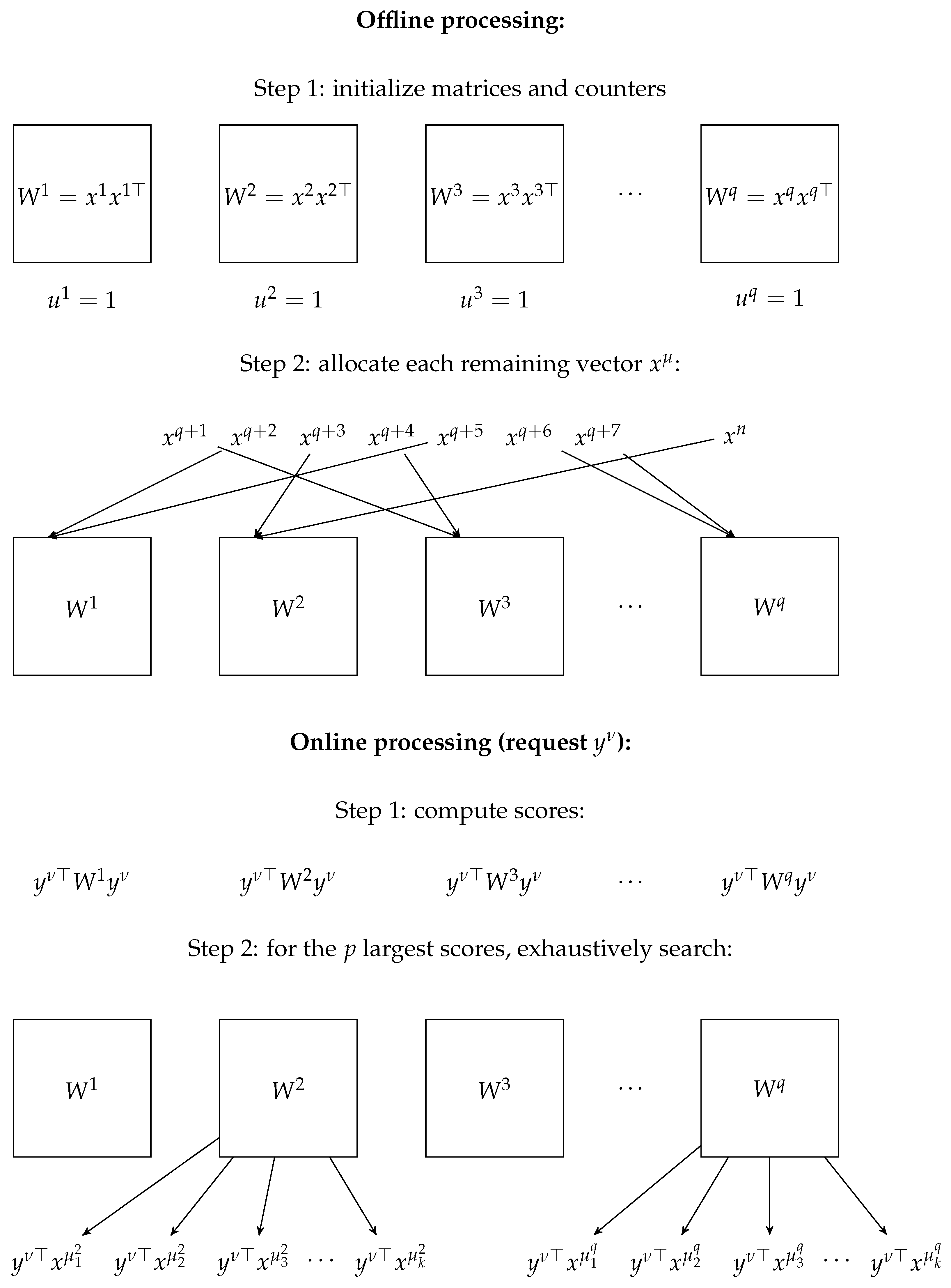
The allocation strategy we use consists of the following: each class is initialized with a random vector drawn without replacement. Then, each remaining vector is assigned to the class that achieves the maximum normalized score. Scores are divided by the number of items u currently contained in the class, as a normalization criterion. Note that more standard clustering techniques could be used instead. Figure 9 depicts all steps of the proposed method.

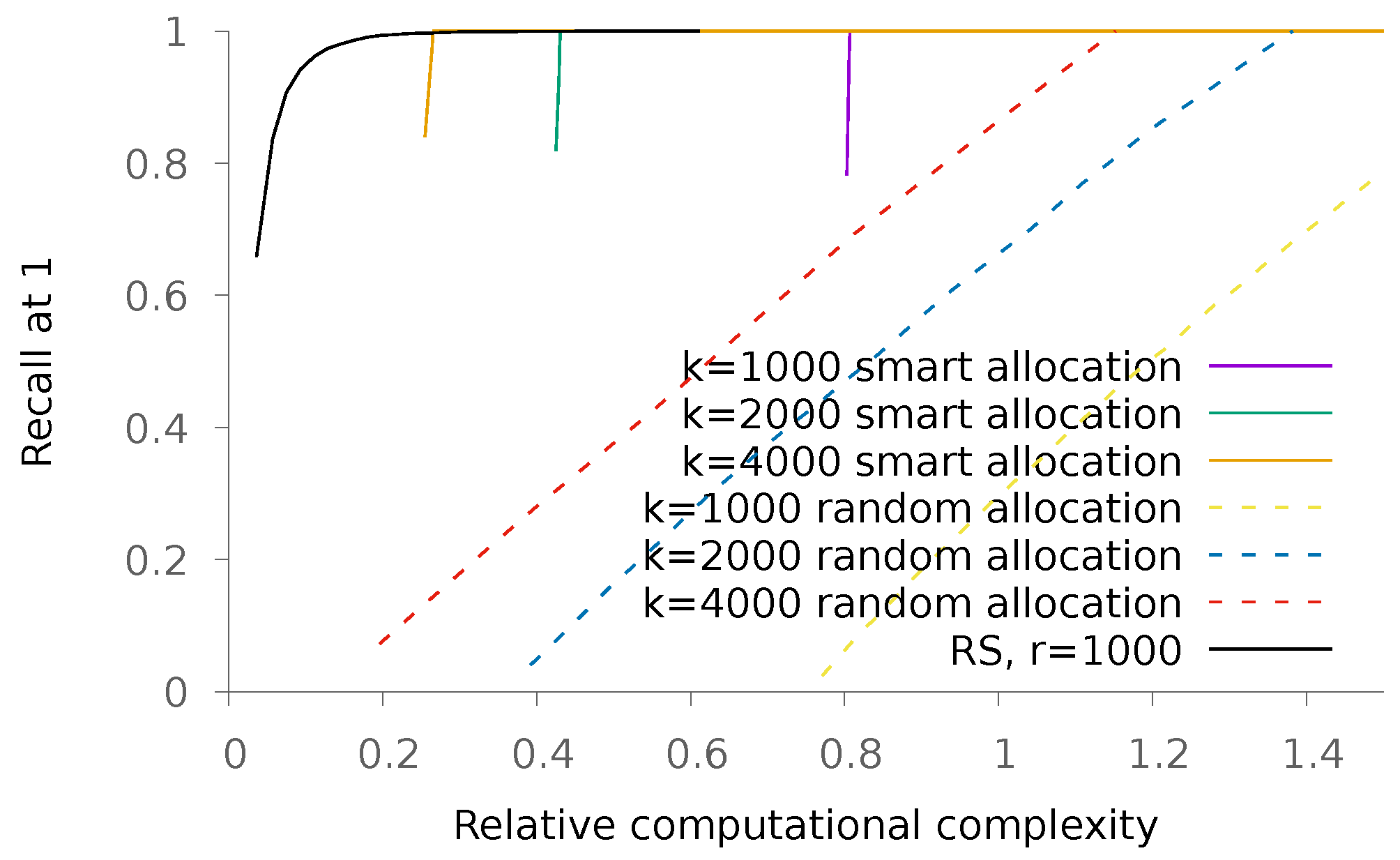
The interest of this allocation strategy is emphasized in Figure 10, where we use raw MNISTdata to illustrate our point. MNIST data consist of grey-level images with 784 pixels representing handwritten digits. There are 60,000 reference images and 10,000 query ones. For various values of k, we compare the performance obtained with our proposed allocation and compare it with a completely random one. We also plot the results obtained using the RS methodology. We observe that in this scenario where the dimension of vectors is large with respect to their number, associative memories are less performant than their RS counterparts.

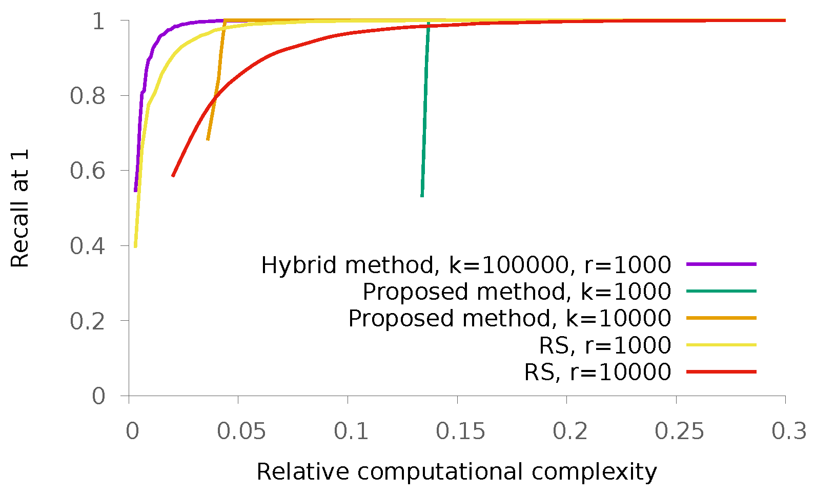
We also run some experiments on a binary database. It consists of Santander customer satisfaction sheets associated with a Kaggle contest. There are 76,000 vectors with dimension 369 containing 33 nonzero values on average. In this first experiment, the vectors stored in the database are the ones used to also query it. The obtained results are depicted in Figure 11.

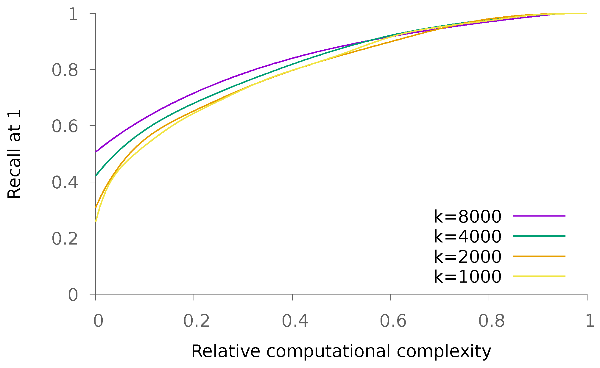
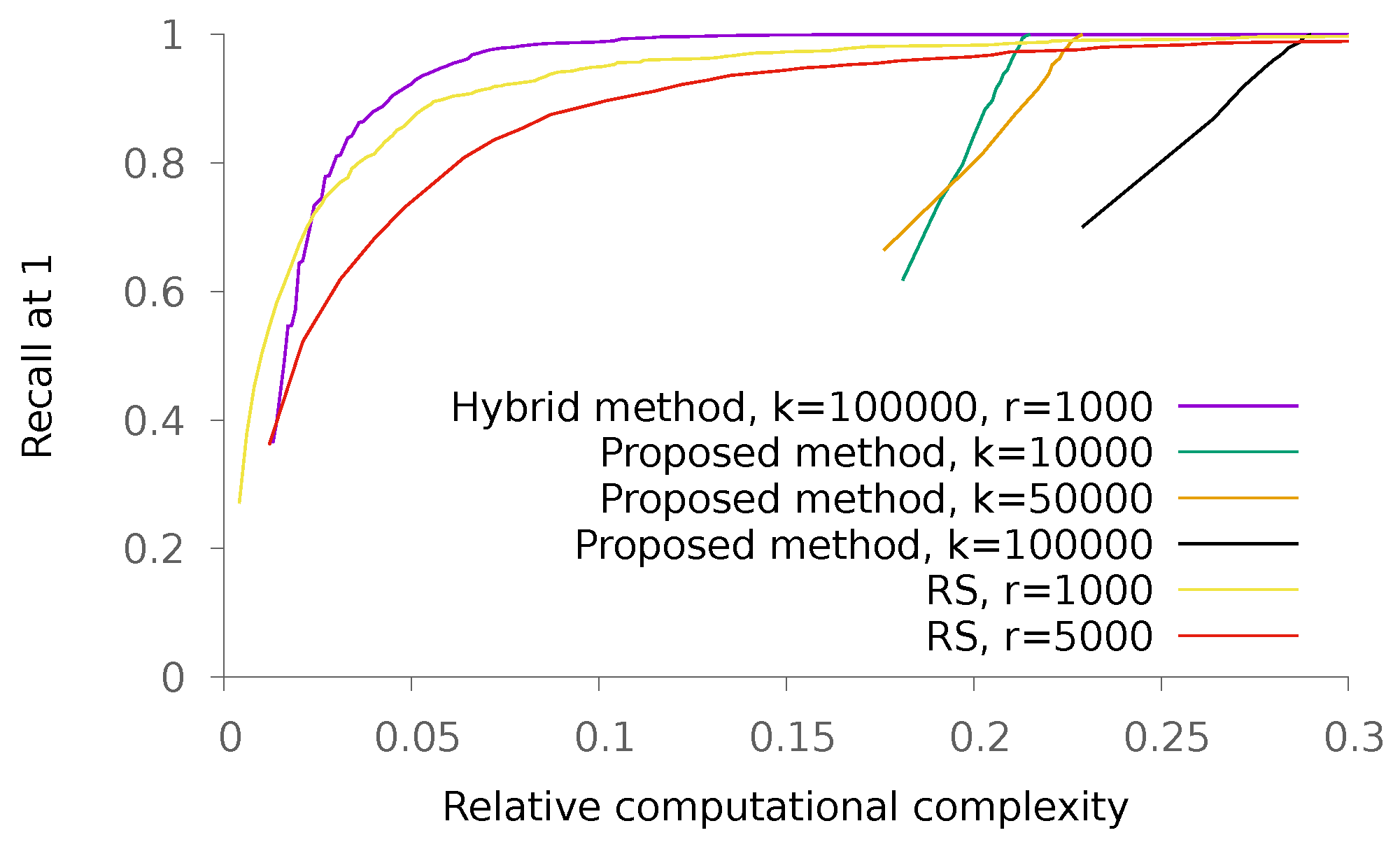
Then, we run experiments on the SIFT1M dataset (http://corpus-texmex.irisa.fr/). This dataset contains one million 128-dimension SIFT descriptors obtained using a Hessian-affine detector, plus 10,000 query ones. The obtained results are depicted in Figure 12. As we can see, here again, the RS methodology is more efficient than the proposed one, but we managed to find hybrid parameters for which performance is improved. To stress the consistency of results, we also run experiments on the GIST1Mdataset. It contains one million 960-dimensions GIST descriptors and 1000 query ones. The obtained results are depicted in Figure 13.

In

Table 1. Comparison of recall@1 and computation time for one scan (in ms) of the proposed method, kd-trees, K-means trees [1], ANN [16] and LSH [22] on the SIFT1M dataset for various targeted recall performances.

	Scan Time	Recall@1	Scan Time	Recall@1	Scan Time	Recall@1
Random kd-trees [1]	0.04	0.6	0.22	0.8	3.1	0.95
K-means trees [1]	0.06	0.6	0.25	0.8	2.8	0.99
Proposed method (hybrid)	0.17	0.6	0.25	0.8	1.1	0.99
ANN [16]	3.7	0.6	8.2	0.8	24	0.95
LSH [22]	6.4	0.6	11.1	0.8	28	0.98

, we compare the proposed method with random kd-trees, K-means trees [1], ANN [16] and LSH [22] on the SIFT1M dataset. To perform these measures, a computer using a i5-7400 CPU with 16 GB of DDR4 RAM was used. We used off-the-shelf libraries (https://github.com/mariusmuja/flann, http://www.cs.umd.edu/~mount/ANN/ and http://www.mit.edu/~andoni/LSH/). As expected, this table shows that important gains are expected when high precision is needed. On the contrary, gains are limited when facing low precision challenges. These limited gains are mainly explained by the fact the matrix computations are too expensive in the proposed method for scenarios with low precision.

In

Table 2. Comparison of the asymptotical complexity of the scan of one element in the search space for various methods, as a function of the cardinal n and the dimensionality d of the search space.

Technique	Scan Complexity	$\mathit{d}=\mathcal{O}(1)$	$\mathit{d}=\mathit{o}(log(\mathit{n}))$	$\mathit{d}=\mathbf{\Theta }({\mathit{n}}^{1/3})$	$\mathit{d}=\mathbf{\Theta }(\sqrt{\mathit{n}})$
Quantization	$\mathcal{O}(n)$	$\mathcal{O}(n)$	$\mathcal{O}(n)$	$\mathcal{O}(n)$	$\mathcal{O}(n)$
RS or K-means	$\mathcal{O}(d\sqrt{n})$	$\mathcal{O}(\sqrt{n})$	$o(log(n)\sqrt{n})$	$\mathcal{O}(n^{5/6})$	$\mathcal{O}(n)$
Proposed	$\mathcal{O}\left(q{d}^2+(n/q)d\right)$	$\mathcal{O}(\sqrt{n})$	$o(\sqrt{n}{log}^{3/2}(n))$	$\mathcal{O}(n)$	$\mathcal{O}(n)$
Hybrid scheme	$\mathcal{O}\left(q{d}^2+\left(k+n/q/k\right)d\right)$	$\mathcal{O}(n^{1/3})$	$o({log}^2(n)n^{1/3})$	$\mathcal{O}(n^{7/9})$	$\mathcal{O}(n)$

, we compare the asymptotical complexities of different methods. Note that we look at best cases for each method: for quantization techniques such as LSH, we consider that we can encode points using a number of bits that can be processed using only one operation on the given machine. For search space partitioning method, we always consider the balanced case where all parts contain an equal number of elements. This table shows that in terms of asymptotical complexity, the proposed method is not better than random sampling or K-means. This is because the cost of computing a score with the proposed scheme is larger than computing the distance to a centroid. Of course, this extra cost is balanced in practice by the fact that the proposed method provides a better proxy to finding the part of the space to search in, as emphasized in Figure 12 and Figure 13. Finally, the hybrid method obtains the best scores at each regime, thanks to the flexibility of its design.

6. Conclusions

We introduced a technique to perform approximate nearest neighbor search using associative memories to eliminate most of the unpromising candidates. Considering independent and identically distributed binary random variables, we showed there exists some asymptotical regimes for which both the error probability tends to zero and the complexity of the process becomes negligible compared to an exhaustive search. We also ran experiments on synthetic and real data to emphasize the interest of the method for realistic application scenarios.

A particular interest of the method is its ability to cope with very high dimension vectors, and even to provide better performance as the dimension of data increases. When combined with reduction dimension methods, there arise interesting perspectives on how to perform approximate nearest neighbor search with limited complexity.

There are many open ideas on how to improve the method further, including but not limited to using smart pooling to directly identify the nearest neighbor without the need to perform an exhaustive search, cascading the process using hierarchical partitioning or improving the allocation strategies.

References

- Muja, M.; Lowe, D.G. Scalable Nearest Neighbor Algorithms for High Dimensional Data. IEEE Trans. Pattern Anal. Mach. Intell. 2014, 36, 2227–2240. [Google Scholar] [CrossRef] [PubMed] [Green Version]
- Muja, M.; Lowe, D.G. Fast Approximate Nearest Neighbors with Automatic Algorithm Configuration. In Proceedings of the Fourth International Conference on Computer Vision Theory and Applications (VISAPP 2009), Lisboa, Portugal, 5–8 February 2009. [Google Scholar]
- Gong, Y.; Lazebnik, S. Iterative quantization: A procrustean approach to learning binary codes. In Proceedings of the 2011 IEEE Conference on Computer Vision and Pattern Recognition (CVPR), Colorado Springs, CO, USA, 20–25 June 2011; pp. 817–824. [Google Scholar]
- Jegou, H.; Douze, M.; Schmid, C. Product quantization for nearest neighbor search. IEEE Trans. Pattern Anal. Mach. Intell. 2011, 33, 117–128. [Google Scholar] [CrossRef] [PubMed] [Green Version]
- Datar, M.; Immorlica, N.; Indyk, P.; Mirrokni, V.S. Locality-sensitive hashing scheme based on p-stable distributions. In Proceedings of the Twentieth Annual Symposium on Computational Geometry, Brooklyn, NY, USA, 8–11 June 2004; pp. 253–262. [Google Scholar]
- Iscen, A.; Furon, T.; Gripon, V.; Rabbat, M.; Jégou, H. Memory vectors for similarity search in high-dimensional spaces. IEEE Trans. Big Data 2018, 4, 65–77. [Google Scholar] [CrossRef]
- Yu, C.; Gripon, V.; Jiang, X.; Jégou, H. Neural Associative Memories as Accelerators for Binary Vector Search. In Proceedings of the COGNITIVE 2015: 7th International Conference on Advanced Cognitive Technologies and Applications, Nice, France, 22–27 March 2015; pp. 85–89. [Google Scholar]
- Hopfield, J.J. Neural networks and physical systems with emergent collective computational abilities. Proc. Natl. Acad. Sci. USA 1982, 79, 2554–2558. [Google Scholar] [CrossRef] [PubMed]
- McEliece, R.J.; Posner, E.C.; Rodemich, E.R.; Venkatesh, S.S. The capacity of the Hopfield associative memory. IEEE Trans. Inform. Theory 1987, 33, 461–482. [Google Scholar] [CrossRef] [Green Version]
- Löwe, M.; Vermet, F. The storage capacity of the Hopfield model and moderate deviations. Stat. Probab. Lett. 2005, 75, 237–248. [Google Scholar] [CrossRef]
- Löwe, M.; Vermet, F. The capacity of q-state Potts neural networks with parallel retrieval dynamics. Stat. Probab. Lett. 2007, 77, 1505–1514. [Google Scholar] [CrossRef]
- Gripon, V.; Heusel, J.; Löwe, M.; Vermet, F. A comparative study of sparse associative memories. J. Stat. Phys. 2016, 164, 105–129. [Google Scholar] [CrossRef]
- Löwe, M. On the storage capacity of the Hopfield model with biased patterns. IEEE Trans. Inform. Theory 1999, 45, 314–318. [Google Scholar] [CrossRef]
- Newman, C. Memory capacity in neural network models: Rigorous lower bounds. Neural Netw. 1988, 1, 223–238. [Google Scholar] [CrossRef]
- Löwe, M.; Vermet, F. The Hopfield model on a sparse Erdos-Renyi graph. J. Stat. Phys. 2011, 143, 205–214. [Google Scholar] [CrossRef]
- Arya, S.; Mount, D.M.; Netanyahu, N.S.; Silverman, R.; Wu, A.Y. An optimal algorithm for approximate nearest neighbor searching fixed dimensions. J. ACM (JACM) 1998, 45, 891–923. [Google Scholar] [CrossRef] [Green Version]
- Tagami, Y. AnnexML: Approximate nearest neighbor search for extreme multi-label classification. In Proceedings of the 23rd ACM SIGKDD International Conference on Knowledge Discovery and Data Mining (KDD ’17), Halifax, NS, Canada, 13–17 August 2017; ACM: New York, NY, USA, 2017; pp. 455–464. [Google Scholar]
- He, K.; Wen, F.; Sun, J. K-means hashing: An affinity-preserving quantization method for learning binary compact codes. In Proceedings of the IEEE Conference on Computer Vision and Pattern Recognition, Portland, OR, USA, 23–28 June 2013; pp. 2938–2945. [Google Scholar]
- Weiss, Y.; Torralba, A.; Fergus, R.; Weiss, Y.; Torralba, A.; Fergus, R. Spectral Hashing. Available online: http://papers.nips.cc/paper/3383-spectral-hashing.pdf (accessed on 15 September 2018).
- Ge, T.; He, K.; Ke, Q.; Sun, J. Optimized product quantization for approximate nearest neighbor search. In Proceedings of the IEEE Conference on Computer Vision and Pattern Recognition, Portland, OR, USA, 23–28 June 2013; pp. 2946–2953. [Google Scholar]
- Norouzi, M.; Fleet, D.J. Cartesian k-means. In Proceedings of the IEEE Conference on Computer Vision and Pattern Recognition, Portland, OR, USA, 23–28 June 2013; pp. 3017–3024. [Google Scholar]
- Andoni, A.; Indyk, P. Near-optimal hashing algorithms for approximate nearest neighbor in high dimensions. In Proceedings of the 47th Annual IEEE Symposium on Foundations of Computer Science (FOCS’06), Berkeley, CA, USA, 21–24 October 2006; pp. 459–468. [Google Scholar]
- Norouzi, M.; Punjani, A.; Fleet, D.J. Fast search in hamming space with multi-index hashing. In Proceedings of the 2012 IEEE Conference on Computer Vision and Pattern Recognition (CVPR), Providence, RI, USA, 16–21 June 2012; pp. 3108–3115. [Google Scholar]
- Liu, Y.; Cui, J.; Huang, Z.; Li, H.; Shen, H.T. SK-LSH: An efficient index structure for approximate nearest neighbor search. Proc. VLDB Endow. 2014, 7, 745–756. [Google Scholar] [CrossRef]
- Kraska, T.; Beutel, A.; Chi, E.H.; Dean, J.; Polyzotis, N. The case for learned index structures. In Proceedings of the 2018 International Conference on Management of Data, Houston, TX, USA, 10–15 June 2018; pp. 489–504. [Google Scholar]
- Lindeberg, J.W. Über das Exponentialgesetz in der Wahrscheinlichkeitsrechnung. Ann. Acad. Sci. Fenn. 1920, 16, 1–23. [Google Scholar]
- Eichelsbacher, P.; Löwe, M. 90 Jahre Lindeberg-Methode. Math. Semesterber. 2014, 61, 7–34. [Google Scholar] [CrossRef]
- Eichelsbacher, P.; Löwe, M. Lindeberg’s method for moderate deviations and random summation. arXiv, 2017; arXiv:1705.03837. [Google Scholar]
- Demircigil, M.; Heusel, J.; Löwe, M.; Upgang, S.; Vermet, F. On a model of associative memory with huge storage capacity. J. Stat. Phys. 2017, 168, 288–299. [Google Scholar] [CrossRef]
Figure 1.
Evolution of the error rate as a function of k. The other parameters are , and .
Figure 2.
Evolution of the error rate as a function of q and for various values of k. The other parameters are and .
Figure 3.
Evolution of the error rate for a fixed number of stored messages 16,384 as a function of k (recall that ). The generated messages are such that and .
Figure 4.
Evolution of the error rate as a function of d. The other parameters are , and with various values of .
Figure 5.
Evolution of the error rate as a function of k. The other parameters are and .
Figure 6.
Evolution of the error rate as a function of q. We fix the value and consider various values of k.
Figure 7.
Evolution of the error rate for a fixed total number of samples as a function of k. The other parameters are 16,384 and .
Figure 8.
Evolution of the error rate as a function of d. In this scenario, we choose with various values of and .
Figure 9.
Illustration of the proposed method. Consider denotes a pattern of the collection to be searched and a request pattern. For any column vector x, denotes its transpose.
Figure 10.
Recall@1 on the MNISTdataset as a function of the relative complexity of the proposed method with regards to an exhaustive search, for various values of k and allocation methods. Each curve is obtained by varying the value of p.
Figure 11.
Recall@1 on the Santander customer satisfaction dataset as a function of the relative complexity of the proposed method with regards to an exhaustive nearest neighbor search, for various values of k. Each curve is obtained by varying the value of p.
Figure 12.
Recall@1 on the SIFT1Mdataset as a function of the relative complexity of the proposed method with regards to an exhaustive nearest neighbor search, for various values of k. Each curve is obtained by varying the value of p.
Figure 13.
Recall@1 on the GIST1Mdataset as a function of the relative complexity of the proposed method with regards to an exhaustive nearest neighbor search, for various values of k. Each curve is obtained by varying the value of p.