Dynamic Optimization Using Local Collocation Methods and Improved Multiresolution Technique

1
College of Astronautics, Nanjing University of Aeronautics and Astronautics, Nanjing 210016, China
2
Beijing Aerospace Automatic Control Institute, Beijing 100854, China
*
Author to whom correspondence should be addressed.
Appl. Sci. 2018, 8(9), 1680; https://0-doi-org.brum.beds.ac.uk/10.3390/app8091680
Submission received: 2 August 2018
/
Revised: 6 September 2018
/
Accepted: 14 September 2018
/
Published: 17 September 2018
(This article belongs to the Section Chemical and Molecular Sciences)
Abstract
:Dynamic optimization has wide applications in scientific and industrial researches. Multiresolution techniques provide an efficient way to solve dynamic optimization problems but have some disadvantages. An improved multiresolution technique is developed in this paper to overcome these disadvantages. The proposed technique consists of local collocation methods and a multiresolution-based mesh refinement method. New, generalized dyadic meshes are proposed to overcome the dyadic limitation, and the mesh refinement method is improved so that it can start with the coarsest generalized dyadic mesh. Additionally, the proposed technique involves a mesh refinement algorithm to remove the redundant mesh points in the constant control regions by analyzing the control slopes. The technique is applied to three chemical process control optimization problems and compared with other methods to demonstrate its effectiveness. Numerical results show that the proposed technique can solve chemical process control optimization problems accurately and efficiently and has advantages over other methods.
1. Introduction
Many scientific and industrial tasks, such as the optimal control of chemical processes and bioprocesses as well as control optimization in aerospace engineering, can be formulated as dynamic optimization problems (also named optimal control problems). Analytical solutions to dynamic optimization problems are difficult or even impossible to achieve. As a result, dynamic optimization problems are often solved using numerical methods. The most used numerical methods include direct methods [1,2,3] and indirect methods [4,5,6]. Indirect methods transform dynamic optimization problems into boundary value problems using the variational method or Pontryagin’s minimum principle. The primary advantage of indirect methods is that they satisfy the necessary optimality conditions. However, the boundary value problems are rather difficult to solve in most cases because they are very sensitive to initial values of adjoint variables. Direct methods discretize the control variables or both the control and state variables, and transform dynamic optimization problems into nonlinear programming (NLP) problems. The resulting NLP problems can be solved by standard NLP solvers such as the sparse nonlinear optimizer (SNOPT) [7] and the interior point optimizer (IPOPT) [8]. Some recommended literature reviews on numerical methods for solving dynamic optimization problems can be found in [9,10,11,12].
The use of direct methods to solve dynamic optimization problems has become more and more popular in recent years [3]. The major reason is that direct methods avoid the mathematical derivation of the necessary optimality conditions, which may be rather challenging for complex dynamic optimization problems. Furthermore, it is easy for direct methods to incorporate state and control constraints. Most of all, studies have reveal that direct methods are generally more robust with respect to inaccurate initial guesses, and therefore converge more easily. Direct methods can be further classified as direct shooting methods (also named control vector parameterization), which discretize only the control variables in the time horizon, and direct collocation methods, which discretize not only the control variables but also the state variables. The primary advantage of direct shooting methods is that the resulting NLP has a small number of variables [3]. The disadvantage of direct shooting methods is that the solution is very sensitive to the initial condition [3]. This high sensitivity can result in very nonlinear NLP constraints that are therefore very difficult to solve. Additionally, the nonlinearity in NLP constraints makes it difficult to construct accurate estimates of the first- and second-order derivative matrixes required for gradient-based optimization algorithms. The high dependence of the solution on the initial condition of shooting methods can be alleviated by multiple shooting methods [3,13,14] that divide the time horizon into a number of subintervals and then perform the shooting methods in each of the subintervals. Additional constraints are needed for multiple shooting methods to ensure continuity of state variables between adjacent subintervals. The NLP resulting from direct collocation methods, on the other hand, has many more decision variables because the methods discretize both the state variables and the control variables. However, the NLP problems from direct collocation methods are more robust to initial guesses of the decision variables and thus are easier to converge [2,15,16]. In aerospace engineering [3,12], both direct shooting methods and direct collocation methods have been widely used, and direct collocation methods are used even more often due to their excellent performance at solving complex dynamic optimization problems. In the optimization of chemical process or bioprocess control problems, direct shooting methods [14,17,18,19,20,21,22] appear to be used more often than direct collocation methods [3,23,24], especially when used in conjunction with mesh refinement methods. The present paper focuses on the application of direct collocation methods in conjunction with mesh refinement methods to chemical process and bioprocess optimization problems.
The solutions of many practical dynamic optimization problems are nonsmooth due to path or terminal constraints in the problem or nonsmooth problem formulations [25,26,27,28]. In order to solve these nonsmooth problems accurately using the direct collocation method, a globally dense mesh is not a good choice, because using very fine mesh may require large computational recourses, i.e., central processing unit (CPU) time and random-access memory (RAM). Furthermore, the large number of decision variables may make the resulting NLP problem poorly conditioned, which makes it very difficult or even impossible to solve by the NLP solvers [17]. Motivated by the desire to solve the dynamic optimization problems accurately while maintaining computational efficiency, many mesh refinement methods have been developed.
The mesh refinement methods are different for local collocation methods, which use a local polynomial to approximate the state dynamics, and global collocation methods (i.e., pseudospectral methods), which use a global polynomial to approximate the state dynamics. For local collocation methods, the mesh point distribution can be of any form needed. The mesh can be refined by minimizing the maximum local integration error [29] or by minimizing the maximum discretization error [30,31]. The multiresolution techniques (MRTs) of [25,26] refine the mesh by using a data compression algorithm. Zhao et al. [27] found that the MRTs of [25,26] cannot refine the mesh adequately in some cases, and proposed a mesh checking algorithm to avoid inadequate mesh refinement. In [28], an efficient mesh refinement method based on density functions was proposed to distribute the mesh points, but one must find an appropriate density function when using this method. There are also some other mesh refinement methods that were originally proposed for direct shooting methods but can also be used in conjunction with local collocation methods, e.g., the methods based on the wavelet analysis of the Lagrange functional gradients [18] or the control profiles [14,17], the method that analyzes the slope of control profiles [21], and the method that analyzes the sensitivity of the objective function with respect to discretized control variables [22]. For global collocation methods, the mesh points are determined by the roots of orthogonal polynomials, which means the mesh points cannot be freely distributed as those of local collocation methods. As a result, mesh refinement methods for global collocation methods are less flexible. The most used routine is to divide the dynamic optimization problems into many segments by introducing soft knots in the nonsmooth regions. The resulting mesh points become denser around the knots due to the special distribution of the mesh point of global collocation methods in each segment (denser towards the ends and sparse towards the middle). Furthermore, the control variables are not necessary continuous across the knots. The pseudospectral knotting method [32,33] solves nonsmooth dynamic optimization problems by either specifying the number and the location of the knots or automatically detecting the knots based on the control derivatives. The hp method [34,35] iteratively determines the width of each segment and number of mesh points in each segment by analyzing the midpoint residual or the state curvature. The ph method [36] is similar to the hp method [34,35] except that it tries to achieve the required accuracy by increasing the number of mesh point in each segment, or, if this fails, by increasing the number of segments. The method of [37] refines the mesh by analyzing the decay rates of Legendre polynomial. The capability to reduce the mesh size has been included in the latest mesh refinement methods [37,38]. However, it is not easy to determine the number and the locations of the knots needed to solve a nonsmooth dynamic optimization problem. In most cases, the abovementioned mesh refinement methods for global collocation methods generate a larger number of segments and mesh points [34,35,36,37,38].
Among the various mesh refinement methods, MRTs [25,26,27] are quite attractive because they only require simple analysis of the local interpolation error to refine the mesh, and avoid the complex analysis that is needed in other mesh refinement methods [14,17,18,28,29,30,31,34,35,36,38]. Moreover, the mesh point distribution of a local collocation method can be freely displaced according to the solution of the dynamic optimization problem, which is more flexible for accurately capturing the irregularities in the solution. In contrast, the mesh point distribution of a global collocation method is not so flexible because it is dictated by the roots of the first derivative of a certain global polynomial in each mesh interval. However, the MRTs of [25,26,27] still suffer from two disadvantages. First of all, the MRTs of [25,26] are based on dyadic meshes. Dyadic meshes consist of a hierarchy of meshes obtained from successively bisection of the unit interval [0, 1]. As a result of the dyadic bisection, the MRTs of [25,26] must start with an initial mesh consisting of 2j + 1 mesh points (where j is an integer). Although a generalized dyadic mesh has been proposed in [27] to overcome this limitation, the method of [27] must start with an initial mesh with a mesh size twice that of the coarsest mesh. This inconsistency between the initial mesh and the coarsest mesh makes it inconvenient to use in practical applications. Secondly, although the MRTs of [25,26,27] are quite efficient mesh refinement methods, they still generate some redundant mesh points in the solution. The efficiency of MRTs can be further improved if the redundant mesh points are removed. It is quite challenging to remove all the redundant mesh points, but it is possible to remove most of the redundant mesh points in the constant-control regions. Therefore, the other purpose of this paper is to improve the MRTs of [25,26,27] to overcome the abovementioned disadvantages. We first propose new generalized dyadic meshes so that the MRT can start with an initial mesh consisting of an odd number of mesh points rather than being limited to 2j + 1 mesh points. Furthermore, the MRT developed based on the new generalized dyadic meshes ensures that the initial optimization starts with the coarsest mesh. Finally, a method to remove the redundant points generated by MRTs in the constant control regions is developed by analyzing the control slopes. We currently only remove the redundant mesh points in the constant control regions because it is very common to have some constant control regions in the control solution for constrained dynamic optimization problems, e.g., the bang‒bang control problem.
The rest of this paper is organized as follows. In Section 2, the general continuous dynamic optimization problem is stated and the NLP formulations from the local collocation methods based on Runge‒Kutta (RK) discretizations are described. In Section 3, the improved MRT, which avoids the disadvantages of the MRTs of [25,26,27], is presented. In Section 4, the effectiveness of the method is demonstrated on three chemical process and bioprocess optimization problems and compared with other mesh refinement methods. In Section 5, the conclusion is summarized.
2. Problem Statement and Local Collocation Methods
Without a loss of generality, a dynamic optimization problem can be formulated as: minimizing the following Bolza cost functional:
subject to the state dynamic constraints
the boundary constraints (i.e., initial and terminal constraints)
and the inequality path constraints
where , , , , and , , , and . It should be noted that an equality path constraint can be decomposed into two inequality path constraints.
In addition to better numerical stability, it is more convenient to solve a dynamic optimization problem on the unit time interval [0, 1]. Therefore, the transformation is used to express the abovementioned dynamic optimization problem on the interval .
The local direct collocation methods based on RK discretizations [3] are used in the present research to transform the dynamic optimization problem into a NLP problem. The states, controls, and path constraints are discretized on a mesh with , and for . Let us denote and , and define the following sets:
The resulting NLP problem can be stated as: minimize the objective
subject to the following constraints:
where , U, , t0 and tf are the decision variables, , , , and . The intermediate variables , and are given by
The RK discretizations can be further classified according to the stage q. The commonly used discretization schemes include the trapezoidal scheme (q = 2), the Hermite‒Simpson scheme (q = 3), and the classical fourth-order RK scheme (q = 4). The parameters ρl, βl, and αlm are all known constants for a given discretization scheme, and their values are available in [3].
3. Improved Multiresolution Technique
In this section an improved multiresolution technique is described. The description contains three parts. First, new generalized dyadic meshes are proposed. Next, a method based on slope analysis is developed to remove the redundant mesh points in the constant control regions. Finally, the improved multiresolution technique is developed to refine the mesh.
3.1. New Generalized Dyadic Meshes
Generalized dyadic meshes have been proposed in [27], but the method of [27] must start with an initial mesh with a mesh size twice larger than that of the coarsest mesh, which is inconvenient to use. To avoid this shortcoming, new generalized dyadic meshes are described in this paper.
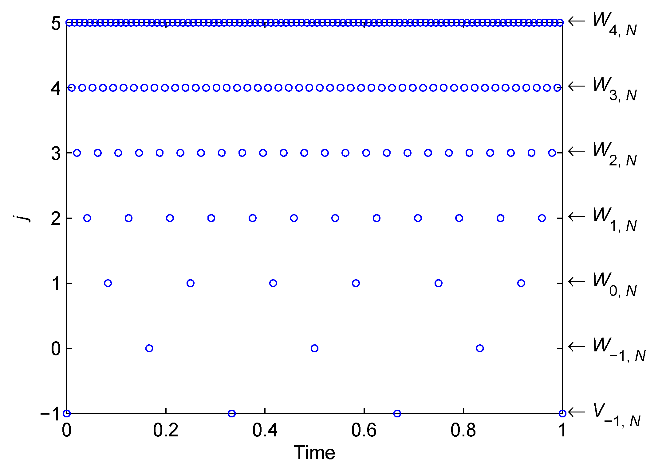
A uniform generalized dyadic mesh contains a hierarchy of mesh points that is obtained by successively bisection of a uniform initial mesh with N + 1 mesh points; that is:
where resolution level j, the spatial location k and the maximum resolution level Jmax are all positive integers. Note that N must be an even number because the minimum value of j is −1.
Let denotes the mesh points that belong to ,
It is easy to know , because
Figure 1 shows an example of a generalized dyadic mesh with N = 6 and Jmax = 5. It should be noted that the generalized dyadic meshes determined by Equations (11) and (12) is compatible with the dyadic mesh given in [25,26], where N must be equal to 2j. The generalized dyadic mesh of this paper avoids dyadic restriction and therefore is more convenient to use. In addition, as can be seen in Section 3.3, the improved multiresolution technique based on this new generalized dyadic mesh avoids the inconsistency between the initial mesh and the coarsest mesh.
3.2. Slope Analysis of Control Variable
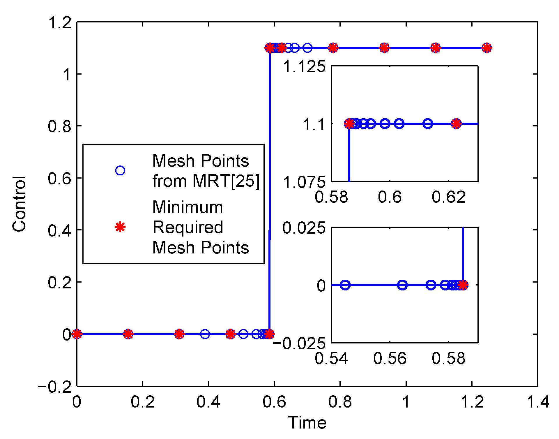
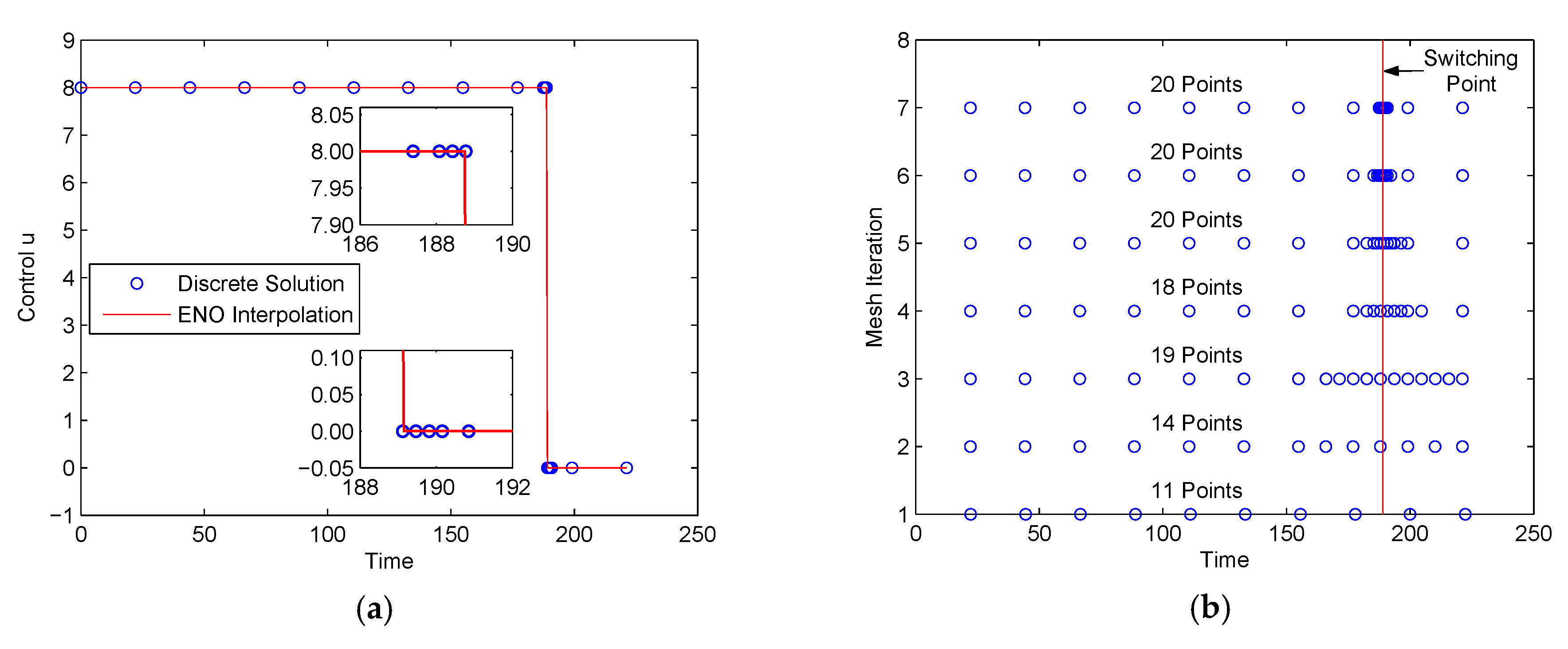
As an example, Figure 2 shows a bang‒bang control solution solved by the MRT [25], which refines the mesh using the data compression algorithm based on dyadic meshes. The method started with a uniform initial mesh consisting of 23 + 1 points and terminated with a nonuniform final mesh consisting of 30 points. Although the method generated only 30 mesh points, there are still some redundant mesh points in the solution. As shown in Figure 2, the control profile can be captured accurately by the nine initial mesh points and the two mesh points that are adjacent to the bang‒bang switching location. These theoretical minimum required mesh points are denoted by the symbol * in Figure 2. In other words, most of the other 11 mesh points are redundant and thus can be removed to further improve the computational efficiency of the MRT.
The redundant mesh points in Figure 2 can be removed by analyzing the slopes of the control variable. The left slope of the control variable at the mesh point τk, k = 1, 2, …, Nτ − 1, is
where and are the control values at the mesh points and , respectively.
The right slope of the control variable at the mesh point τk, k = 1, 2, …, Nτ − 1, is
If both the left slope and the right slope at a mesh point are zero, then the mesh point is determined as a redundant point and should be removed. The slope analysis is repeated for all the mesh points to remove the redundant ones. It should be noted that the initial mesh points should not be removed. Additionally, the mesh points of the highest resolution in the mesh should also be kept in the mesh to robustly capture the nonsmooth changes in the control profile.
The abovementioned slope analysis procedure is responsible for removing the redundant mesh points generated by the MRTs of [25,26,27], although it can only remove the redundant mesh points in the constant control regions. This function is useful because it is very common to have some constant control regions in the control profile(s), especially for the constrained dynamical optimization problems. It is also useful but more challenging to remove the redundant mesh points in the non-constant control regions, which is beyond the scope of the present paper.
3.3. Improved Multiresolution Technique
Several parameters must be specified for the improved multiresolution technique; that is, the parameter N for the initial mesh V0, N; the mesh refinement tolerance ε, the mesh resolution Jmax and the mesh refinement iteration Imax (Imax ≥ Jmax + 1. The default value is Jmax + 1). The proposed improved multiresolution technique contains three major steps. First of all, the dynamic optimization problem is transcribed into an NLP problem using one of the RK discretization schemes described earlier. Second, set I = 1, initialize Gold = V0, N, and let χold denote the initial guesses for the NLP decision variables. Then, the improved multiresolution technique proceeds as follows.
- (1)
- Solve the discretized dynamic optimization problem on mesh Gold with χold as the initial values for the NLP variables. If I ≥ Imax, terminate; otherwise move on to the next step.
- (2)
- Refine the mesh Gold via the following steps (step 2a to step 2f):
- (a)
- Let .
- (b)
- Initialize Gint = V0, N, , and j = −1.
- (c)
- Mesh refinement algorithm I (MRA-I).
- (d)
- Mesh refinement algorithm II (MRA-II).
- (e)
- Mesh refinement algorithm III (MRA-III).
- (f)
- The refined mesh is Gnew = Gint, with the control values Φnew = Φint.
- (3)
- Set I = I + 1. If Gnew is the same as Gold, stop; otherwise, renew χold by interpolating the NLP solution that is solved in step 1 on Gnew, set Gold = Gnew, and go to step 1.
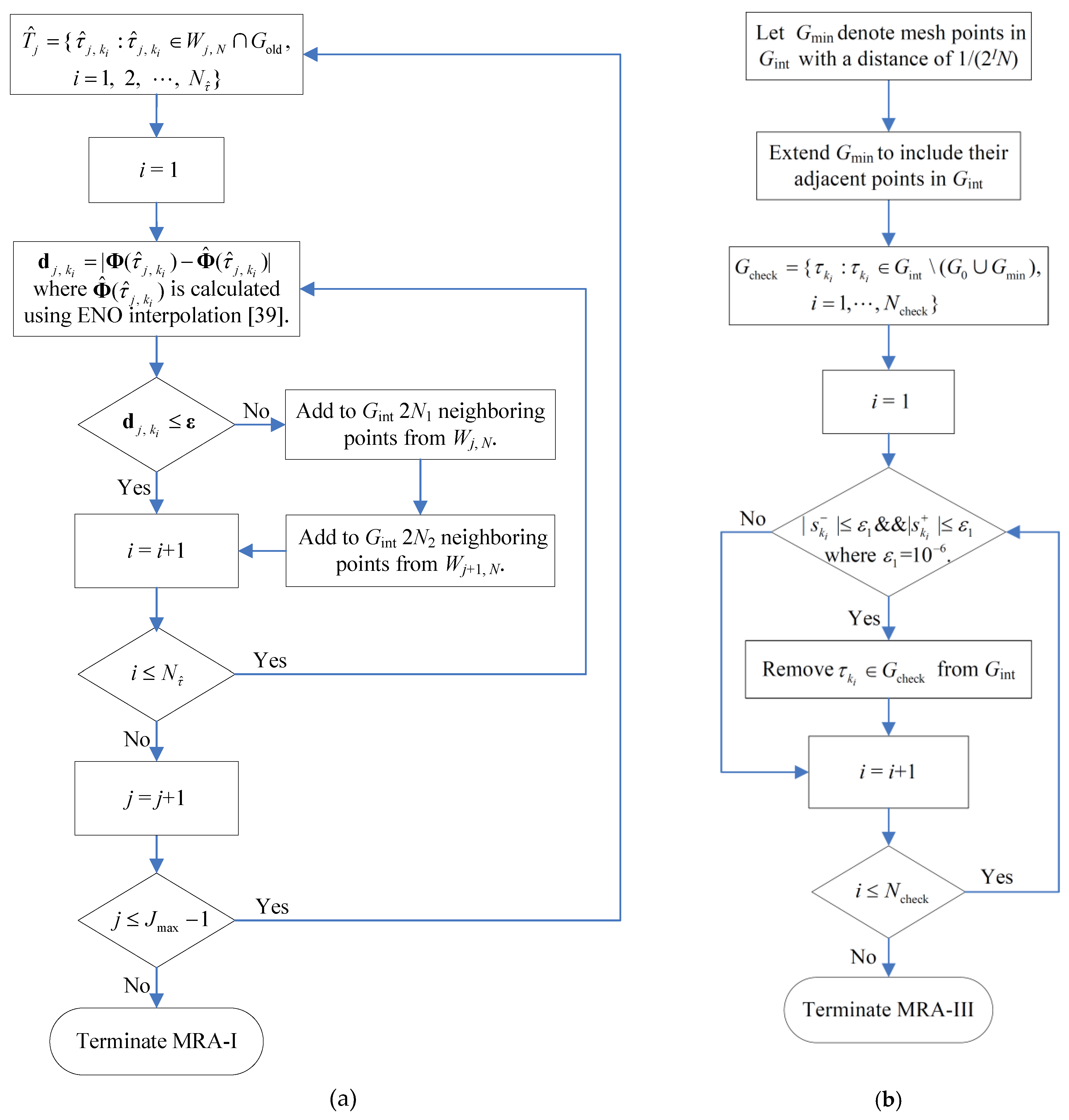
The MRA-I in step 2c is similar to the MRT of [25] except that the MRA-I is based on the new generalized dyadic meshes described in Section 3.1. Because of this improvement, the MRA-I overcomes the dyadic limitation on the number of points in the initial mesh and the inconsistency between the initial mesh and the coarsest mesh. Figure 3a gives the flowchart of MRA-I. It should be noted that the interpolated function values in Figure 3a is calculated from the neighboring points of in Gint (but not including itself) and the corresponding function values in Φint using the pth-order essentially non-oscillatory (ENO) interpolation [39].
The MRA-II in step 2d is used to overcome the omission or failure of mesh refinement in MRA-I. It was found that the multiresolution technique may fail to refine the mesh adequately in some special regions if only the control variables are used in mesh refinement [27]. The present paper uses the mesh checking algorithm of [27] as MRA-II. The mesh checking algorithm checks the interpolation errors at all the points in the mesh refined by MRA-I, and adds some mesh points where needed. The details of the mesh checking algorithm are given in [27].
The MRA-III of step 2e is responsible for removing the redundant mesh points in the constant control regions by analyzing control slopes. Figure 3b gives the flowchart of MRA-III.
It should be noted that the MRTs of [25,26] are based on dyadic meshes and are similar to MRA-I. They do not involve MRA-II and MRA-III. As a result, the MRTs of [25,26] suffer from dyadic restriction on initial meshes. Furthermore, they may fail to refine the mesh adequately in some special regions and generate some redundant mesh points in the constant control regions. Although the MRTs of [27] are based on generalized dyadic meshes and involve MRA-II, they suffer from the inconsistence between the initial mesh and the coarsest mesh, and still generate some redundant points in the constant control regions. The method of the present paper overcomes these shortcomings by involving the algorithms MRA-I, MRA-II, and MRA-III.
4. Numerical Examples
In this section, the improved multiresolution technique is tested on three examples of different complexity to demonstrate its effectiveness. The first example is a simple chemical reaction problem [30], the second is a drug displacement problem [40], and the third is a complex semi-batch reactor control problem [14,20]. In all three examples, it is shown that the proposed method starts with the coarsest mesh and is able to remove most of the redundant mesh points in the constant control regions. In the last two examples, it is shown that the proposed method can start with a mesh with the number of mesh points not limited to 2j + 1. Additionally, all the examples show that the chemical process optimization problems can be solved accurately and efficiently by the local collocation methods and the improved multiresolution technique.
In each example, the Hermite‒Simpson scheme (q = 3) [3] was used to transform the dynamic optimization problem into a NLP problem. The NLP problem was then solved by SNOPT 7 [7] with the first derivatives provided by INTLAB 5.5 [41]. The parameters used in the mesh refinement algorithm were p = 2, N1 = 1 and N2 = 1. Comparisons with the original multiresolution technique and the hp adaptive method were also provided in the third example, where it is seen that the improved multiresolution technique leads to fewer mesh refinement iterations and smaller mesh size. The computing platform was a MacBook Air (1.6 GHz Intel Core i5-5250U and 4 GB 1600 MHz DDR3 RAM) running Windows 10 Enterprise 10240 and MATLAB R2009a.
4.1. Simple Chemical Reaction Problem
We first apply the proposed method to maximize the final amount of product in a simple two-stage chemical reaction [26,30]. The problem is expressed as follows: minimize
subject to the state dynamics
the initial conditions
and the control bounds
where ρ and k are constants, ; is fixed at .
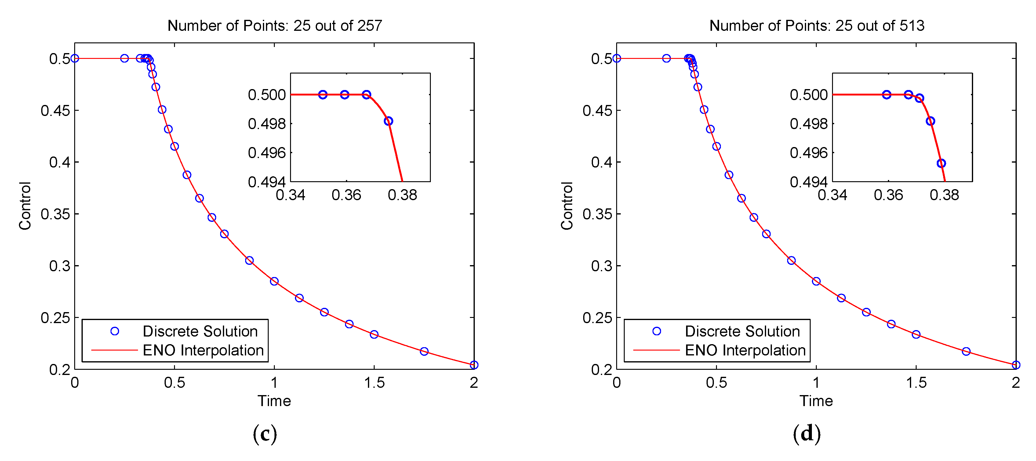
We solved this problem using the proposed method with N = 8 and Jmax = 6. The mesh refinement tolerance was ε = 1.0 × 10⁻³. The method stopped after seven iterations. The time history of the control u for iterations 1, 2, 6, and 7 is shown in Figure 4, where the mesh points are the discrete control solutions, and the solid lines are obtained using the pth-order ENO interpolation.
It is seen in Figure 4a that the proposed method started with the coarsest mesh and was able to remove most of the redundant mesh points in the constant control region, as shown in Figure 4c,d. As a result, the method used only 25 mesh points from the maximum of 513 points at the finest mesh V6, N. The objective function value was 0.308132135. The total CPU time required to solve this problem was 1.73 s. In contrast, the problem was also studied in [30] where the mesh was refined using a method by minimizing the maximum discretization error. The method of [30] generated 62 mesh points and achieved an objective value of 0.308132178. It is seen that the proposed method achieved nearly the same objective value as the method of [30] but used a much smaller mesh size, which therefore has the potential to reduce the computational cost.
4.2. Drug Displacement Problem
In this example, we consider a time-optimal drug displacement problem [40], where it is shown that the proposed method is also applicable for the optimizing continuous chemical process. The problem simulates the drug interaction of the two drugs warfarin and phenylbutazone in a patient’s bloodstream. The problem is to control the rate of infusion of the pain-killing drug phenylbutazone so that the desired level of two drugs can be reached in the minimum time and the concentration of warfarin does not rise above a toxic level during the dynamic process.
This problem is expressed as: minimize the final time
subject to the state dynamics
where the state variables x1 and x2 are the concentrations of warfarin and phenylbutazone respectively, u is the control variable, and C1, C2, C3, and C4 are defined as follows:
The initial and the terminal conditions are
The control bounds are
The path constraint on the concentration of warfarin is
where α is the allowable upper limit for the concentrations of warfarin, and α = 0.026.
We solved this problem using the proposed method with N = 10, Jmax = 6 and ε = 0.05. Note that the parameter N was specially chosen to not equal 2j (j is an integer). We first solved the problem without considering the path constraint of Equation (24). The method stopped after seven iterations. Figure 5 shows the control solution and the mesh refinement history. It is seen in Figure 5a that the control solution was a bang‒bang solution and the switching point in the control profile was captured accurately, as shown in the two insets in Figure 5a. The mesh point history in Figure 5b shows that the mesh size did not grow much as the mesh refinement proceeded, because most of the unnecessary points were removed. As a result, the method used only 20 points of the maximum of 641 points at the finest resolution mesh V6, N. The objective function value was J* = 221.2748 s, which is slightly smaller than the value of 221.4661 s obtained in [40] using the indirect multiple shooting algorithm. The CPU time required to solve this problem was 0.98 s.
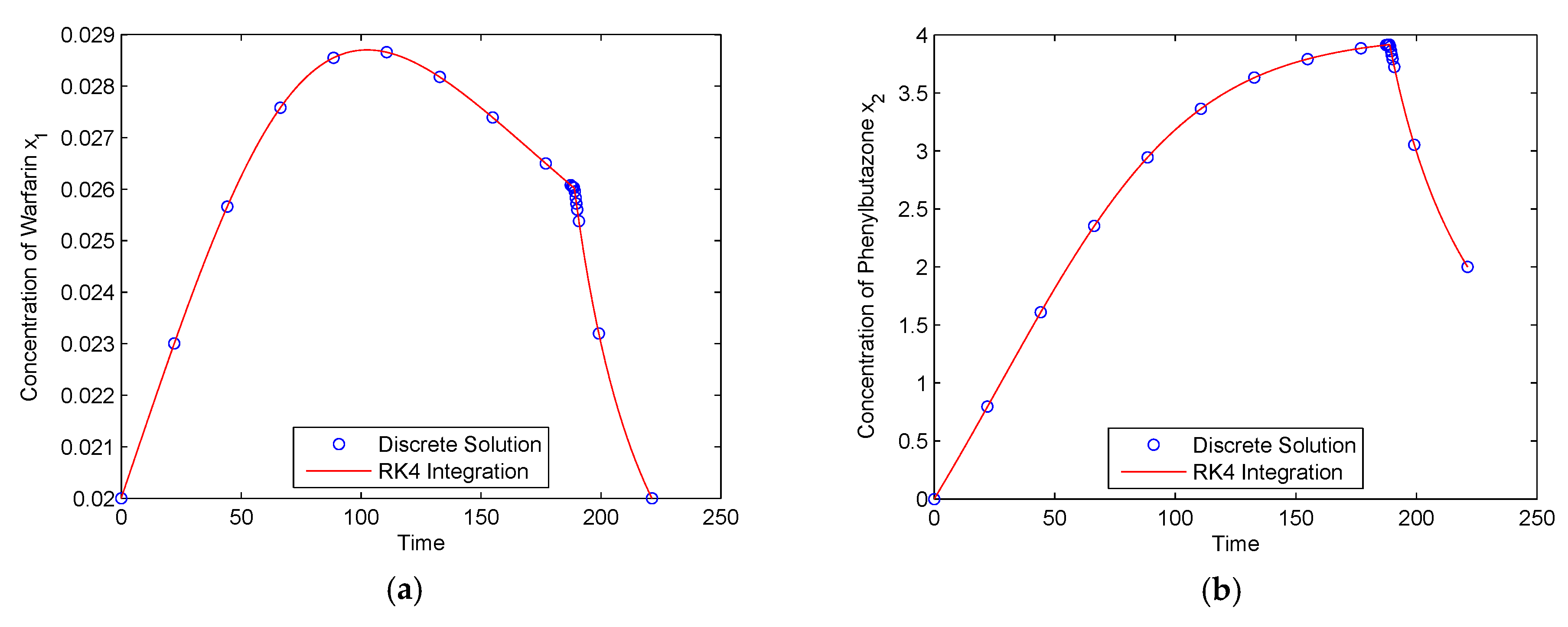
The time histories of the two states are shown in Figure 6. The circle markers denote the discrete solutions, and the solid lines are the results obtained by integrating of the state dynamics along the optimal control solution using the classical fourth-order RK method. It is seen in Figure 6 that the two results are in excellent agreement, and both the two states achieved the required values at the terminal time. It should be noted that the maximum concentration of warfarin exceeded the allowable upper limit, because the path constraint of Equation (24) was not considered.
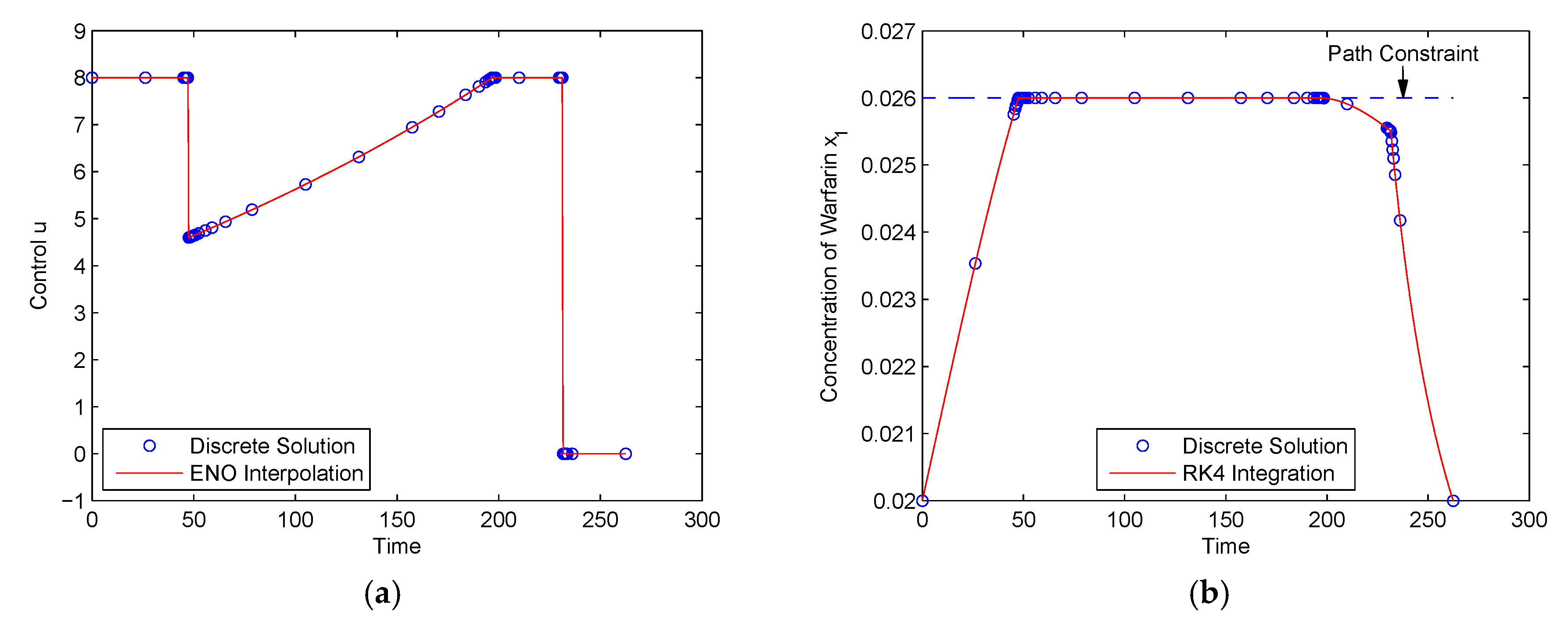
We then solved this problem again with the path constraint of Equation (24) considered. The method stopped after seven iterations and selected 45 mesh points from V6, N. The control solution and the constrained state variable are shown in Figure 7. As shown in Figure 7a, although the control solution became much more complex, all the switching points in the control profile were captured accurately. It is seen in Figure 7b that the concentration of warfarin strictly satisfied its path constraint. The objective value was J* = 262.4140 s, which is again slightly smaller than the value of 262.637 s obtained in [40] using the indirect multiple shooting algorithm.
4.3. Williams‒Otto Semi-Batch Reactor Control Problem
In this example, the proposed method was applied to the control of a more complex semi-batch reactor problem, i.e., the Williams‒Otto semi-batch reactor. The problem is a benchmark problem which has been extensively studied in literatures [5,14,17,20,42]. The dynamic optimization problem is stated as: find the optimal control u(τ) = [TW(τ), FB,in(τ)]T, where TW(τ) is the cooling water inlet temperature and FB,in(τ) is the feed flow rate of a reactant that maximizes the objective
The state dynamic equations are
where the expressions of r1, r2 and r3 are given by
The initial values of the state variables and the values of the parameters are given in [14]. It should be noted that the time horizon in (26) has been scaled to τ [0, 1] by the final time tf = 1000 s.
The path constraints on the reactor temperature are
The terminal constraint on the reactor volume V is
The control bounds are
We solved this problem using the proposed method with N = 20, Jmax = 7 and ε = 1.0 × 10⁻¹. Again, the parameter N was specially chosen to be not equal to 2j (j is an integer). The method stopped after eight iterations, and selected 101 points from the maximum of 2561 points at the finest mesh V7, N. Figure 8 shows the optimal control solutions solved by the proposed method. It is seen that the control switching points were all captured accurately, although the method removed most of the redundant mesh points in the constant control regions. The mesh refinement history is shown in Figure 9, where the vertical lines indicate the switching points in the control solutions. It is seen that the method started with the coarsest mesh and the mesh size did not increase much during the mesh refinement iterations because the redundant mesh points were removed during the refinement. The objective value obtained from the proposed method was −4768.313612, which is very near the value of −4768.314 calculated by an indirect multiple shooting method [5].
The time histories of the two constrained state variables, i.e., the reactor temperature TR(t) and the reactor volume V(t), are displayed in Figure 10, where the circle markers are the discrete solutions and the solid lines are the results obtained by integrating the state dynamics along the optimal control solutions using the classical fourth-order RK method. It is seen that the discrete solutions and the integration results are in good agreement. Furthermore, both the state variables strictly satisfy their constraints. These results demonstrate the effectiveness of the method.
For comparison, we also solved this example by ignoring the mesh refinement algorithm MRA-III, which is responsible for removing the redundant mesh points generated by MRA-I and MRA-II in the constant control regions. In this case, the method became similar to the MRTs described in [25,26,27], except that the methods of [25,26] must start with 2j + 1 mesh points and the method of [27] must start with a mesh size twice larger than that of the coarsest mesh. The technique terminated after eight iterations and the optimal control solutions are given in Figure 11. The objective function value is 4768.313475. It is seen that both the control solutions and the objective function are nearly the same as those obtained when MRA-III is not ignored, but there are considerable redundant mesh points in the constant control regions. The technique selected 162 points from the maximum of 2561 points at the finest mesh V7, N. The mesh size is 1.6 times larger than that obtained when MRA-III is not ignored. The total CPU time for this example is 21.5 s. Again, this example demonstrates the advantages of the proposed method.
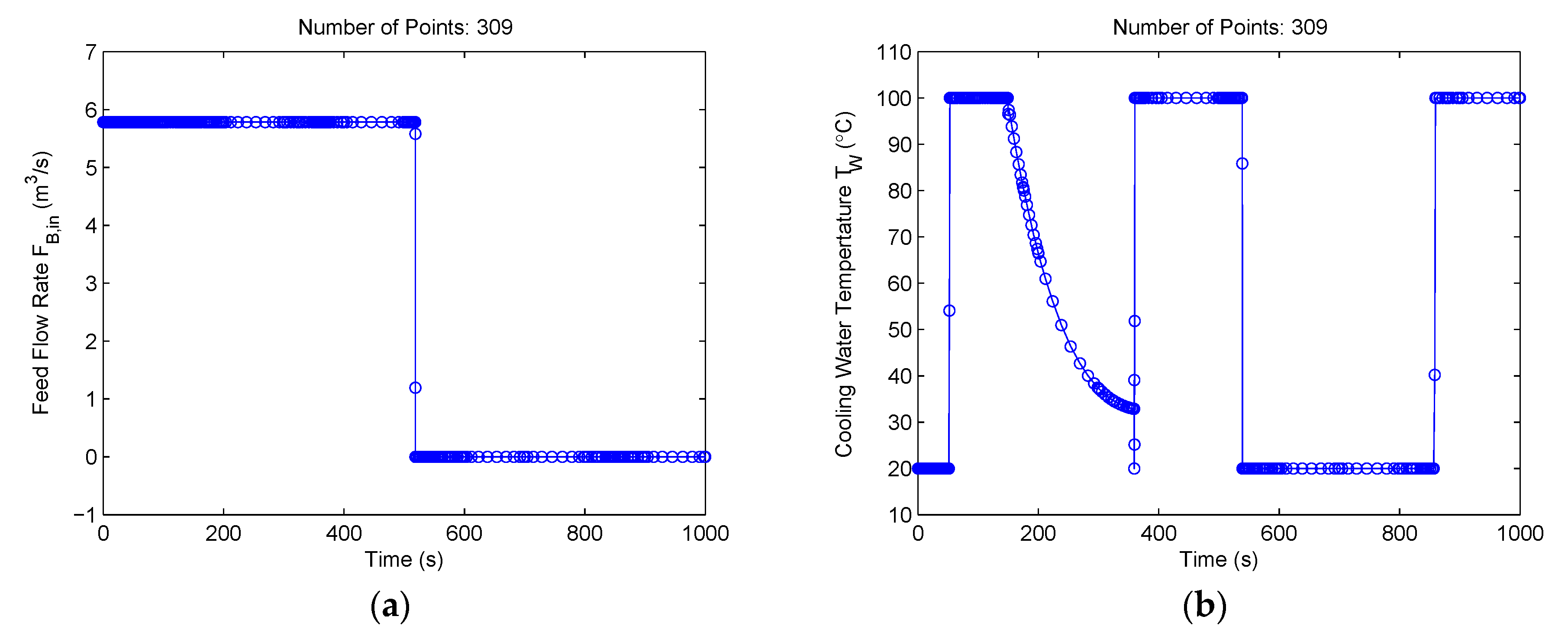
Additionally, the method of this paper was compared with the hp-adaptive pseudospectral method [35], which adjusts both the width and the number of mesh points in each segment by analyzing the state curvature. The optimality and feasibility tolerances for SNOPT were identical to those used in our method. The hp-adaptive method was executed using the open-source optimal control software GPOPS II 1.0 [43]. The hp-adaptive method terminated after 13 iterations and used 309 mesh points at the final iteration. The control solutions are shown in Figure 12. The obtained objective function value was −4768.313425. It is seen in Figure 12 that the control solutions are similar to the results obtained from our method. However, the hp-adaptive method required 1.6 times more mesh iterations and generated a 3.06-fold larger mesh size when compared with our method. The CPU time required by the hp-adaptive method was 21.1 s, although GPOPS II used a quite efficient method to explore the NLP sparsity and calculate the NLP derivatives [44]. Furthermore, it is seen in Figure 12b that there is some noise in the cooling water temperature profile. The comparisons again demonstrate the advantages of the proposed method.
The mesh refinement results obtained from the three abovementioned methods are summarized in Table 1. Although the CPU times are listed in Table 1 for reference, it should be noted that the CPU times are affected by other many factors (e.g., the way to calculate the NLP derivatives) in addition to the mesh size and the mesh iterations. Therefore, it is more reasonable to compare the efficiencies of different mesh refinement methods by comparing the mesh iterations and the mesh size. It is seen in Table 1 that the proposed method generated a much smaller mesh size and required fewer mesh iterations when compared with other mesh refinement methods, so the proposed method is more efficient than other methods. The objective values from different methods are comparable and are all near to the value from the indirect method.
5. Conclusions
An improved multiresolution technique has been developed in this paper for solving dynamic optimization problems. The technique is based on local direct collocation methods and an improved multiresolution-based mesh refinement method. The technique is demonstrated on three chemical process optimization problems of different complexity. When compared with existing multiresolution techniques, it is found that the method of this paper generates a smaller mesh size because it removes most of the redundant mesh points in the constant control regions. Furthermore, the method of this paper is more convenient to use because it overcomes the dyadic limitations and ensures that the optimization starts with the coarsest mesh. Comparison with the hp-adaptive pseudospectral method shows that the method of this paper generates a much smaller mesh size and requires fewer mesh iterations, while the solutions are of comparable accuracy. The present study also demonstrates that chemical process optimization problems can be solved accurately and efficiently by the local collocation methods and the improved multiresolution technique.
The present method can only remove the redundant mesh points in the constant control regions. Future work may focus on removing the redundant mesh points in the non-constant control regions. The data compression algorithms [45] have great potential on this topic.
Author Contributions
Conceptualization, J.Z.; Methodology, J.Z. and T.S.; Writing—Review & Editing, J.Z. and T.S.; Supervision, Project Administration and Funding Acquisition, J.Z.
Funding
This research was funded by the Fundamental Research Funds for the Central Universities of China under grant number NS2016087.
Conflicts of Interest
The authors declare no conflict of interest.
References
- Fahroo, F.; Ross, I.M. Direct Trajectory Optimization by a Chebyshev Pseudospectral Method. J. Guid. Control Dyn. 2002, 25, 160–166. [Google Scholar] [CrossRef] [Green Version]
- David, B. A Gauss Pseudospectral Transcription for Optimal Control. Ph.D. Thesis, Massachusetts Institute of Technology, Cambridge, UK, 2005. [Google Scholar]
- Betts, J.T. Practical Methods for Optimal Control and Estimation Using Nonlinear Programming, Advances in Design and Control Series; Soc. for Industrial and Applied Mathematics: Philadelphia, PA, USA, 2009. [Google Scholar]
- Bryson, A.E.; Ho, Y.C. Applied Optimal Control: Optimization, Estimation, and Control; Hemisphere Pub. Corp.: Washington, DC, USA, 1975. [Google Scholar]
- Hannemann-Tamás, R.; Marquardt, W. How to Verify Optimal Controls Computed by Direct Shooting Methods?—A Tutorial. J. Process. Control 2012, 22, 494–507. [Google Scholar] [CrossRef]
- Grant, M.J.; Braun, R.D. Rapid Indirect Trajectory Optimization for Conceptual Design of Hypersonic Missions. J. Spacecr. Rocket. 2015, 52, 177–182. [Google Scholar] [CrossRef]
- Gill, P.E.; Murray, W.; Saunders, M.A. SNOPT: An SQP Algorithm for Large-Scale Constrained Optimization. Siam Rev. 2005, 47, 99–131. [Google Scholar] [CrossRef]
- Biegler, L.T.; Zavala, V.M. Large-Scale Nonlinear Programming Using IPOPT: An Integrating Framework for Enterprise-Wide Dynamic Optimization. Comput Chem. Eng. 2009, 33, 575–582. [Google Scholar] [CrossRef]
- Polak, E. An Historical Survey of Computational Methods in Optimal Control. Siam Rev. 1973, 15, 553–584. [Google Scholar] [CrossRef]
- Betts, J.T. Survey of Numerical Methods for Trajectory Optimization. J. Guid. Control Dyn. 1998, 21, 193–207. [Google Scholar] [CrossRef]
- Biegler, L.T. An Overview of Simultaneous Strategies for Dynamic Optimization. Chem. Eng. Process. Process Intensif. 2007, 46, 1043–1053. [Google Scholar] [CrossRef]
- Rao, A.V. A Survey of Numerical Methods for Optimal Control. Adv. Astron. Sci. 2009, 135, 497–528. [Google Scholar]
- Bock, H.G.; Plitt, K.J. A Multiple Shooting Algorithm for Direct Solution of Optimal Control Problems. In Proceedings of the IFAC World Congress, Budapest, Hungary, 2–6 July 1984. [Google Scholar]
- Assassa, F.; Marquardt, W. Dynamic Optimization Using Adaptive Direct Multiple Shooting. Comput. Chem. Eng. 2014, 60, 242–259. [Google Scholar] [CrossRef]
- Lu, P. Inverse Dynamics Approach to Trajectory Optimization for an Aerospace Plane. J. Guid. Control Dyn. 1993, 16, 726–732. [Google Scholar] [CrossRef]
- Huntington, G.T. Advancement and Analysis of a Gauss Pseudospectral Transcription for Optimal Control Problems; Massachusetts Institute of Technology: Cambridge, MA, USA, 2007. [Google Scholar]
- Schlegel, M.; Stockmann, K.; Binder, T.; Marquardt, W. Dynamic Optimization Using Adaptive Control Vector Parameterization. Comput. Chem. Eng. 2005, 29, 1731–1751. [Google Scholar] [CrossRef]
- Binder, T.; Cruse, A.; Villar, C.; Marquardt, W. Dynamic Optimization Using a Wavelet Based Adaptive Control Vector Parameterization Strategy. Comput. Chem. Eng. 2000, 24, 1201–1207. [Google Scholar] [CrossRef]
- Banga, J.R.; Balsa-Canto, E.; Moles, C.G.; Alonso, A.A. Dynamic Optimization of Bioprocesses: Efficient and Robust Numerical Strategies. J. Biotechnol. 2005, 117, 407–419. [Google Scholar] [CrossRef] [PubMed]
- Hannemann, R.; Marquardt, W. Continuous and Discrete Composite Adjoints for the Hessian of the Lagrangian in Shooting Algorithms for Dynamic Optimization. Siam J. Sci. Comput. 2010, 31, 4675–4695. [Google Scholar] [CrossRef]
- Liu, P.; Li, G.; Liu, X.; Zhang, Z. Novel Non-Uniform Adaptive Grid Refinement Control Parameterization Approach for Biochemical Processes Optimization. Biochem. Eng. J. 2016, 111, 63–74. [Google Scholar] [CrossRef]
- Wang, L.; Liu, X.; Zhang, Z. A New Sensitivity-Based Adaptive Control Vector Parameterization Approach for Dynamic Optimization of Bioprocesses. Bioprocess. Biosyst. Eng. 2017, 40, 181–189. [Google Scholar] [CrossRef] [PubMed]
- Tsay, C.; Pattison, R.C.; Baldea, M. A Pseudo-Transient Optimization Framework for Periodic Processes: Pressure Swing Adsorption and Simulated Moving Bed Chromatography. Aiche J. 2018, 64, 2982–2996. [Google Scholar] [CrossRef]
- Patrascu, M.; Barton, P.I. Optimal Campaigns in End-To-End Continuous Pharmaceuticals Manufacturing. Part 2: Dynamic Optimization. Chem. Eng. Process. Process Intensif. 2018, 125, 124–132. [Google Scholar] [CrossRef]
- Jain, S.; Tsiotras, P. Multiresolution-Based Direct Trajectory Optimization. In Proceedings of the 46th IEEE Conference on Decision and Control, Piscataway, NJ, USA, 12–14 December 2007. [Google Scholar]
- Jain, S.; Tsiotras, P. Trajectory Optimization Using Multiresolution Techniques. J. Guid. Control Dyn. 2008, 31, 1424–1436. [Google Scholar] [CrossRef] [Green Version]
- Zhao, J.; Li, S. Modified Multiresolution Technique for Mesh Refinement in Numerical Optimal Control. J. Guid. Control Dyn. 2017, 40, 3328–3338. [Google Scholar] [CrossRef]
- Zhao, Y.; Tsiotras, P. Density Functions for Mesh Refinement in Numerical Optimal Control. J. Guid. Control Dyn. 2011, 34, 271–277. [Google Scholar] [CrossRef]
- Schwartz, A.L. Theory and Implementation of Numerical Methods Based on Runge-Kutta Integration for Solving Optimal Control Problems. Ph.D. Thesis, University of California, Berkeley, CA, USA, 1996. [Google Scholar]
- Betts, J.T.; Huffman, W.P. Mesh Refinement in Direct Transcription Methods for Optimal Control. Optim. Control Appl. Methods 1998, 19, 1–21. [Google Scholar] [CrossRef]
- Betts, J.T.; Biehn, N.; Campbell, S.L.; Huffman, W.P. Compensating for Order Variation in Mesh Refinement for Direct Transcription Methods. J. Comput. Appl. Math. 2000, 125, 147–158. [Google Scholar] [CrossRef]
- Ross, I.M.; Fahroo, F. Pseudospectral Knotting Methods for Solving Optimal Control Problems. J. Guid. Control Dyn. 2004, 27, 397–405. [Google Scholar] [CrossRef]
- Gong, Q.; Fahroo, F.; Ross, I.M. Spectral Algorithm for Pseudospectral Methods in Optimal Control. J. Guid. Control Dyn. 2008, 31, 460–471. [Google Scholar] [CrossRef] [Green Version]
- Darby, C.L.; Hager, W.W.; Rao, A.V. An hp-Adaptive Pseudospectral Method for Solving Optimal Control Problems. Optim. Control Appl. Methods 2011, 32, 476–502. [Google Scholar] [CrossRef]
- Darby, C.L.; Hager, W.W.; Rao, A.V. Direct Trajectory Optimization Using a Variable Low-Order Adaptive Pseudospectral Method. J. Spacecr. Rocket. 2011, 48, 433–445. [Google Scholar] [CrossRef] [Green Version]
- Patterson, M.A.; Hager, W.W.; Rao, A.V. A ph Mesh Refinement Method for Optimal Control. Optim. Control Appl. Methods 2015, 36, 398–421. [Google Scholar] [CrossRef]
- Liu, F.; Hager, W.W.; Rao, A.V. Adaptive Mesh Refinement Method for Optimal Control Using Decay Rates of Legendre Polynomial Coefficients. IEEE Trans Control Syst. Technol. 2017, 26, 1475–1483. [Google Scholar] [CrossRef]
- Liu, F.; Hager, W.W.; Rao, A.V. Adaptive Mesh Refinement Method for Optimal Control Using Nonsmoothness Detection and Mesh Size Reduction. J. Franklin Inst. 2015, 352, 4081–4106. [Google Scholar] [CrossRef]
- Harten, A.; Engquist, B.; Osher, S.; Chakravarthy, S.R. Uniformly High Order Accurate Essentially Non-Oscillatory Schemes. III. J. Comput. Phys. 1997, 131, 3–47. [Google Scholar] [CrossRef]
- Maurer, H.; Wiegand, M. Numerical Solution of a Drug Displacement Problem with Bounded State Variables. Optim. Control Appl. Methods 1992, 13, 43–55. [Google Scholar] [CrossRef]
- Rump, S.M. INTLAB—INTerval LABoratory. In Developments in Reliable Computing; Csendes, T., Ed.; Kluwer: Dordrecht, The Netherlands, 1999; pp. 77–104. ISBN 978-94-017-1247-7. [Google Scholar]
- Assassa, F.; Marquardt, W. Exploitation of the Control Switching Structure in Multi-Stage Optimal Control Problems by Adaptive Shooting Methods. Comput. Chem. Eng. 2015, 73, 82–101. [Google Scholar] [CrossRef]
- Patterson, M.A.; Rao, A.V. GPOPS–II: A MATLAB Software for Solving Multiple-Phase Optimal Control Problems Using hp-Adaptive Gaussian Quadrature Collocation Methods and Sparse Nonlinear Programming. ACM Trans. Math. 2014, 41, 1–37. [Google Scholar] [CrossRef]
- Patterson, M.A.; Rao, A.V. Exploiting Sparsity in Direct Collocation Pseudospectral Methods for Solving Optimal Control Problems. J. Spacecr. Rocket. 2012, 49, 364–377. [Google Scholar] [CrossRef]
- Sayood, K. Introduction to Data Compression; Morgan Kaufmann Publishers: Burlington, MA, USA, 2018. [Google Scholar]
Figure 1.
Example of a generalized dyadic mesh.

Figure 2.
Control solution from a multiresolution technique (30 mesh points).

Figure 3.
Mesh refinement algorithms: (a) Algorithm MRA-I; (b) algorithm MRA-III.

Figure 4.
Mesh refinement history of the control solution for a simple chemical reaction problem: (a) Iteration 1; (b) iteration 2; (c) iteration 6; (d) iteration 7.
Figure 4.
Mesh refinement history of the control solution for a simple chemical reaction problem: (a) Iteration 1; (b) iteration 2; (c) iteration 6; (d) iteration 7.


Figure 5.
Control solution and mesh history for a drug displacement problem (without path constraint): (a) u(t); (b) mesh refinement history.
Figure 5.
Control solution and mesh history for a drug displacement problem (without path constraint): (a) u(t); (b) mesh refinement history.

Figure 6.
State solutions for a drug displacement problem (without path constraint): (a) x1(t); (b) x2(t).
Figure 6.
State solutions for a drug displacement problem (without path constraint): (a) x1(t); (b) x2(t).

Figure 7.
Control and state solutions for a drug displacement problem (with path constraints): (a) u(t); (b) x1(t).
Figure 7.
Control and state solutions for a drug displacement problem (with path constraints): (a) u(t); (b) x1(t).

Figure 8.
Control solutions for the Williams‒Otto semi-batch reactor problem using the proposed method: (a) Feed flow rate FB,in(t); (b) cooling water temperature TW(t).
Figure 8.
Control solutions for the Williams‒Otto semi-batch reactor problem using the proposed method: (a) Feed flow rate FB,in(t); (b) cooling water temperature TW(t).

Figure 9.
Mesh refinement history for the Williams‒Otto semi-batch reactor problem.

Figure 10.
State solutions for the Williams‒Otto semi-batch reactor problem using the proposed method: (a) Reactor temperature TR(t); (b) reactor volume V(t).
Figure 10.
State solutions for the Williams‒Otto semi-batch reactor problem using the proposed method: (a) Reactor temperature TR(t); (b) reactor volume V(t).

Figure 11.
Control solutions for the Williams‒Otto semi-batch reactor problem using the proposed method (ignoring MRT-III): (a) Feed flow rate (FB,in); (b) cooling water temperature (TW).
Figure 11.
Control solutions for the Williams‒Otto semi-batch reactor problem using the proposed method (ignoring MRT-III): (a) Feed flow rate (FB,in); (b) cooling water temperature (TW).

Figure 12.
Control solutions for the Williams‒Otto semi-batch reactor problem using the hp-adaptive pseudospectral method [35]: (a) Feed flow rate FB,in(t); (b) cooling water temperature TW(t).
Figure 12.
Control solutions for the Williams‒Otto semi-batch reactor problem using the hp-adaptive pseudospectral method [35]: (a) Feed flow rate FB,in(t); (b) cooling water temperature TW(t).


Table 1.
Mesh refinement results for the semi-batch reactor problem using different methods.
| Method | Objective 1 | Mesh Iterations | Mesh Points | Max Resolution | CPU Time (s) |
|---|---|---|---|---|---|
| The proposed method | 4768.313612 | 8 | 101 | 2561 | 10.7 |
| The proposed method (ignoring MRA-III) | 4768.313475 | 8 | 162 | 2561 | 21.5 |
| GPOPS-II [35] | 4768.313425 | 13 | 309 | — | 21.1 |
1 The objective calculated using an indirect multiple shooting method is −4768.314 [5].
© 2018 by the authors. Licensee MDPI, Basel, Switzerland. This article is an open access article distributed under the terms and conditions of the Creative Commons Attribution (CC BY) license (http://creativecommons.org/licenses/by/4.0/).
Share and Cite
MDPI and ACS Style
Zhao, J.; Shang, T. Dynamic Optimization Using Local Collocation Methods and Improved Multiresolution Technique. Appl. Sci. 2018, 8, 1680. https://0-doi-org.brum.beds.ac.uk/10.3390/app8091680
AMA Style
Zhao J, Shang T. Dynamic Optimization Using Local Collocation Methods and Improved Multiresolution Technique. Applied Sciences. 2018; 8(9):1680. https://0-doi-org.brum.beds.ac.uk/10.3390/app8091680
Chicago/Turabian StyleZhao, Jisong, and Teng Shang. 2018. "Dynamic Optimization Using Local Collocation Methods and Improved Multiresolution Technique" Applied Sciences 8, no. 9: 1680. https://0-doi-org.brum.beds.ac.uk/10.3390/app8091680
Note that from the first issue of 2016, this journal uses article numbers instead of page numbers. See further details here.