Nonlocal Damage Mechanics for Quantification of Health for Piezoelectric Sensor

Abstract

In this paper, a novel method to quantify the incubation of damage on piezoelectric crystal is presented. An intrinsic length scale parameter obtained from nonlocal field theory is used as a novel measure for quantification of damage precursor. Features such as amplitude decay, attenuation, frequency shifts and higher harmonics of guided waves are commonly-used damage features. Quantification of the precursors to damage by considering the mentioned features in a single framework is a difficult proposition. Therefore, a nonlocal field theory is formulated and a nonlocal damage index is proposed. The underlying idea of the paper is that inception of the damage at the micro scale manifests the evolution of damage at the macro scale. In this paper, we proposed a nonlocal field theory, which can efficiently quantify the inception of damage on piezoelectric crystals. The strength of the method is demonstrated by employing the surface acoustic waves (SAWs) and longitudinal bulk waves in Lithium Niobate (LiNbO₃) single crystal. A control damage was introduced and its manifestation was expressed using the intrinsic dominant length scale. The SAWs were excited and detected using interdigital transducers (IDT) for healthy and damage state. The acoustic imaging of microscale damage in piezoelectric crystal was conducted using scanning acoustic microscopy (SAM). The intrinsic damage state was then quantified by overlaying changes in time of flight (TOF) and frequency shift on the angular dispersion relationship.

1. Introduction

The development and miniaturization of acousto-electronics [1,2] and acousto-optics modulation filters [3,4] are primarily based on surface acoustic waves (SAWs) in anisotropic piezoelectric crystals, such as Lithium Niobate (LiNbO₃) and Lithium Tantalate. Among the various piezoelectric crystals, LiNbO₃ has generated considerable interest as a potential material for acoustic device applications, due to its high electromechanical coupling coefficient (K² = 5.3%) [5]. The generation and detection of acoustic waves in piezoelectric crystals with the aid of inter-digital transducers (IDTs) have attracted widespread scientific interest for signal processing and filtering applications, and also been used as sensor for pressure, temperature, traces of vapor and gases [6,7]. The SAWs transducers are fabricated using electrically conductive comb-shaped structures (digital and inter-digital transducers; DT, IDT) in the frequency range varying from the upper GHz range (of typically up to 15 GHz) to the lower MHz range [8]. It has several advantages like; small volume, high sensitivity, diverse type and convenient process which made it used in several measurement areas.

In last few decades, a significant number of non-destructive evaluation (NDE) and structural health monitoring (SHM) techniques have been implemented for detecting the failure in critical structures. Currently, the emphasis of SHM techniques is on global and local damage detection using vibration-based techniques [9] and guided wave-based techniques [10]. Guided waves such as Lamb waves and SAW have been explored for detection of surface and subsurface defects/delamination [11,12,13,14]. Recently, highly sensitive strain sensors employing SAW resonator have been developed for SHM applications [15,16,17]. It was demonstrated that the strain induced in the structure could be sensed using SAW sensors, and macroscale damage could be quantified. These SAW-based piezo-sensors also act as a self-sensing device which is capable of detecting surface and subsurface aberrations and damages.

Investigations using several methods have been conducted on the experimental and theoretical aspects of acoustic wave propagation in anisotropic piezoelectric sensors [18]. The experimental investigations were mainly focused on the characterization of piezo-electric sensors and determination of elastic constant of the anisotropic crystals [19]. The dispersion relationship and phase velocity information have been experimentally determined using neutron scattering [20], Brillouin scattering [21], pulse superposition, and pulse-echo overlapping technique [22,23]. Based, on the anisotropy of the sensors, complex patterns of caustic wave propagation are observed [24]. Scanning acoustic microscopy is another sensitive technique used for sensors or material characterization that could be used both in reflection and transmission modes [25,26,27,28,29,30]. Ultrasonic point source-point receiver [31] and coulomb coupling techniques employed by Habib et al., have explored piezoelectric coupling for acoustic waves propagation in the piezo-electric sensors [32,33,34,35].

In conventional SHM, the underlying assumption is that the sensors are inherently healthy and calibrated to compensate for error and noise arising from the harsh environmental conditions. In harsh environmental conditions and extreme loadings, such as fatigue, corrosion and high temperature, hidden damage is induced within the sensor. The sensors which are sensitive to active devices usually suffer more damage compared to the structure. However, both in research and practice, limited considerations are devoted to quantifying the health of the sensors. The error induced due to the degraded sensor is circumvented by correcting the acquired response by a baseline compensation factor. Instead of ignoring the performance deterioration of the sensors, we focused our efforts on detecting the damage in the sensors. For global damage detection, we realistically assumed that the IDT sensor and structural system are inherently coupled. We assume that the sensors and the structures are one integral entity and the damage induced in the SAW sensors manifests the initiation of damage in the structural system. In our proposed technique, the IDT sensor has dual advantages: (a) acting as a calibrating benchmark sensor whose health represents the damage in the structure; and (b) acting as a master sensor, which continuously monitors the health of the structure.

In this paper, we propose a methodology for quantifying the precursor to damage in the sensors that can provide sufficient warning time for early retrofitting of the structure. The damage precursor is defined as any hidden feature resulting from early degradation of the material, leading to microscale defects or microstructural and morphological changes. Quantification of damage precursors includes one of the aspects such as detection of damage incubators, recognizing initiators such as micro indenters or microstructural phase changes or micro-crack nucleation [36]. In the context of the paper, macroscale damage is defined as an indentation of 20 µm. A void, cavity or indentation smaller than one hundredth of the detectable crack size (i.e., 20 µm) is qualified as the precursor to damage. Multiple micro-cracks could coalescence or nucleate to form a macroscale crack. Monitoring the health of the sensors provides value-added information towards a precursor to damage. In this study, a surface defect of depth 0.2 µm is labelled as microscale damage and is considered to act as a precursor to macro-scale damage. The measurement of surface defects of depth 0.2 µm is difficult using attenuation and scattering phenomena. The precursor to damage in a piezoelectric crystal could also arise from the cracking and delamination of IDT from the substrate. Precursor damage may arise in an embryonic state in the form of microscale damage such as a surface/subsurface aberration and crack that nucleates together to form macroscale damage.

In order to quantify the precursor to damage, non-local field theory is formulated and a damage-sensitive index is derived. The nonlocal parameter provides the state of damage in the material by exploring directional dependent dispersion relationship. The proposed formulation can be adapted for quantification of the precursors arising from fatigue loading, corrosion, and thermal effects. To the best of the authors’ knowledge, no studies have been conducted to detect damage induced due to microscale cracks, surface aberration and delamination using non-local field theory. The novelty of this work is it proposes a damage feature that quantifies the precursor to macroscale damage and provides an indication for early warning measures regarding the evolution of damage.

2. Experimental Investigation

2.1. Surface Acoustic Wave Using Inter-Digital Transducer

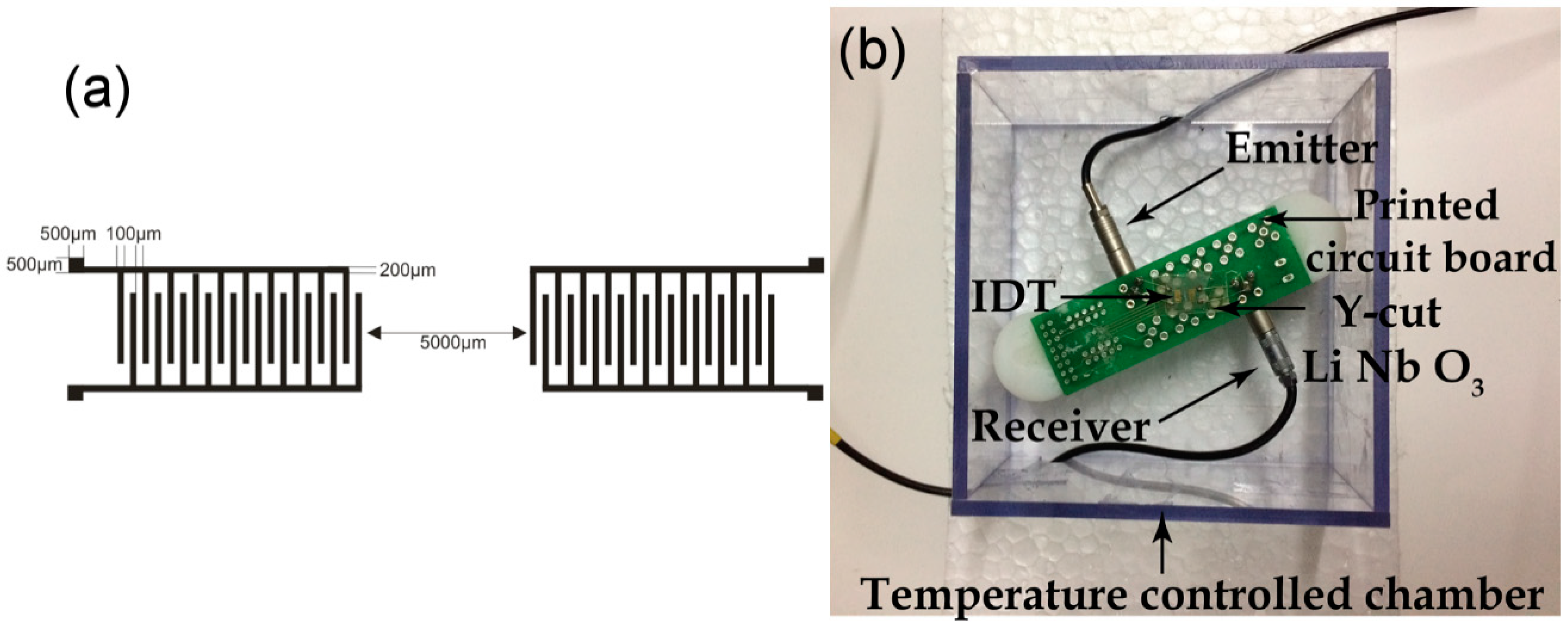
The precursor to the damage is quantified using the nonlocal damage index developed through non-local field theory. To demonstrate the applicability of the proposed formulation, experimental investigation is conducted using a SAW and longitudinal waves in Lithium Niobate crystal, as discussed below. Interdigital electrodes were fabricated on a LiNbO₃ single crystal. The LiNbO₃ crystal was cleaned using acetone, isopropanol, and trichloroethylene for 10 min at a temperature of 60 °C. Then, the wafer was subjected to ultrasonic cleaning treatment for 10 min using de-ionized water. In order to remove the moisture content, the wafer was baked at 120 °C. After cooling the wafer, the photoresist was applied to the surface using the spin coating technique at 4000 rpm for 55 s. Later, the wafer was soft-baked for 10 min at about 125 °C. After soft-baking, the wafer was exposed to UV light (15 mW/cm²) for 2 s. The exposed area of the resist becomes soluble to the developer. This developing procedure continued until the section which was exposed to UV light was completely etched. Then, IDT structures were coated with 0.12 µm gold by thermal evaporation. Then the lift-off technique was adopted to realize the structures. The fabricated individual IDT sensors were bonded to the LiNbO₃ substrate using the ultrasonic wafer bonding method. The schematic diagram of the fabricated IDT and its dimensions is shown in Figure 1a. The experimental setup of for the IDT for SAW propagation in the LiNbO₃ substrate is shown in Figure 1b.

2.2. Defect Detection Using Surface Acoustic Waves

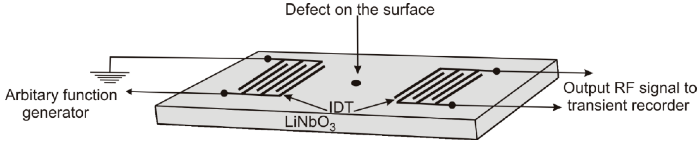
The surface acoustic waves were excited using the IDT, which was fabricated as a SAW sensor on a Y cut LiNbO₃ single crystal. Figure 2, shows the experimental set-up for the excitation and defect detection using IDT. The size of the single electrode was 100 µm in width and 4000 µm in length. The employed resonating frequency of the IDT sensor was 5 MHz and also demonstrated in the next section. The distance between transmitting and receiving IDT sensor was 5 mm and also shown in the Figure 1. The applied voltage across the electrodes produces an electrical field due to the accumulation of charges which alternate in polarity between neighboring electrodes.

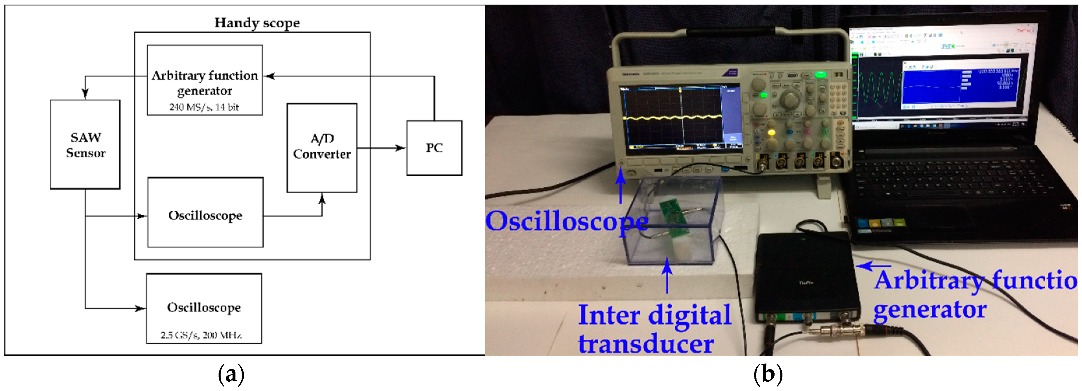
The excitation of compression and expansion movement of phonons perpendicular to the electrodes leads to excitation of surface acoustic waves, also known as Rayleigh waves. The employed arbitrary function generator (AFG) has the capability to generate a linear chirp signal 10 Hz to 25 MHz at the voltage of ±5 volts. A chirp signal was excited using a universal serial bus (USB) driven by the AFG (Handyscope HS3, Tiepie Engineering, The Netherlands). The AFG could generate 240 MS/s, 14-bit, 128 k sample arbitrary signal which could be digitized at a sampling rate of 500 MS/s. The data acquisition was performed using a mixed domain oscilloscope (MDO 3024, Tektronix, Oregon, USA). The data acquisition system has four analog channels with 200 MHz analog bandwidth with a maximum sampling rate of 2.5 GS/s. The record length of the data acquisition system (DAQ) is 10 million points. The entire experiment was carried out in a temperature-controlled chamber and kept over an expanded polystyrene (EPS) foam so that it can suppress low-frequency vibrations and minimize error due to temperature fluctuations. Figure 3a shows the schematic representation of the data acquisition system of the experiments. Figure 3b shows the experimental setup for conducting excitation and detection of SAW’s and longitudinal waves in the LiNbO₃ crystal.

SAW’s have been excited and detected on the reference sample and transient signal was recorded via a transient recorder. Next, a calibrated defect/flaw was created on the surface of the IDT using a high-speed diamond drill of radius 250 µm and 0.2 µm deep, considerable representation of a micro-scale defect in the piezoelectric crystal. The microscale damage of depth 0.2 µm is considered as the precursor to damage. Each experiment of excitation and detection of the ultrasonic wave using IDT was repeated for five times to ensure repeatability. The surface defect/flaw was characterized and imaged by scanning acoustic microscopy (SAM). In the next section, the working principle of SAM has already been described somewhere else [28].

3. Mathematical Derivation

3.1. Nonlocal Kernel and Operator

In this study, we utilize the change in characteristics of surface acoustic wave propagation in the piezoelectric crystal, namely the time of flight (TOF) and its spectral signature, to quantify the precursor to damage. Damage initiation and crack evolution in the material is a multi-scale phenomenon. Interaction of the ultrasonic wave with the micro-crack helps in the detection and quantification of the precursor to damage in the material. The damage diagnosis and prognosis in the piezoelectric ceramics rely on the information of angular dispersion relationship, that is, directional changes in quasi-longitudinal and quasi-shear wave velocity profile. Any perturbation in the directional wave velocity is an important aspect that indicates the “incubation of damage” at the intrinsic length scale. Here, we can now relate the perturbation in wave velocity with the microscale damages/flaws. The study incorporates the nonlocal elastic theory in the framework of micro continuum mechanics and derives the relationship between angular dispersion and nonlocal parameters via Christoffel’s solution [37]. Auld, and Royer and Dieulesaint have explained the mathematical framework of the development of the wave dispersion relationship and angular dispersion [37,38]. The study is efficient in predicting the nonlocal parameter by satisfying the boundary conditions in the first Brillouin zone. Eigenvectors and Eigenvalues from the solution of Christoffel’s equation will be useful to understand the behavioral changes in the solution due to the incorporation of nonlocal parameters [11]. In this work, our aim is to evaluate the change in TOF of the SAW’s in piezoelectric ceramics to quantify the precursor to damage. There are two scenarios to utilize the formulation proposed in nonlocal Christoffel’s solution for quantification of the damage precursor. In the first case, if ab initio dynamics studies are performed on the damaged state of the material and prior information of nonlocal parameters is available then the perturbed velocity profile can be calculated from the nonlocal Christoffel’s solution. In the second case, a dispersion curve is plotted for the varied nonlocal parameters using non-local field theory. The experimental wave velocity and the central frequency are overlaid on the dispersion plots to evaluate suitable nonlocal parameters. The nonlocal parameters will provide a parametric understanding of internal damage occurring even before the crack nucleates. The nonlocal parameter can be used in elegant prognostic theories to predict crack nucleation based on the present damaged state at the intrinsic length scale. The above concept is mathematically formulated and key aspects are discussed below. Patra and Banerjee have employed the similar theoretical model to quantify the precursor to damage in woven carbon composite structure damage under influence of high cycle fatigue loading [39].

Let us assume a position vector of a point in the direct lattice $\overrightarrow{r}={\alpha }_1{\overrightarrow{l}}_1+{\alpha }_2{\overrightarrow{l}}_2+{\alpha }_3{\overrightarrow{l}}_3$ where, ${\overrightarrow{l}}_1,{\overrightarrow{l}}_2$ and ${\overrightarrow{l}}_3$ are the basis vectors of the lattice [40]. The wave potential of a wave propagating through the lattice can be observed only at the lattice points $\overrightarrow{r}$, and the potential can be written as $\varphi =A{e}^{\left\{i\left(k_1{\alpha }_1+k_2{\alpha }_2+k_3{\alpha }_3\right)\right\}}$. The function $\phi$ is periodic in $\overrightarrow{k}=k_1{\overrightarrow{m}}_1+k_2{\overrightarrow{m}}_2+k_3{\overrightarrow{m}}_3$, where $\overrightarrow{k}$ is the wave vector in reciprocal lattice and ${\overrightarrow{m}}_1,{\overrightarrow{m}}_2,{\overrightarrow{m}}_3$ are the basis vectors in reciprocal lattice system. There is an explicit relation between lattice vectors in reciprocal and direct lattices $({\overrightarrow{l}}_i•{\overrightarrow{m}}_k)={\delta }_{ik}$, where, ${\delta }_{ik}$ is the Kronecker $(\delta )$ symbol. Hence, the similar potential is true for a wave vector $\overrightarrow{k^{\prime }}=\overrightarrow{k}+\overrightarrow{g}$, where $\overrightarrow{g}$ is a translation vector ($\overrightarrow{g}={\xi }_1{\overrightarrow{m}}_1+{\xi }_2{\overrightarrow{m}}_2+{\xi }_3{\overrightarrow{m}}_3$) in reciprocal lattice system. There is a specific periodic relationship between the frequency ($\omega$) and $\overrightarrow{k}$ to enforce the lattice scale relationships [40]. This relationship must satisfy the boundary conditions at the boundaries of the Brillouin zones [40], specifically at the boundaries of the first Brillouin zone. The functional relationship presented by Born-Von Kármán from the lattice dynamics study can be further approximated [41]. The approximated atomic dispersion relation can be written as

$$\frac{{\omega }_i(\overrightarrow{k})}{c_i\sqrt{(k_1^2+k_2^2+k_3^2)}}=\frac{1}{\{1+e_0{}^2{\ell }^2(k_1^2+k_2^2+k_3^2)\}}$$

(1)

where, $i$ is indicate waves modes (show, fast shear and longitudinal), ${\epsilon }_{ls}=e_0\ell$ is the intrinsic length scale factor, and $\ell$ is intrinsic length scale such as lattice dimension, granular distance and so on [41]. The operator L can be written as

$$L=(1-{\epsilon }_{ls}^2{\nabla }^2)$$

(2)

where, ${\nabla }^2$ is a Laplace operator in three dimensions. The suitable Kernel function can be written as [42]

$$\kappa (\left|y-x\right|)=\frac{1}{4\pi }\frac{1}{c_p^2-c_s^2}\frac{1}{\left|(y-x)\right|}\left\{\exp \left(-\left|(y-x)\right|/c_p\right)-\exp \left(-\left|(y-x)\right|/c_s\right)\right\}$$

(3)

where, $c_p^2=\frac{{\left(e_0\ell \right)}^2}{2}$

Lazar et al. recommended the use of bi-Helmholtz type operator to circumvent the problem of satisfying the boundary condition [42]. According to Lazar et al. [42], the atomic dispersion relation can be written as

$$\frac{{\omega }_i(\overrightarrow{k})}{c_i\sqrt{(k_1^2+k_2^2+k_3^2)}}=\frac{1}{\{1+e_0{}^2{\ell }^2(k_1^2+k_2^2+k_3^2)+f_0{}^4{\ell }^4{(k_1^2+k_2^2+k_3^2)}^2\}}$$

(4)

where, $f_0\ell$ is the higher order intrinsic length scale factor. The operator which can explicitly catch the dispersion equation at intrinsic length scale has been derived by several researchers [41,43,44] and adopted in the present study. The suitable operator L can be written as

$$L=(1-e_0{}^2{\ell }^2{\nabla }^2)$$

(5)

where, ${\nabla }^2$ is a Laplace operator in three dimensions. The Kernel function can be written as [42]

$$\kappa (\left|y-x\right|)=\frac{1}{4\pi }\frac{1}{c_p^2-c_s^2}\frac{1}{\left|(y-x)\right|}\left\{\exp \left(-\left|(y-x)\right|/c_p\right)-\exp \left(-\left|(y-x)\right|/c_s\right)\right\}$$

(6)

where, $c_{p,s}^2=\frac{{\left(e_0\ell \right)}^2}{2}\left(1\pm \sqrt{1-4\frac{{\left(f_0\ell \right)}^4}{{\left(e_0\ell \right)}^4}}\right)$

3.2. Nonlocal Continuum Theory: Acoustic Waves in Piezoelectric Media

In this section, we derive the angular dispersion relationship of ultrasonic wave propagation in the piezoelectric crystal by incorporating a nonlocal elastic kernel function in Christoffel’s solution. Einstein index notations have been used throughout this paper with indices taking values 1, 2 and 3. Let us consider a body $\mathsf{\Omega }$ with boundary $\mathsf{\Gamma }$. At any point $y$ in $\mathsf{\Omega }$, the constitutive relationship is written as

$${\sigma }_{ij}=C_{ijlm}^E{S}_{lm}-e{p}_{ijr}{E}_r$$

(7)

$$D_r=e{p}_{ijr}{S}_{ij}+{\epsilon }_{rl}^S{E}_l$$

(8)

$\sigma$ denotes the elastic stress tensor, S as elastic strain tensor, the electric field ${\overrightarrow{E}}_r$, ${\overrightarrow{D}}_r$ the electric displacement, $C^E$ the elastic modulus tensor at constant electric field, $ep$ the piezoelectric stress tensor, and ${\epsilon }^S$ the permittivity tensor at constant strain.

Equation (7) represents the experimental stress strain behavior developed in the anisotropic crystal depending on the constraints imposed in the electric field. Equation (8) shows that the resultant stress tensor depends on whether the electric field is allowed to develop in the crystal, if strain S is applied. The piezoelectric effect in the sensor depends on the crystal symmetry. The displacement of microscopic charge in crystal lattice results in the generation of electric displacement in the piezo-electric crystal. The equations of motion can be written as [38].

$$\rho {\ddot{u}}_i(\mathrm{x},\mathrm{t}){\delta }_{il}=\frac{\partial {\sigma }_{ij}}{\partial x_j}$$

(9)

According to the nonlocal elasticity, the stress at a point of interest $x(x_n)$ can be written as

$$t_{ij}(x)={\displaystyle \underset{\mathsf{\Omega }}{\int }{C}_{ijkl}(y)\kappa \left(\left|y-x\right|\right)S_{kl}(y)d\mathsf{\Omega }}$$

(10)

where, $\kappa \left(\left|y-x\right|\right)$ is a nonlocal kernel or nonlocal modulus. Various researchers investigated the suitable use of the nonlocal kernel for specific problem formulation. A list of different types of kernels is presented in the literature [41]. A functional form of nonlocal elasticity kernel is presented by Picu [44] and the potential is developed from a molecular dynamic study. From these past studies, it is concluded that the kernel function can also be considered as the probability density function. The nonlocal kernels have a few specific properties [41]. The integro-differential equation of motion at x can be written as

$${\displaystyle \underset{\mathsf{\Omega }}{\int }\frac{\partial }{\partial x_j}\left(S_{ij}(y)\kappa \left(\left|y-x\right|\right)\right)}d\mathsf{\Omega }(y)+F_i(x)=\rho (x){\ddot{u}}_k{\delta }_{ik}$$

(11)

The above equation can be manipulated in a different way by operating it with the operator L. Thus Equation (11) can be written as

$$C_{ijkl}{\displaystyle \underset{\mathsf{\Omega }}{\int }L\kappa \left(\left|y-x\right|\right)}{S}_{kl,j}(y)d\mathsf{\Omega }(y)+L{F}_i(x)=L\left(\rho (x){\ddot{u}}_k\right){\delta }_{ik}$$

(12)

$$C_{ijkl}{\displaystyle \underset{\mathsf{\Omega }}{\int }\delta \left(\left|y-x\right|\right)}{S}_{kl,j}(y)d\mathsf{\Omega }(y)+L{F}_i(x)=L\left(\rho (x){\ddot{u}}_k\right){\delta }_{ik}$$

(13)

$$C_{ijkl}{S}_{kl,j}(x)-L\left(\rho \left(x\right){\ddot{u}}_k\right){\delta }_{ik}=-L{F}_i(x)$$

(14)

The equation of motion for vibration in anisotropic piezoelectric solid is given as (the dummy index are interchanged, without loss of generality)

$$\rho L({\ddot{u}}_{{}_i}){\delta }_{il}=C_{ijml}^E\frac{{\partial }^2{u}_l}{\partial x_j\partial x_m}-e{p}_{ijr}\frac{\partial E_r}{\partial x_j}$$

(15)

The operator L is given as $L=1-{\epsilon }_{sl}^2{\nabla }^2;{\epsilon }_{sl}=e_{o}l$ is the intrinsic length scale factor.

We are assuming the plane-wave solution in the form $\overrightarrow{u}=u_o{e}^{i\left(\omega t-\overrightarrow{k}\cdot \overrightarrow{x}\right)}$ for displacement and $\varphi ={\varphi }_0{e}^{i\left(\omega t-\overrightarrow{k}\cdot \overrightarrow{x}\right)}$ for scalar electric potential.

The electric field becomes

$$E_l={\left(-\nabla \varphi \right)}_l=i{k}_l{\varphi }_0{e}^{i\left(\omega t-\overrightarrow{k}\cdot \overrightarrow{x}\right)}$$

(16)

that is $\overrightarrow{E}\left|\right|\overrightarrow{k}$. From the absence of free charges, the differential of Equation (8) yields:

$$\frac{\partial D_r}{\partial x_r}=e{p}_{ijr}\frac{\partial S_{ij}}{\partial x_r}+{\epsilon }_{rl}^S\frac{\partial E_l}{\partial x_r}=e{p}_{ijr}\frac{{\partial }^2{u}_i}{\partial x_r\partial x_j}+{\epsilon }_{rl}^S\frac{\partial E_l}{\partial x_r}=0$$

(17)

and, hence the amplitude of scalar potential function is obtained as

$${\varphi }_0=\frac{e{p}_{ijr}{k}_j{k}_r{U}_i}{{\epsilon }_{pq}^S{k}_p{k}_q}$$

(18)

Assuming the plane waves solution, the equation of motion (recall Equation (15)) is simplified as below

$$\rho (1-{\epsilon }_{ls}^2{\nabla }^2){\ddot{u}}_{{}_i}{\delta }_{il}=C_{ijml}^E\frac{{\partial }^2{u}_l}{\partial x_j\partial x_m}-e{p}_{ijr}\frac{\partial E_r}{\partial x_j}$$

(19)

$$\rho {\omega }^2(1-{\epsilon }_{ls}^2{\nabla }^2)u_i{\delta }_{il}=C_{ijml}^E{k}_j{k}_m{u}_l+k_j{k}_m\frac{e{p}_{ijr}{k}_{r}e{p}_{lms}{k}_s}{\left({\epsilon }_{pq}^S{k}_p{k}_q\right)}{u}_l$$

(20)

$$\rho {\omega }^2\left(1+{\epsilon }_{ls}^2\left|k^2\right|\right)u_i{\delta }_{il}=C_{ijlm}^E{k}_j{k}_m{u}_l+k_j{k}_m\frac{e{p}_{ijr}{k}_{r}e{p}_{lms}{k}_s}{\left({\epsilon }_{pq}^S{k}_p{k}_q\right)}{u}_l$$

(21)

The non-trivial solution from Equation (21) is given as

$$C_{ijlm}^E{k}_j{k}_m+k_j{k}_m\frac{e{p}_{ijr}{k}_{r}e{p}_{lms}{k}_s}{\left({\epsilon }_{pq}^S{k}_p{k}_q\right)}-\rho {\omega }^2\left(1+{\epsilon }_{ls}^2\left|k^2\right|\right){\delta }_{il}=0$$

(22)

After dividing by $\rho {\omega }^2$ and introducing the Cartesian components $n_l$ of the unit vector in the direction of k this leads to the modified Christoffel equation given in Equation (23)

$$\frac{\left|k^2\right|}{\rho {\omega }^2}\left[C_{ijlm}^E+\frac{e{p}_{ijr}{n}_{r}e{p}_{lms}{n}_s}{\left({\epsilon }_{pq}^S{n}_p{n}_q\right)}\right]n_j{n}_m-\left(1+{\epsilon }_{ls}^2\left|k^2\right|\right){\delta }_{il}=0$$

(23)

In Equation (23), the square brackets indicate the constitutive matrix considering mechanical and piezoelectric stiffness. In the absence of piezo-electric constants, the equation reduces to the classic Christoffel equation. The right-side term of the square bracket in Equation (23), indicates the piezo-electrically stiffened elastic constants. The stiffened piezo-electric constants are the function of both material properties and direction of propagation.

Let, ${\mathsf{\Gamma }}_{il}=\frac{1}{\rho {\omega }^2}\left[C_{ijlm}^E+\frac{e{p}_{ijr}{n}_{r}e{p}_{lms}{n}_s}{\left({\epsilon }_{pq}^S{n}_p{n}_q\right)}\right]n_j{n}_m$ and $\left|k^2\right|=({\mathrm{k}}_1^2+{\mathrm{k}}_2^2+{\mathrm{k}}_3^2)$

The eigen values analysis of the biharmonic modified Christoffel equation gives

$$\left|{\mathsf{\Gamma }}_{il}-{\delta }_{il}\left(\frac{1}{k^2}+{\epsilon }_{ls}^2\right)\right|=0$$

(24)

The Equation (24) can be written in matrix form as below

$$\left[\begin{array}{ccc}{\mathsf{\Gamma }}_{11}-{\epsilon }_{ls}^2& {\mathsf{\Gamma }}_{12}& {\mathsf{\Gamma }}_{13}\\ {\mathsf{\Gamma }}_{21}& {\mathsf{\Gamma }}_{22}-{\epsilon }_{ls}^2& {\mathsf{\Gamma }}_{23}\\ {\mathsf{\Gamma }}_{31}& {\mathsf{\Gamma }}_{32}& {\mathsf{\Gamma }}_{33}-{\epsilon }_{ls}^2\end{array}\right]-\left[\begin{array}{ccc}\frac{1}{{\left|k\right|}^2}& 0& 0\\ 0& \frac{1}{{\left|k\right|}^2}& 0\\ 0& 0& \frac{1}{{\left|k\right|}^2}\end{array}\right]=0$$

(25)

Finally, Eigen value solution is performed on the following nonlocal Christoffel’s equation

$$\left[\left({\mathsf{\Gamma }}_{ij}-{\epsilon }_{ls}^2{\delta }_{ij}\right)-\frac{1}{{\left|k\right|}^2}{\delta }_{ij}\right]=0$$

(26)

The solution yields solutions for three propagating modes: quasi-longitudinal, fast transversal and slow transversal waves.

The main outcome of the theoretical model is the generation of directional group wave velocity in LiNbO₃ for slow and fast transverse wave velocity considering piezo-electric stiffening. Also, we develop directional group wave velocity for longitudinal wave velocity considering piezo stiffening. The crucial aspect of the theoretical model is an accurate generation of the dispersion relationship of the quasi-slow transversal and quasi-longitudinal wave mode resulting from intrinsic length scale varying from zero to unity. These developed dispersion curves will act as a calibrating chart on which the experimental results will be overlaid to quantify the nonlocal parameters representing a precursor to damage.

4. Analysis of Experimental Results

The surface acoustic and longitudinal waves were excited and detected using the IDT. Fall et al. [45] have studied the generation of broadband SAWs using spatial and temporal chirp method. They argued that the impulse excitation (Dirac delta pulse) produce limited SAWs output amplitude due to piezo-electric breakdown voltage. Fall et al. excited the IDT using temporal chirp excitation corresponding to the frequency and duration of the spatial chirp configuration [45]. In that work, they implemented the chirp excitation methods for a wide range from 20 MHz–125 MHz. The excitation of IDT with chirp provides a rapid, accurate estimation of phase velocity and helps in material characterization.

For high frequency (>100 MHz) applications, the IDT is designed for the specific center frequency. At high frequencies, the losses due to attenuation and scattering along the comb of IDT are larger. In high frequency and broadband chirp excitation the IDT will distribute the energy throughout the frequency spectra, resulting in greater energy losses. The resonating frequency ($f_o$) response of the simple transducer with $N$ pair of fingers is deduced from the impulse response. A frequency domain response of the impulse excitation has a broadband spectrum. A pulse is usually applied to the electrode having a short duration compared to the time associated with the Rayleigh waves to pass between two finger length [39]. As the electric field is reversed at each interval between figures, the transmitted signal has a spatial period of 2d. The time duration of response is $\mathsf{\Theta }=\frac{2dN}{V_R}=\frac{N}{f_0}$. On the other hand, at low frequency (<10 MHz) application, the resonating frequency is commonly determined using broadband chirp excitation rather than the impulse response.

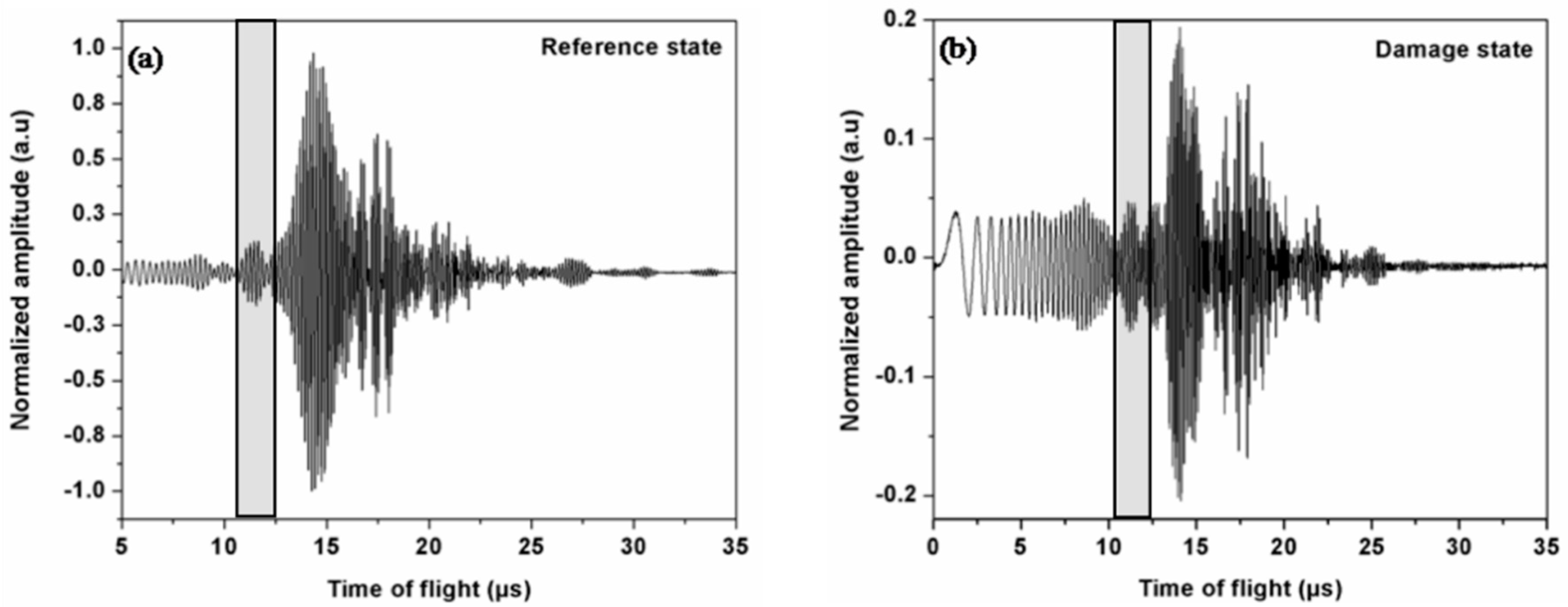
The low resonant frequency IDT was fabricated for excitation and detection of the guided wave for detection of aberration, abnormality and surface cracks. For nondestructive evaluation applications, the resonating frequency of IDT rarely exceeds 20 MHz. In order to determine the resonating frequency of the referenced sensor, the IDT was excited using chirp signals and we evaluated its frequency response. A linear chirp used for excitation of ultrasonic wave is given by $x(t)=A\sin \left(2\pi ft\right)$ of sinusoidal frequency, $f$. Considering that the active length of IDT is 4 mm, the temporal signal duration $\left(T_c\right)$ is 1.12 μs. The instantaneous frequency is calculated as $f=\left(f_c-\frac{\Delta f}{2}\right)+\frac{\Delta f}{2T_c}t$. Here $f_c$ is the average frequency and $\Delta f$ is the difference of lower and upper limit of frequency spectrum as obtained from chirp excitation. Initially, the chirp excitation frequency was 10 Hz–20 MHz. Based on the Fourier spectra, it was observed that the dominant mode exists in the frequency range of 4 MHz–7 MHz. Therefore, in the damage state, the frequency of excitation was narrowed down between 1 MHz–10 MHz. The range of excitation frequency was quite large, to account for dispersion and scattering of the wave due to surface cracks. The IDT was excited using linear chirp and the received transient signal of the SAW for the reference sensor is shown in Figure 4a. The signal is normalized to unity using the maximum amplitude of 125 millivolts of the reference state. Similarly, the transient signal for the defective sensors excited using linear chirp signal is shown in Figure 4b. There is a dramatic change in normalized amplitude of the signal from 1 to 0.2 (arbitrary units) corresponding to reference state and damage state, respectively. In Figure 4 and Figure 5, the shaded section indicates the window used for evaluating the Fourier transform of the first arrival wave packet.

Figure 5 shows the frequency spectrum of the first arrival wave packet for the reference and damaged sensor. For the reference sensors (black), the significant spectral peak was observed at 5.8 MHz (refer to Figure 5). For the damaged sample, the peak central frequency (grey) is at 5.1 MHz. The chirp signal helps in exciting the natural frequency of health as well as crack sensors, irrespective of the IDT design.

We observed that the resonating frequency of the damage sensors shifts towards the left with respect to the reference sensors. The wavelength of the guided wave is in close proximity to the thickness of the piezoelectric sensor. During the propagation, the wave interacts with the thickness and the energy content of the elastic wave is dispersed throughout the thickness and length of the media. The energy of the guided waves is scattered, in the presence of the surface anomalies such as crack, inter-laminar debonding, and delamination. The scattering phenomena are complex to understand in the absence of full wave-field imaging. The scattering further influences the dispersion of elastic waves, which is evident in the frequency domain of the signal (Figure 5). Based on the experimental results it is evident that there exists a damage (preferably on the surface) which is manifested through the difference in TOF and the shift in the frequency spectrum acquired through IDT.

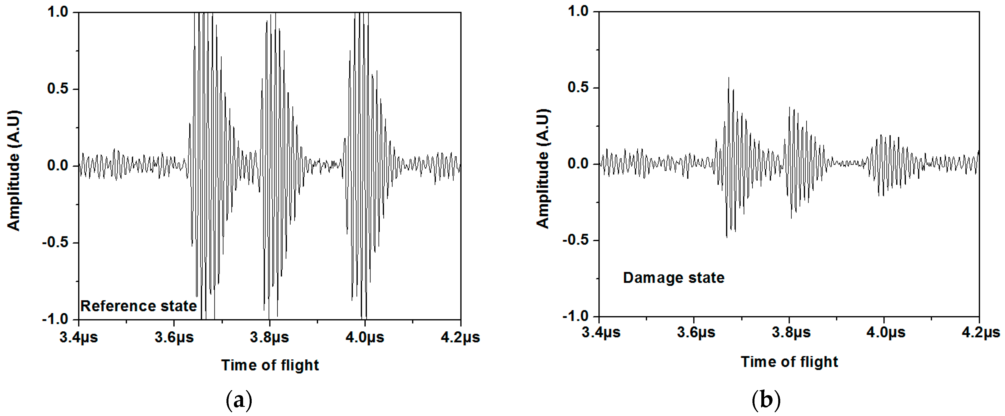
Figure 6 shows the time domain signal for the reference and damage state acquired using SAM at 100 MHz. The time domain signal in the reference state (Figure 6a) is normalized to the unit using the peak reference voltage of 220 millivolts. Similarly, the time domain signal in the damage state (Figure 6b) is normalized with respect to peak amplitude in the reference state. Figure 6a,b show three distinct arrival peaks due to excitation of longitudinal waves in the Y cut LiNbO₃. The first and second arrival peak corresponds to the reflection of longitudinal waves from the top and bottom surface of the crystal. The third arrival peak is the surface reflection of longitudinal waves from the printed circuit board (PCB). It is observed that the peak amplitude is dramatically reduced from unity to half, corresponding to reference state to damage state, respectively. Reduction in the amplitude of the reflected signal is due to the surface damage. The longitudinal waves are dispersed due to surface detection, as visible from the time domain signal (Figure 6b and Figure 7b). To accurately quantify the frequency content of reference and damage state, we performed a Fourier transform on Figure 6a,b.

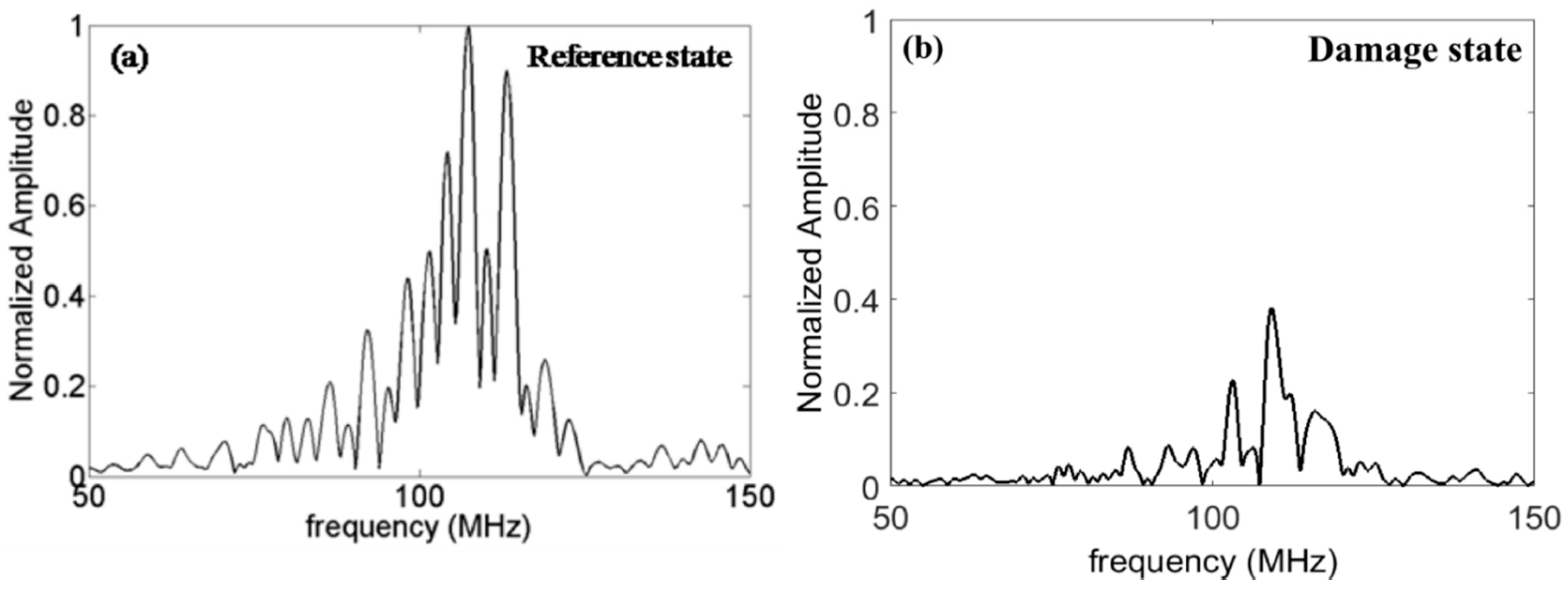
The normalized frequency domain signal in the reference state shows two distinct peak amplitudes at 107 MHz and 113 MHz at a unit amplitude and 0.88 (arbitrary units) amplitude, respectively (Figure 7a). Due to damage, the energy of the signal is dispersed, scattered, and attenuated, resulting in a reduction of peak amplitude to 0.38. For the damage signal, the mode one peak amplitude is reduced to 0.22 at a frequency of 103 MHz and mode two peak amplitude is reduced to 0.38 at a frequency of 109 MHz, respectively.

In conventional methods, these observational changes in frequencies have been identified as a measure of damage. However, the consistent and reliable quantification of damage is rather difficult. Several experimental investigations have been conducted to explore the utility of guided waves for crack detection. The pitch-catch active sensing method has been employed for crack detection in aerospace structures using guided ultrasonic waves [46]. Shelke et al., 2011, have studied the metamorphosis of the bulk wave to guided waves and its interaction with surface defects [34]. The scattering of the guided waves due to cracks, defects and surface anomalies has been studied using a scanning laser vibrometer. The wave field imaging provides dispersion and scattering behavior of ultrasonic waves in the spatial-temporal and wave-number-frequency domain [47,48]. The above techniques are based on the complete wave field imaging, which provides detailed information regarding propagation of guided wave in anisotropic solids. However, little literature is available on guided wave propagation in anisotropic piezoelectric crystals. Also, the above technique is computationally expensive and time-consuming. The particle utility of the wave field imaging technique is limited in the laboratory environment. There is no systematic understanding and quantification process that relates this signal to the material physics. It is imperative that the quantification of the magnitude of damage could not be determined alone from the experimental results by tracking changes in amplitude and shift in frequency of the signal.

Therefore, we formulated a non-local elastic wave propagation theory to relate the changes in the nonlocal material physics and quantify them reliably and consistently. We formulate nonlocal parameters, which are indicative of micro-scale aberration on surface and subsurface defects in the piezoelectric crystal.

5. Results and Discussions

In this section, we combine the understanding from Section 2, Section 3 and Section 4. Directional group velocities are calculated for Lithium Niobate piezoelectric crystal considering piezoelectric stiffening using Equation (26) [37]. The constitutive material properties of LiNbO₃ is given in

Table 1. Acoustic physical constant of LiNbO₃ of single crystal.

Elastic Constant (×1011 N/m2)			Piezoelectric Constant (C/m2)
$C_{11}^E$	1.9886	$C_{15}$	3.655
$C_{12}^E$	0.5467	$C_{22}$	2.407
$C_{13}^E$	0.6799	$C_{31}$	0.328
$C_{14}^E$	0.0783	$C_{33}$	1.894
$C_{33}^E$	2.3418	Dielectric constant
$C_{44}^E$	0.5985	${\epsilon }_{11}^S/{\epsilon }_O$	44.9
$C_{66}^E$	0.7209	${\epsilon }_{33}^S/{\epsilon }_O$	26.7

(Kushibiki et al., 1999) [49].

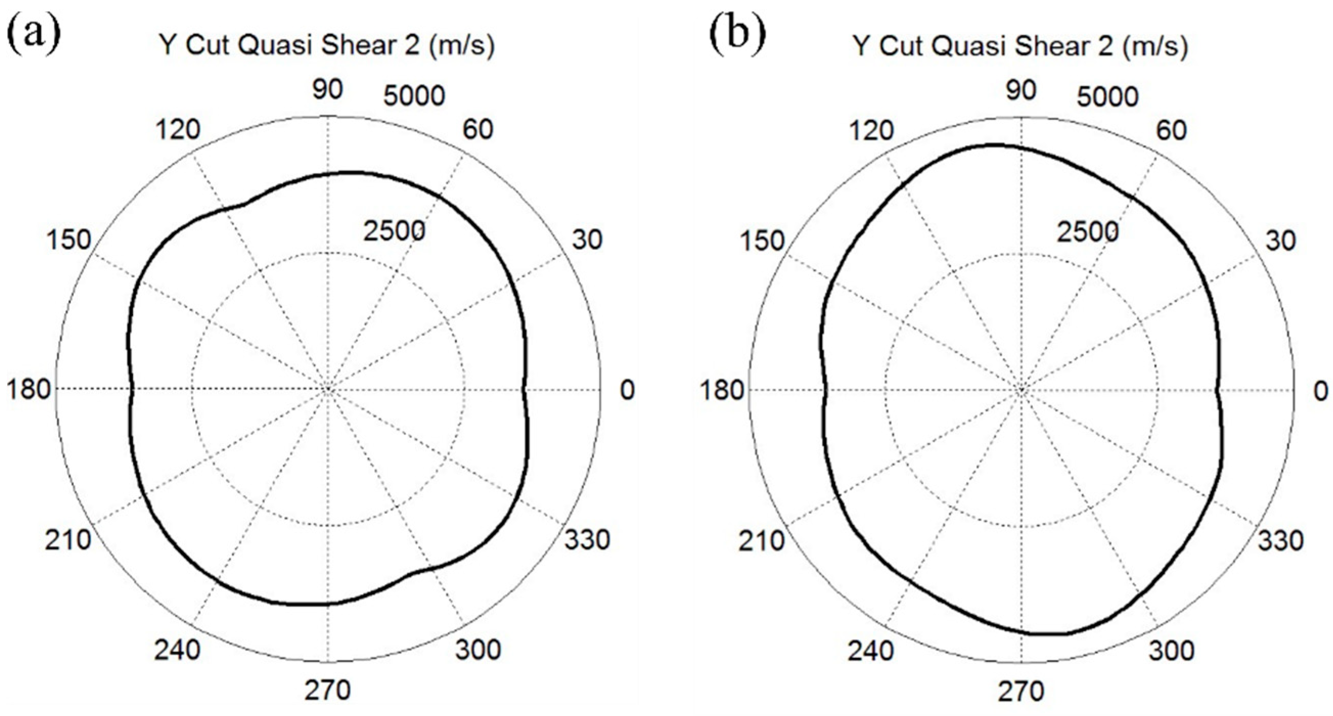
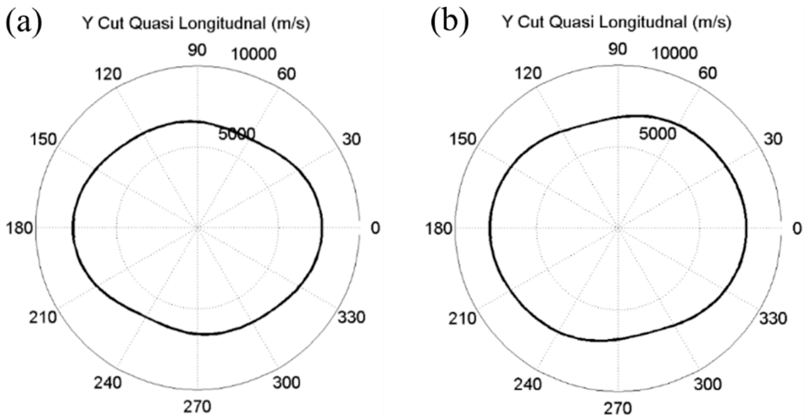
Figure 8a, Figure 9a and Figure 10a show directional slow transversal, fast transversal and longitudinal group wave velocity for LiNbO₃ without piezo stiffening. Similarly,Figure 8b, Figure 9b and Figure 10b show directional slow transversal, fast transversal and longitudinal group wave velocity for LiNbO₃ with piezo stiffening. The angular dispersions shown in Figure 8, Figure 9 and Figure 10 are calculated for a nominal elastic and piezoelectric properties at zero intrinsic length scale parameter ${\epsilon }_{ls}=0$ and referred to as undamaged or reference state. At zero-degree orientation of wave propagation, the group wave velocity for a slow transversal wave in non-piezo stiffened and piezo stiffened materials are 3571 m/s and 3592 m/s, respectively. However, for longitudinal waves, the computed group velocities are 7696 m/s and 7873 m/s in non-piezo and piezo stiffened materials. We assume that any changes in the group wave velocity of the transversal wave mode are due to the surface damage, which is the manifestation of the perturbation in elastic material constants alone but independent of piezoelectric constants. The same cannot be argued for the longitudinal wave velocity, as piezo stiffening plays a significant role in governing the group wave velocity. Therefore, any alteration in group wave velocity of the longitudinal wave is due to a combined effect from the degradation of mechanical and piezoelectric constants.

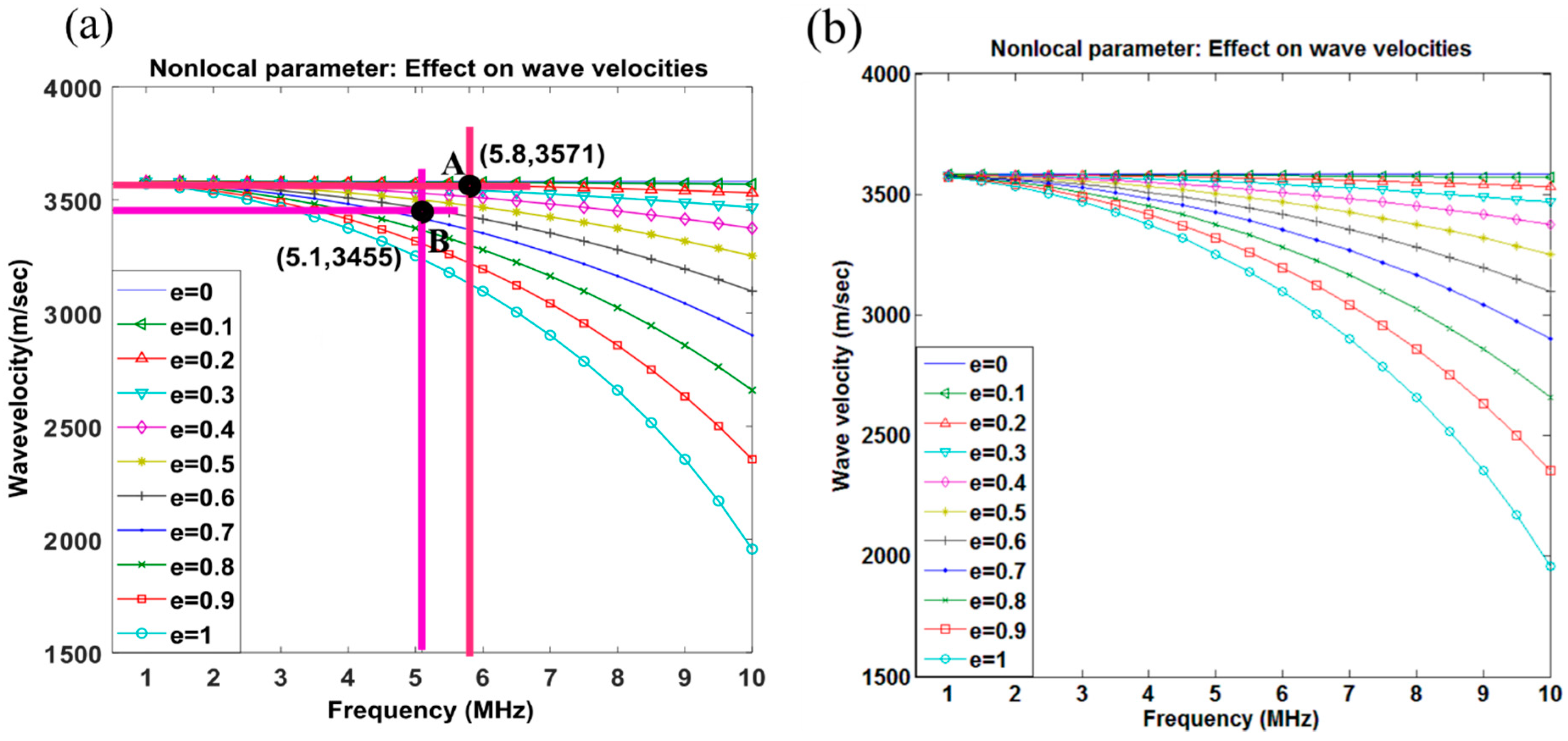
In order to quantify the relative magnitude of the damage on the sample, dispersion relationship (group velocity vs frequency) are plotted for LiNbO₃ for non-piezo and piezoelectric stiffened (refer Section 2) specimens. Figure 11 and Figure 12 represent the dispersion relation of the LiNbO₃ considering intrinsic length scale nonlocal parameter ${\epsilon }_{ls}$ ranging from 0 to 1, where ${\epsilon }_{ls}$ = 0 is an undamaged state and ${\epsilon }_{ls}$ = 1 is relative complete damage state. Figure 11a,b and Figure 12a,b show the dispersion relationship considering piezo and non-piezo stiffening for slow transversal and longitudinal waves velocity, respectively. The dispersion relationship shows lowering in group velocity with an increase in frequency for the given wave mode. Also, the group wave velocity decreases with an increase in nonlocal parameter magnitude. It is observed that the surface and subsurface defects will cause scattering, reflection, and attenuation of guided waves leading to change in time of flight (TOF).

6. A Damage Quantification Based on SAW

The changes in time of flight of the SAW due to perturbation in surface material properties were determined using cross-correlation technique. Shelke et al. have shown that such small differences in TOF (>10 ns) can be obtained using cross-correlation where the sampling rate of the signal is significantly high [50]. Referring to the experimental results (Section 4), the TOF of the first arrival is determined using the cross-correlation technique applied to the time history obtained from the undamaged and damaged sample. The cross-correlation technique was employed to determine the first arrival of the time of flight. The excitation signal was selected as the reference signal. The reference signal was cross-correlated with the first arrival time of the flight signal. We correlated the leading edge of the reference signal with the leading wave packet of the received signal. The maximum cross-correlation of the reference signal with the received signal demarks first arrival TOF. Therefore, the dispersive nature of the guided wave is not considered during the determination of the first arrival. The active time duration of excitation was 1.12 μs and the total duration of the received signal is 30 μs. Therefore, sufficient time difference was presence for avoiding the interaction of input chirp wave with the total duration of flight of the guided wave. Our intention was to determine the first arrival of time of flight of guided waves and thus the time of the flight of the multimodal signal are not considered in the analysis. Based on the cross-correlation technique, the difference in the SAWs first arrival in TOF of the damaged and undamaged sample was determined to be 47 ns (refer Figure 5a,b). Such small differences in TOF can only be obtained if the sampling rate of the signal is significantly high. The group velocity of the SAW wave mode in the undamaged specimen is 3571 m/s and in the damaged specimen is 3455 m/s. We assume that the path length between the transmitting and receiving IDT was not changed in the presence of microcrack of depth 0.2 micron. The microscale damage in the path of SAW causes scattering and attenuation of waves. The surface micro defect influences the time of flight of SAW and caused internal multiple reflections. It is usually difficult to quantify the multiple paths of scattering and reflection of SAW in presence of defects. Shelke et al. have demonstrated that the changes in time of flight (TOF) are attributed to the scattering, reflection, and attenuation of guided waves in the presence of surface and subsurface defects [11].

Based on the changes in TOF, we concluded that the surface damage exists on the sample. It can be seen in Figure 7 that the central frequency for undamaged and damage state is 5.8 MHz and 5.1 MHz respectively. Due to changes in TOF, the speed of transversal wave velocity in reference state and damage state is 3571 m/s and 3455 m/s, respectively. In Figure 11, a point “A” is marked having abscissa and ordinate as 5.8 MHz and 3571 m/s respectively. The point “A” overlay on the nonlocal line has the nonlocal damage parameter as 0.1. Similarly, in the Figure 11, a point “B” is marked having an abscissa and ordinate as 5.1 MHz and 3455 m/s. Point “B” lies on the nonlocal damage parameter line of 0.7. Therefore, the difference of the two nonlocal intrinsic length scale parameters is $\Delta \epsilon =0.6$. This concept of change in frequency and velocity of transversal wave is used to quantify the nonlocal intrinsic length scale parameter. The value of the intrinsic parameter indicates the magnitude of damage in the sensors that indicate the precursor to damage.

Damage Quantification Based on Longitudinal Waves

From numerical results, the speed of sound in non-piezo stiffened and piezo stiffened specimens were determined to be 7696 m/s and 7873 m/s, respectively. Referring to Figure 6a, the experimental speed of the longitudinal wave in reference state was determined to be 7692 m/s. Similarly, the experimental speed of the longitudinal wave in damage state was determined to be 6666 m/s. The normalized frequency domain signal in the reference state shows a distinct peak amplitude at 107 MHz at unit amplitude (Figure 7a). For the damaged state, the peak amplitude is reduced to 0.38 and the frequency is shifted to 109 MHz.

A similar procedure is adapted to quantify the nonlocal intrinsic length scale parameter using longitudinal waves. Due to changes in TOF, the speed of longitudinal wave velocity in reference state and damage state is 7692 m/s and 6666 m/s, respectively. In Figure 12, a point “A” is marked having abscissa and ordinate as 107 MHz and 7692 m/s respectively. The point “A” overlay on the nonlocal line has a nonlocal damage parameter of 0.4. Similarly, in Figure 12, a point “B” is marked having an abscissa and ordinate as 109 MHz and 6666 m/s. The point “B” lies on the nonlocal damage parameter line between 0.9 and 1.0. The nonlocal line index was interpolated and the has an index of 0.96. The final value of nonlocal intrinsic length scale parameter is $\Delta \epsilon =0.56$.

The results are summarized in

Table 2. Summary of the numerical and experimental results.

Waves Type and State		Experimental		Theory		Nonlocal Parameter
		Frequency (MHz)	Velocity (m/s)	Non Piezo Stiffened (m/s)	Piezo-Stiffened (m/s)	Piezo-Stiffened	Non Piezo-Stiffened
Longitudinal	Reference	107	7692 ± 4	7696	7873	$0.6$	$0.8$
	Damage	109	6666 ± 10
Transversal	Reference	5.8	3571 ± 8	3564	3592	$0.6$	$0.6$
	Damage	5.1	3455 ± 12

showing numerical and experimental speed of sound for piezo and non-piezo stiffening. The Table 2 also summarized information of shift in frequency content for reference state and damage state which are used to quantify the nonlocal damage parameter.

7. Conclusions

The outcome of this study is the quantification of precursors to damage using hybrid nonlocal micro-continuum mechanics in the piezoelectric anisotropic sensors. The incubation of damage at the micro scale acts as a precursor to the macro-scale effect, which is an indicator for prognosis of the damage. In this study, a micro-scale surface crack of 0.2 µm depth is quantified using the proposed formulation. An intrinsic length scale parameter obtained from nonlocal micro-continuum mechanics is evaluated and used as an indicator of precursors to damage. The experimental investigations were performed to detect damage in a LiNbO₃ crystal using IDT sensors and scanning acoustic microscopy. The manifestation of surface flaws upon characteristic changes in SAWs and longitudinal bulk wave propagations were investigated for damage detection. The changes in TOF and frequency content of the surface acoustic waves and bulk waves are studied for the detection and quantification of the damage. In order to quantify the manifestation of surface defects on the waves characteristic, the explicit expressions of the wave dispersion in anisotropic piezoelectric sensors are derived. The dispersion relationship for the anisotropic solid is derived using Christoffel equations, which incorporate the effect of intrinsic length scale parameters at micro scale.

Based on the nonlocal elastic kernel theory, angular dispersion relationships are plotted for longitudinal, fast and slow transversal wave velocities considering the piezo stiffening in piezoelectric crystal. The study evaluates experimental changes in speed of sound and frequency shift of SAWs and longitudinal waves and is overlaid on theoretical dispersion curves. The reference state of the piezoelectric sensors is considered to have intrinsic length scale parameter e = 0. The damage initiation and evolution in sensors is quantified using the nonlocal parameter with respect to the reference state. All of the results presented in this study are summarized in Table 1. The speed of the longitudinal and transversal waves in the reference state (e = 0) is evaluated as 7692 m/s and 3571 m/s, respectively. Due to the presence of the micro-crack on the surface of the LiNbO₃ crystal, the speed of longitudinal and transversal waves is determined as 6666 m/s and 3455 m/s, respectively. Instead of determining the exact depth of the micro-crack, we envisage quantifying the magnitude of severity of the damage using the nonlocal damage parameter. The influence of the severity of damage on longitudinal waves is quantified using nonlocal parameter $\Delta {\epsilon }_{ls}^{piezo}=0.6$. Similarly, the nonlocal parameter of $\Delta {\epsilon }_{ls}^{piezo}=0.6$ was quantified depicting the influence of damage on transversal wave propagation. The relative change in magnitude of nonlocal parameter reflects the manifestation of severity of damage.

References

- Ito, H.; Takyu, C.; Inaba, H. Fabrication of periodic domain grating in LiNbO3 by electron-beam writing for application of nonlinear optical processes. Electron. Lett. 1991, 27, 1221–1222. [Google Scholar] [CrossRef]
- Fujimura, M.; Kmtaka, K.; Suhara, T.; Nishihara, H. LiNbO3 waveguide quasiphase-matching second harmonic generation deviceswith ferroelectric-domain-inverted gratings formed by electron-beam scanning. J. Light. Technol. 1993, 11, 1360–1368. [Google Scholar] [CrossRef]
- Roshchupkin, D.V.; Fournier, T.; Brunel, M.; Plotitsyna, O.A.; Sorokin, N.G. Scanning electron-microscopy observation of excitation of the surface acoustic-waves by the regular domain-structures in the LiNbO3 crystals. Appl. Phys. Lett. 1992, 60, 2330–2331. [Google Scholar] [CrossRef]
- Lu, Y.Q.; Wan, Z.L.; Wang, Q.; Xi, Y.X.; Ming, N.B. Electro-optic effect of periodically poled optical superlattice LiNbO3 and its applications. Appl. Phys. Lett. 2000, 77, 3719–3721. [Google Scholar] [CrossRef]
- Smith, R.; Welsh, F. Temperature dependence of the elastic, piezoelectric, and dielectric constants of lithium tantalate and lithium niobate. J. Appl. Phys. 1971, 42, 2219–2230. [Google Scholar] [CrossRef]
- Lewis, M.F. High-frequency acoustic plate mode device employing interdigital transducers. Electron. Lett. 1981, 17, 819–821. [Google Scholar] [CrossRef]
- Rocha-Gaso, M.-I.; March-Iborra, C.; Montoya-Baides, Á.; Arnau-Vives, A. Surface generated acoustic wave biosensors for the detection of pathogens: A review. Sensors 2009, 9, 5740–5769. [Google Scholar] [CrossRef] [PubMed]
- Dow, A.B.A.; Ahmed, A.; Bittner, A.; Popov, C.; Schmid, U.; Kherani, N.P. 15 GHz saw nano-transducers using ultrananocrystalline diamond/aln thin films. In Proceedings of the 2012 IEEE International Ultrasonics Symposium, Dresden, Germany, 7–10 October 2012; pp. 968–971. [Google Scholar]
- Farrar, C.R.; Worden, K. An introduction to structural health monitoring. Philos. Trans. R. Soc. A 2007, 365, 303–315. [Google Scholar] [CrossRef] [PubMed] [Green Version]
- Kundu, T. Ultrasonic Nondestructive Evaluation: Engineering and Biological Material Characterization; CRC Press: Boca Raton, FL, USA, 2003. [Google Scholar]
- Shelke, A.; Kundu, T.; Amjad, U.; Hahn, K.; Grill, W. Mode-selective excitation and detection of ultrasonic guided waves for delamination detection in laminated aluminum plates. IEEE Trans. Ultrason. Ferroelect. Freq. Control. 2011, 58, 567–577. [Google Scholar] [CrossRef] [PubMed]
- Habib, A.; Shelke, A.; Pluta, M.; Pietsch, U.; Kundu, T.; Grill, W. Scattering and attenuation of surface acoustic waves and surface skimming longitudinal polarized bulk waves imaged by coulomb coupling. AIP Conf. Proc. 2012, 1433, 247–250. [Google Scholar] [CrossRef]
- Habib, A.; Ahmad, A.; Wagle, S.; Ahluwalia, B.S.; Melandsø, F.; Tiwari, A.K.; Mehta, D.S. Quantitative phase measurement for the damage detection in piezoelectric crystal using angularly placed multiple inter digital transducers. In Proceedings of the 2016 IEEE International Ultrasonics Symposium (IUS), Tours, France, 18–21 September 2016; pp. 1–4. [Google Scholar]
- Pamwani, L.; Habib, A.; Melandsø, F.; Ahluwalia, B.S.; Shelke, A. Single-input and multiple-output surface acoustic wave sensing for damage quantification in piezoelectric sensors. Sensors 2018, 18, 2017. [Google Scholar] [CrossRef] [PubMed]
- Stoney, R.; Geraghty, D.; O’Donnell, G.E. Characterization of differentially measured strain using passive wireless surface acoustic wave (saw) strain sensors. IEEE Sens. J. 2014, 14, 722–728. [Google Scholar] [CrossRef]
- Humphries, J.R.; Malocha, D.C. Wireless saw strain sensor using orthogonal frequency coding. IEEE Sens. J. 2015, 15, 5527–5534. [Google Scholar] [CrossRef]
- Hara, M.; Mitsui, M.; Sano, K.; Nagasawa, S.; Kuwano, H. Experimental study of highly sensitive sensor using a surface acoustic wave resonator for wireless strain detection. Jpn. J. Appl. Phys. 2012, 51, 07GC23. [Google Scholar] [CrossRef]
- Alshits, V.; Darinskii, A.; Lothe, J. On the existence of surface waves in half-infinite anisotropic elastic media with piezoelectric and piezomagnetic properties. Wave Motion 1992, 16, 265–283. [Google Scholar] [CrossRef]
- Anderson, O.; Schreiber, E.; Soga, N. Elastic Constants and Their Measurements; McGraw-Hill: New York, NY, USA, 1973. [Google Scholar]
- Mizuki, J.; Chen, Y.; Ho, K.-M.; Stassis, C. Phonon dispersion curves of bcc Ba. Phys. Rev. B 1985, 32, 666. [Google Scholar] [CrossRef]
- Hayes, W.; Loudon, R. Light Scattering by Crystals; Wiley: New York, NY, USA, 1978. [Google Scholar]
- Papadakis, E.P. Ultrasonic velocity and attenuation: Measurement methods with scientific and industrial applications. In Physical Acoustics; Elsevier: New York, NY, USA, 1976; Volume 12, pp. 277–374. [Google Scholar]
- Melcher, R.; Mason, W.; Thurston, R. Physical Acoustics Vol. XII; Academic Press: New York, NY, USA, 1976. [Google Scholar]
- Northrop, G.; Wolfe, J. Nonequilibrium phonon dynamics. In Nato Asi Series B; Plenum Press: New York, NY, USA, 1985; Volume 124. [Google Scholar]
- Briggs, A.; Kolosov, O. Acoustic Microscopy; Oxford University Press: Oxford, UK, 2010; Volume 67. [Google Scholar]
- Lemons, R.; Quate, C. Acoustic microscope—Scanning version. Appl. Phys. Lett. 1974, 24, 163–165. [Google Scholar] [CrossRef]
- Grill, W.; Hillmann, K.; Würz, K.U.; Wesner, J. Scanning ultrasonic microscopy with phase contrast. In Advances in Acoustic Microscopy; Springer: Berlin, Germany, 1996; pp. 167–218. [Google Scholar]
- Habib, A.; Shelke, A.; Vogel, M.; Pietsch, U.; Jiang, X.; Kundu, T. Mechanical characterization of sintered piezo-electric ceramic material using scanning acoustic microscope. Ultrasonics 2012, 52, 989–995. [Google Scholar] [CrossRef] [PubMed]
- Habib, A.; Shelke, A.; Vogel, M.; Brand, S.; Jiang, X.; Pietsch, U.; Banerjee, S.; Kundu, T. Quantitative ultrasonic characterization of c-axis oriented polycrystalline aln thin film for smart device application. Acta Acust. United Acust. 2015, 101, 675–683. [Google Scholar] [CrossRef]
- Wagle, S.; Habib, A.; Melandsø, F. Ultrasonic measurements of surface defects on flexible circuits using high-frequency focused polymer transducers. Jpn. J. Appl. Phys. 2017, 56, 07JC05. [Google Scholar] [CrossRef] [Green Version]
- Veidt, M.; Sachse, W. Ultrasonic point-source/point-receiver measurements in thin specimensa. J. Acoust. Soc. Am. 1994, 96, 2318–2326. [Google Scholar] [CrossRef]
- Habib, A.; Evgeny, T.; von Buttlar, M.; Pluta, M.; Schmachtl, M.; Wannemacher, R.; Grill, W. Acoustic holography of piezoelectric materials by coulomb excitation. In Proceedings of the Health Monitoring of Structural and Biological Systems, San Diego, CA, USA, 26 February–2 March 2006; p. 61771A. [Google Scholar]
- Habib, A.; Shelke, A.; Pluta, M.; Kundu, T.; Pietsch, U.; Grill, W. Imaging of acoustic waves in piezoelectric ceramics by coulomb coupling. Jpn. J. Appl. Phys. 2012, 51, 07GB05. [Google Scholar] [CrossRef]
- Shelke, A.; Habib, A.; Amjad, U.; Pluta, M.; Kundu, T.; Pietsch, U.; Grill, W. Metamorphosis of bulk waves to lamb waves in anisotropic piezoelectric crystals. In Proceedings of the Health Monitoring of Structural and Biological Systems, San Diego, CA, USA, 6–10 March 2011; p. 798415. [Google Scholar]
- Habib, A.; Amjad, U.; Pluta, M.; Pietsch, U.; Grill, W. Surface acoustic wave generation and detection by coulomb excitation. In Proceedings of the Health Monitoring of Structural and Biological Systems, San Diego, CA, USA, 7–11 March 2010; p. 6501T. [Google Scholar]
- Habtour, E.; Cole, D.P.; Riddick, J.C.; Weiss, V.; Robeson, M.; Sridharan, R.; Dasgupta, A. Detection of fatigue damage precursor using a nonlinear vibration approach. Struct. Control. Health Monit. 2016, 23, 1442–1463. [Google Scholar] [CrossRef]
- Auld, B.A. Acoustic Fields and Waves in Solids; John Wiley & Sons: Hoboken, NJ, USA, 1973; Volume 1. [Google Scholar]
- Royer, D.; Dieulesaint, E. Elastic Waves in Solids II: Generation, Acousto-Optic Interaction, Applications; Springer Science & Business Media: Berlin, Germany, 1999. [Google Scholar]
- Patra, S.; Banerjee, S. Material state awareness for composites part II: Precursor damage analysis and quantification of degraded material properties using quantitative ultrasonic image correlation (quic). Materials 2017, 10, 1444. [Google Scholar] [CrossRef] [PubMed]
- Brillouin, L. Wave Propagation in Periodic Structures: Electric Filters and Crystal Lattices; Dover Publications: New York, NY, USA, 2003. [Google Scholar]
- Eringen, A.C. On differential equations of nonlocal elasticity and solution of skew dislocation and surface waves. J. Appl. Phys. 1983, 54, 4703–4710. [Google Scholar] [CrossRef]
- Lazar, M.; Maugin, G.A.; Aifantis, E.C. On a theory of nonlocal elasticity of bi-helmholtz type and some applications. Int. J. Solids Struct. 2006, 43, 1404–1421. [Google Scholar] [CrossRef]
- Silling, S.A. Reformulation of elasticity theory for discontinuities and long-range forces. J. Mech. Phys. Solids 2000, 48, 175–209. [Google Scholar] [CrossRef] [Green Version]
- Picu, R. On the functional form of non-local elasticity kernels. J. Mech. Phys. Solids. 2002, 50, 1923–1939. [Google Scholar] [CrossRef]
- Fall, D.; Duquennoy, M.; Ouaftouh, M.; Smagin, N.; Piwakowski, B.; Jenot, F. Generation of broadband surface acoustic waves using a dual temporal-spatial chirp method. J. Acoust. Soc. Am. 2017, 142, EL108–EL112. [Google Scholar] [CrossRef] [PubMed]
- Ihn, J.-B.; Chang, F.-K. Pitch-catch active sensing methods in structural health monitoring for aircraft structures. Struct. Health Monit. 2008, 7, 5–19. [Google Scholar] [CrossRef]
- Michaels, T.E.; Michaels, J.E.; Ruzzene, M. Frequency–wavenumber domain analysis of guided wavefields. Ultrasonics 2011, 51, 452–466. [Google Scholar] [CrossRef] [PubMed]
- Mesnil, O.; Leckey, C.A.; Ruzzene, M. Instantaneous and local wavenumber estimations for damage quantification in composites. Struct. Health Monit. 2015, 14, 193–204. [Google Scholar] [CrossRef]
- Kushibiki, J.-I.; Takanaga, I.; Arakawa, M.; Sannomiya, T. Accurate measurements of the acoustical physical constants of LiNbO/sub 3/and LiTao/sub 3/single crystals. IEEE Trans. Ultrason. Ferroelectr. Freq. Control 1999, 46, 1315–1323. [Google Scholar] [CrossRef] [PubMed]
- Shelke, A.; Banerjee, S.; Kundu, T.; Amjad, U.; Grill, W. Multi-scale damage state estimation in composites using nonlocal elastic kernel: An experimental validation. Int. J. Solids Struct. 2011, 48, 1219–1228. [Google Scholar] [CrossRef]
Figure 1.
(a) Schematic representation of the fabricated interdigital transducers (IDT) marked with all the dimensions and, (b) Experimental setup of the fabricated IDT is a temperature-controlled chamber for excitation and detection of S surface acoustic waves (SAWs) and longitudinal waves.
Figure 2.
A schematic representation of the IDT experiments for damage detection in Lithium Niobate (LiNbO3) crystal.
Figure 3.
(a) Schematic representation for generation of SAWs and longitudinal waves using IDT sensors and (b) experimental setup for conducting excitation and detection of SAWs using IDT sensor in LiNbO3 crystal.
Figure 4.
The transient signal of the ultrasonic wave (a) in reference and (b) damaged sensors excited using chirp signal. The shaded section indicates the selected window of the first arrival wave packet.
Figure 5.
The frequency spectrum of guided wave in reference and damaged sensors using chirp excitation.
Figure 6.
The transient signal of the longitudinal wave (a) in reference and (b) damaged sensors excited using scanning acoustic microscopy at 100 MHz.
Figure 7.
The frequency spectrum of the longitudinal wave (a) in reference and (b) damaged sensors excited using scanning acoustic microscopy at 100 MHz.
Figure 8.
Directional group wave velocity in LiNbO3 for slow transverse wave velocity (a) without piezo stiffening (b) with piezo stiffening mode.
Figure 9.
The directional group wave velocity plot in LiNbO3 for fast transverse wave velocity (a) without piezo stiffening (b) with piezo stiffening mode.
Figure 10.
The directional group wave velocity plot in LiNbO3 for longitudinal wave velocity (a) without piezo stiffening (b) with piezo stiffening mode.
Figure 11.
The Dispersion relationship of quasi-slow transversal wave mode resulting from intrinsic length scale effects ( = 0 to 1) (a) with piezo stiffening and (b) without piezo stiffening at frequency 1 MHz–10 MHz.
Figure 12.
Dispersion relationship of quasi-longitudinal wave mode resulting from intrinsic length scale effects ( = 0 to 1) (a) with piezo stiffening and (b) without piezo stiffening at frequency 60 MHz–120 MHz.