Integrated Transport Efficiency and Its Spatial Convergence in China’s Provinces: A Super-SBM DEA Model Considering Undesirable Outputs

Abstract
:
1. Introduction
2. Literature Review
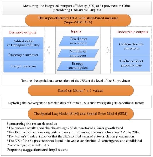
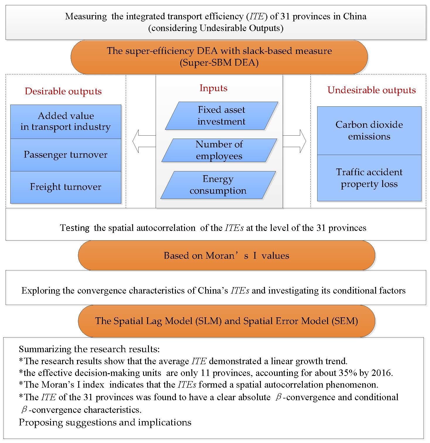
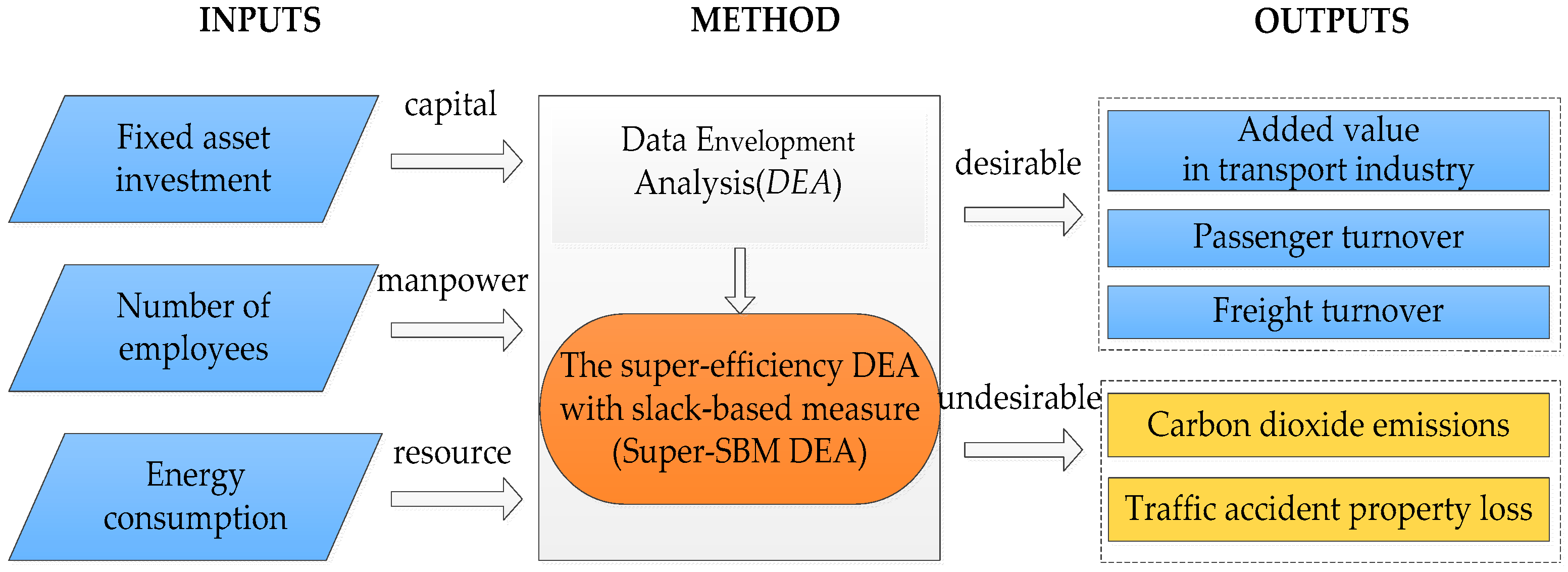
3. Models and Methods
3.1. Super-Efficiency Data Envelopment Analysis Model with Slack-Based Measure Considering Undesirable Outputs
3.2. Spatial Autocorrelation Model
3.3. Spatial Convergence Model
4. Empirical Analysis
4.1. Evaluation Index Selection and Data Sources
4.2. Results Analysis and Discussion
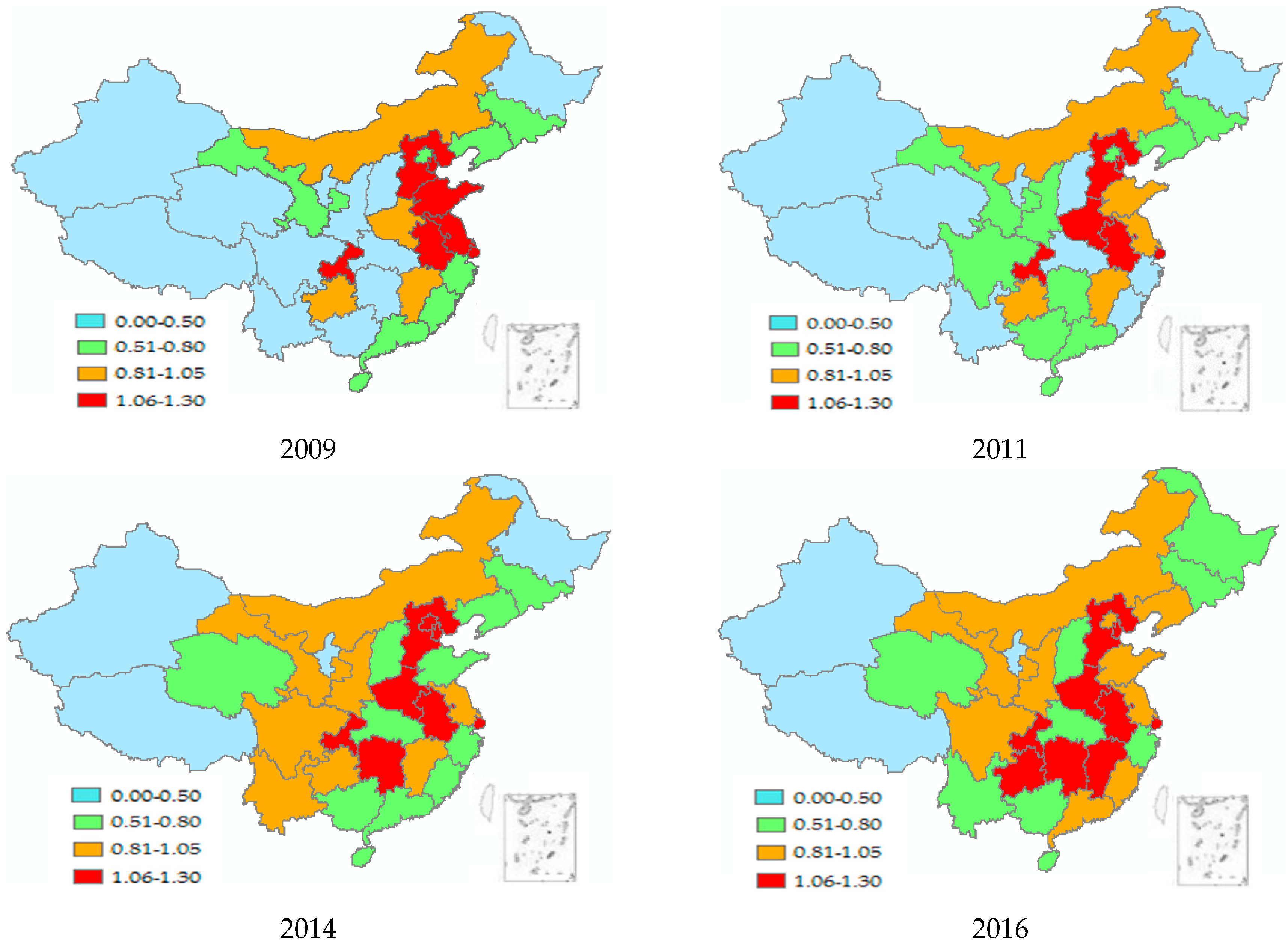
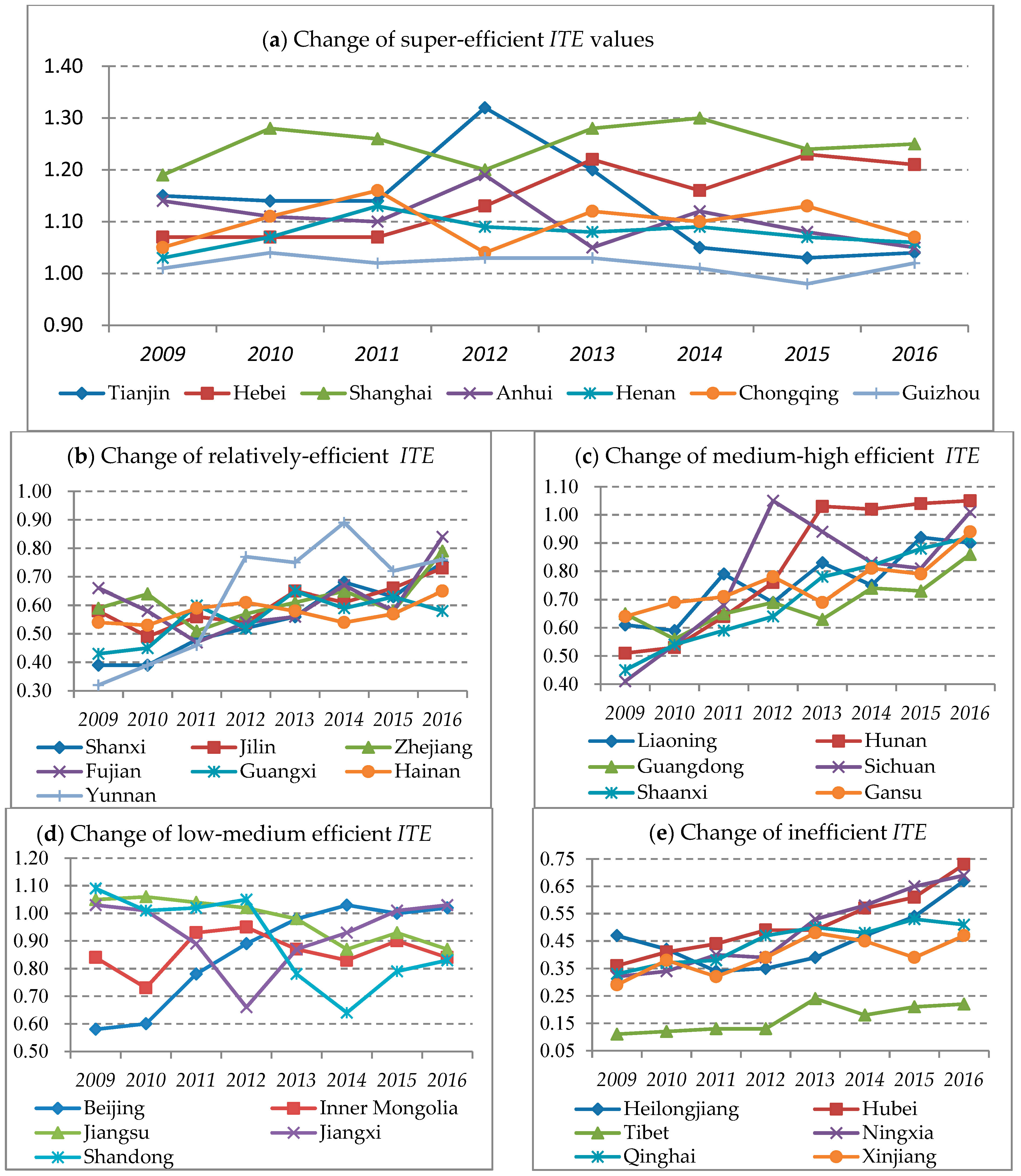
4.2.1. Evaluation of Integrated Transport Efficiency
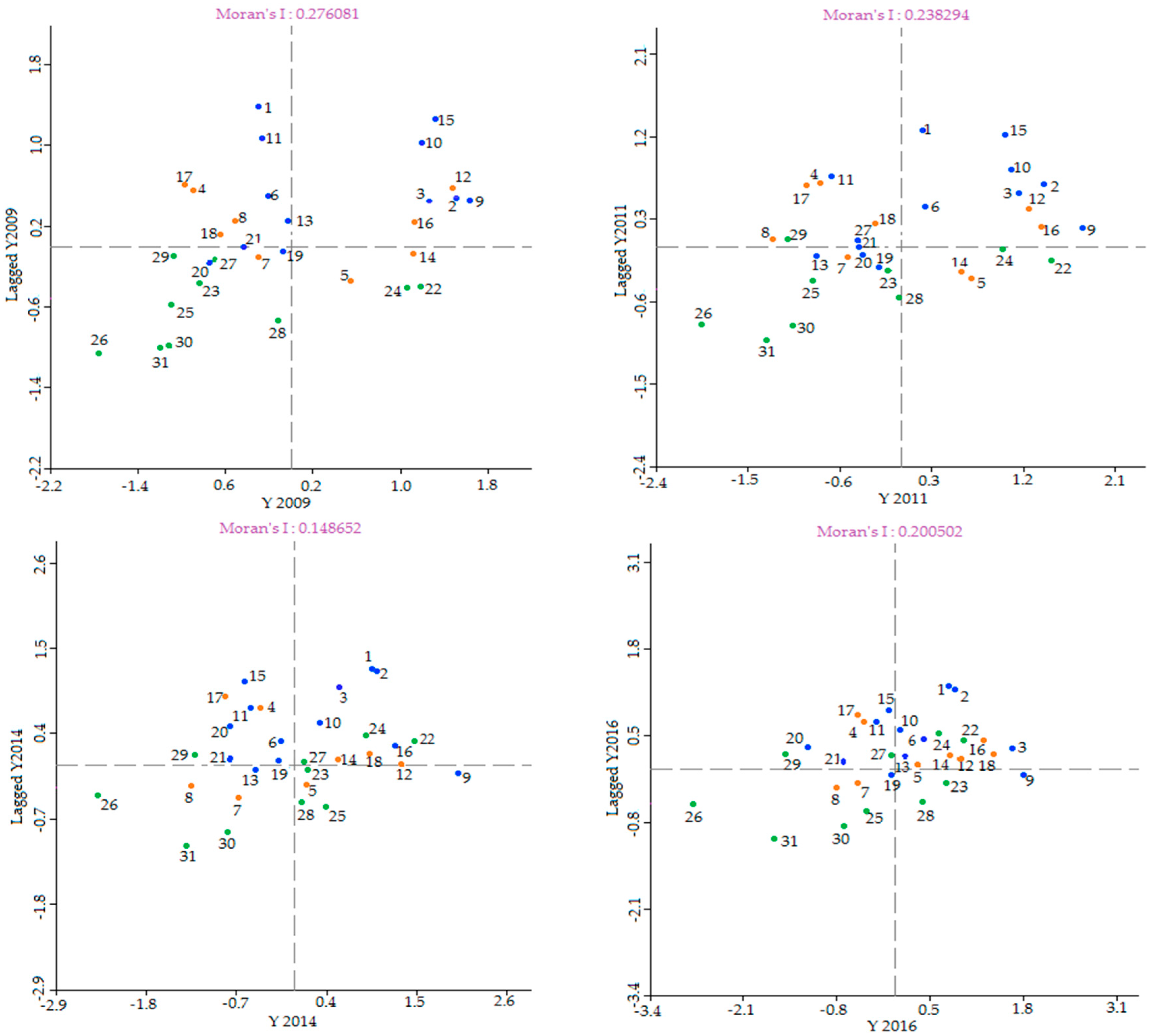
4.2.2. Spatial Autocorrelation Test and Aggregation Results
4.2.3. Convergence Analysis
5. Conclusions and Implications
Author Contributions
Funding
Acknowledgments
Conflicts of Interest
References
- Hadas, Y.; Ranjitkar, P. Modeling public-transit connectivity with spatial quality-of-transfer measurements. J. Transp. Geogr. 2012, 22, 137–147. [Google Scholar] [CrossRef]
- Wu, W.; Cao, Y.; Liang, S. Review of transport efficiency and its research trends from the transport geography perspectives. Prog. Geogr. 2013, 32, 243–250. [Google Scholar]
- Wu, J.; Ye, G.; Zhong, A. Efficiency Volatility and Influence Factors of Chinese Modern Transportation Industry Based on the Model of Cross-efficiency DEA and VAR. J. Transp. Syst. Eng. Inf. Technol. 2014, 14, 8–14. [Google Scholar]
- Woo, S.H.; Pettit, S.J.; Kwak, D.W.; Beresford, A.K.C. Seaport research: A structured literature review on methodological issues since the 1980s. Transp. Res. A Policy 2011, 45, 667–685. [Google Scholar] [CrossRef]
- Ruiz, T. Transport efficiency. Transp. Policy 2018. [Google Scholar] [CrossRef]
- Kotegawa, T.; Fry, D.; De Laurentis, D.; Puchaty, E. Impact of service network topology on air transportation efficiency. Transp. Res. Part C 2014, 40, 231–250. [Google Scholar] [CrossRef]
- Leng, Y.; Kou, C.; Zhou, N.; Li, Q.; Liang, Y.; Xu, Z.; Chen, S. Evaluation on Transfer Efficiency at Integrated Transport Terminals through Multilevel Grey Evaluation. Soc. Behav. Sci. 2012, 43, 587–594. [Google Scholar] [CrossRef]
- Palander, T. Environmental benefits from improving transportation efficiency in wood procurement systems. Transp. Res. Part D 2016, 44, 211–218. [Google Scholar] [CrossRef]
- Wang, H.; Liu, J.; Liu, K.; Zhang, J.; Wang, Z. Sensitivity analysis of traffic efficiency in restricted channel influenced by the variance of ship speed. Proc. Inst. Mech. Eng. Part M J. Eng. Marit. Environ. 2018, 232, 212–224. [Google Scholar] [CrossRef]
- Fei, M.; Xiao, D.L.; Sun, Q.; Liu, F.; Wang, W.; Bai, L. Regional Differences and Spatial Aggregation of Sustainable Transport Efficiency: A Case Study of China. Sustainability 2018, 10, 2399. [Google Scholar]
- Barnum, D.T.; Karlaft, M.G.; Tandon, S. Improving the efficiency of metropolitan area transit by joint analysis of its multiple providers. Transp. Res. Part E 2011, 47, 1160–1176. [Google Scholar] [CrossRef]
- Carlucci, F.; Cirà, A.; Coccorese, P. Measuring and Explaining Airport Efficiency and Sustainability: Evidence from Italy. Sustainability 2018, 10, 400. [Google Scholar] [CrossRef]
- Zhang, L.L.; Wu, W.; Liu, B.Q. Evaluation and analysis of highway transportation efficiency in the Yangtze River Delta based on DEA-Malmquist. J. Univ. Chin. Acad. Sci. 2017, 34, 712–718. [Google Scholar]
- Gao, P.; Sun, Z.J.; Lau, Y. Measuring Water Transport Efficiency in the Yangtze River Economic Zone, China. Sustainability 2017, 9, 2278. [Google Scholar] [Green Version]
- Joanna, G.; Wysoki’nska, Z. Transport accessibility in light of the DEA method. Comp. Econ. Res. 2014, 17, 55–70. [Google Scholar]
- Jain, P.; Cullinane, S.; Cullinane, K. The impact of governance development models on urban rail efficiency. Transp. Res. Part A 2008, 42, 1238–1250. [Google Scholar] [CrossRef]
- Peter, W.; Barros, C.P.; Figueiredo, O. Efficiency and productive slacks in urban transportation modes: A two-stage SDEA-Beta Regression approach. Util. Policy 2016, 41, 31–39. [Google Scholar]
- Tavassoli, M.; Faramarzi, G.R.; Saen, R.F. Efficiency and effectiveness in airline performance using a SBM-NDEA model in the presence of shared input. J. Air Transp. Manag. 2014, 34, 146–153. [Google Scholar] [CrossRef]
- Fu, J.; Jenelius, E. Transport efficiency of off-peak urban goods deliveries: A Stockholm pilot study. Case Stud. Transp. Policy 2018, 6, 156–166. [Google Scholar] [CrossRef]
- Dalmo, M.; Peter, W. Brazil’s rail freight transport: Efficiency analysis using two-stage DEA and cluster-driven public policies. Socio-Econ. Plan. Sci. 2017, 59, 26–42. [Google Scholar]
- Wua, J.; Zhu, Q.; Chu, J.; Liang, H.L. Measuring energy and environmental efficiency of transportation systems in China based on a parallel DEA approach. Transp. Res. Part D 2016, 48, 460–472. [Google Scholar] [CrossRef]
- Correia, E.; Carvalho, H.; Azevedo, S.G.; Govindan, K. Maturity models in supply chain sustainability: A systematic literature review. Sustainability 2017, 9, 64. [Google Scholar] [CrossRef]
- Centobelli, P.; Cerchione, R.; Esposito, E. Developing the WH2 framework for environmental sustainability in logistics service providers: A taxonomy of green initiatives. J. Clean. Prod. 2017, 165, 1063–1077. [Google Scholar] [CrossRef]
- Bi, G.; Wang, P.; Yang, F.; Liang, L. Energy and Environmental Efficiency of China’s Transportation Sector: A Multidirectional Analysis Approach. Math. Probl. Eng. 2014, 2014, 539596. [Google Scholar] [CrossRef]
- Liu, H.; Zhang, Y.; Zhu, Q.; Chu, J. Environmental efficiency of land transportation in China: A parallel slack-based measure for regional and temporal analysis. J. Clean. Prod. 2017, 142, 867–876. [Google Scholar] [CrossRef]
- Guanghui, Z.; William, C.; Yixiang, Z. Measuring energy efficiency performance of China’s transport sector: A data envelopment analysis approach. Expert Syst. Appl. 2014, 2, 709–722. [Google Scholar]
- Song, M.; Zheng, W.; Wang, Z. Environmental efficiency and energy consumption of highway Transportation systems in China. Int. J. Prod. Econ. 2016, 181, 441–449. [Google Scholar] [CrossRef]
- Li, G.; Huang, D.; Li, Y. China’s input-output efficiency of water-energy-food nexus based on the Data Envelopment Analysis (DEA) model. Sustainability 2016, 8, 927. [Google Scholar] [CrossRef]
- Bian, Y.; He, P.; Xu, H. Estimation of potential energy saving and carbon dioxide emission reduction in China based on an extended non-radial DEA approach. Energy Policy 2013, 63, 962–971. [Google Scholar] [CrossRef]
- Yang, Q.; Wan, X.; Ma, H. Assessing green development efficiency of municipalities and provinces in China integrating models of super-efficiency DEA and Malmquist index. Sustainability 2015, 7, 4492–4510. [Google Scholar] [CrossRef]
- Menegaki, A.N. Growth and renewable energy in Europe: Benchmarking with data envelopment analysis. Renew. Energy 2013, 60, 363–369. [Google Scholar] [CrossRef]
- Jia, S.; Wang, C.; Li, Y. The urbanization efficiency in Chendu City: An estimation based on a three-stage DEA model. Phys. Chem. Earth 2017, 101, 59–69. [Google Scholar] [CrossRef]
- Chang, Y.T.; Zhang, N.; Danao, D.; Zhang, N. Environmental efficiency analysis of transportation system in China: A non-radial DEA approach. Energy Policy 2013, 58, 277–283. [Google Scholar] [CrossRef]
- Centobelli, P.; Cerchione, R.; Esposito, E. Environmental Sustainability and Energy-Efficient Supply Chain Management: A Review of Research Trends and Proposed Guidelines. Energies 2018, 11, 275. [Google Scholar] [CrossRef]
- Zhou, P.; Ang, B.W. Linear programming models for measuring economy-wide energy efficiency performance. Energy Policy 2008, 38, 2911–2916. [Google Scholar] [CrossRef]
- Xin, D.; Cen, Y.; Lu, A. DEA Model-Based Efficiency Analysis for Road Transport of China’s 31 Provinces. J. Transp. Syst. Eng. Inf. Technol. 2011, 6, 25–29. [Google Scholar]
- Li, J.; Zuo, Y. Evaluation and analysis of highway transportation efficiency based on supper-efficiency DEA method. J. Transp. Inf. Saf. 2015, 1, 127–132. [Google Scholar]
- Wu, Q.; Song, J.; Ju, P.; Bao, X.; Du, K. Spatial Distribution of Provincial Integrated Transport Efficiency in China. Econ. Geogr. 2015, 35, 43–49. [Google Scholar]
- Meng, F.; Liu, G.; Yang, Z.; Casazza, M.; Cui, S.; Ulgiati, S. Energy efficiency of urban transportation system in Xiamen, China. An integrated approach. Appl. Energy 2017, 186, 234–248. [Google Scholar] [CrossRef]
- Fuglestvedt, J.; Berntesn, T.; Myhre, G.; Rypdal, K.; Skeie, R.B. Climate forcing from the transport sectors. Proc. Natl. Acad. Sci. USA 2007, 105, 454–458. [Google Scholar] [CrossRef] [PubMed]
- Wei, J.; Xia, W.; Guo, X.; Marinova, D. Urban transportation in Chinese cities: An efficiency assessment. Transp. Res. Part D 2013, 23, 20–24. [Google Scholar] [CrossRef]
- Tao, L.; Wenyue, Y.; Xiaoshu, C.; Zhang, H. Evaluating the impact of transport investment on the efficiency of regional integrated transport systems in China. Transp. Policy 2016, 45, 66–76. [Google Scholar]
- Yang, L.J.; Wei, W.; Su, Q.; Jiang, X.; Wei, Y. Evaluation of road transport efficiency in China during1997–2010 based on SBM-undesirable model. Prog. Geogr. 2013, 32, 1602–1611. [Google Scholar]
- Li, J.; Huang, X.; Yang, H.; Chuai, X.; Wu, C. Convergence of carbon intensity in the Yangtze River Delta, China. Habitat Int. 2017, 60, 58–68. [Google Scholar] [CrossRef]
- Xiao, Z.; Du, X.; Wu, C. Regional Difference and Evolution and Convergence of Innovation Capability in China: Research on Space and Factorial Levels. Sustainability 2017, 9, 1644. [Google Scholar] [CrossRef]
- Qin, C.; Ye, X.; Liu, Y. Spatial Club Convergence of Regional Economic Growth in Inland China. Sustainability 2017, 9, 1189. [Google Scholar] [CrossRef]
- Hao, Y.; Peng, H. On the convergence in China’s provincial per capita energy consumption: New evidence from a spatial econometric analysis. Energy Econ. 2017, 68, 31–43. [Google Scholar] [CrossRef]
- Charnes, A.; Cooper, W.W.; Rhodes, E. Measuring the efficiency of decision making units. Eur. J. Oper. Res. 1978, 2, 429–444. [Google Scholar] [CrossRef]
- Tone, K. A slacks-based measure of efficiency in data envelopment analysis. Eur. J. Oper. Res. 2001, 130, 498–509. [Google Scholar] [CrossRef] [Green Version]
- Song, M.; Zhang, L.; An, Q.; Wang, Z.; Li, Z. Statistical analysis and combination forecasting of environmental efficiency and its influential factors since China entered the WTO: 2002–2010–2012. J. Clean. Prod. 2013, 42, 42–51. [Google Scholar] [CrossRef]
- Anderson, P.; Petersen, N.C. A procedure for ranking efficient units in data envelopment analysis. Manag. Sci. 1993, 39, 1261–1264. [Google Scholar] [CrossRef]
- Parent, O.; LeSage, J.P. Spatial dynamic panel data models with random effects. Reg. Sci. Urban Econ. 2012, 42, 727–738. [Google Scholar] [CrossRef]
- Ma, F.; Wang, W.L.; Sun, Q.P.; Liu, F.; Li, X.D. Ecological Pressure of Carbon Footprint in Passenger Transport: Spatio-Temporal Changes and Regional Disparities. Sustainability 2018, 2, 317. [Google Scholar]
- Zhang, T.L.; Lin, G. On Moran’s I coefficient under heterogeneity. Comput. Stat. Data Anal. 2016, 95, 83–94. [Google Scholar] [CrossRef]
- National Bureau of Statistics of the People’s Republic of China. China Statistical Yearbook; China Statistics Press: Beijing, China, 2009–2016.
- National Statistics Bureau Energy Statistics Division. China Energy Statistics Yearbook; China Statistics Press: Beijing, China, 2009–2016.
- Li, J.; Jing, M.T.; Yuan, Q.M. Estimation of carbon emission and driving factors in Beijing-Tianjin-Hebei traffic under green development. J. Arid Land Resour. Environ. 2018, 7, 36–42. [Google Scholar]
- Cai, J. Analysis of Influence Factors of Road Transportation Demand Based on Bayesian Structural Equation Model. Chin. J. Manag. Sci. 2015, s1, 386–390. [Google Scholar]
- Yuan, C.W.; Zhang, S.; Jiao, P.; Wu, D. Temporal and spatial variation and influencing factors research on total factor efficiency for transportation carbon emissions in China. Resour. Sci. 2017, 39, 687–697. [Google Scholar]
- Fang, G.B.; Ma, H.M.; Song, G.J. Analysis of Energy Efficiency and Its Influence Factors in China’s Transportation—Based on the Three-phase DEA and GWR Methods. Stat. Inf. Forum 2016, 11, 59–67. [Google Scholar]


| Energy Type | Raw Coal | Coke | Crude | Fuel Oil |
|---|---|---|---|---|
| Standard Coal Conversion Factor (kgce/kg or m3) | 0.7143 | 0.9714 | 1.4286 | 1.4286 |
| CO2 emission factor (kg CO2/kg or m3) | 0.7559 | 0.8550 | 0.5857 | 0.6185 |
| Energy Type | Petrol | Kerosene | Diesel | Natural Gas |
| Standard Coal Conversion Factor (kgce/kg or m3) | 1.4714 | 1.4714 | 1.4571 | 1.4286 |
| CO2 emission factor (kg CO2/kg or m3) | 2.93 | 0.5714 | 0.5921 | 0.4483 |
| Index | Minimal | Maximal | Mean | Standard Deviation | |
|---|---|---|---|---|---|
| inputs | Fixed asset investment | 78.89 | 3516.28 | 918.68 | 643.47 |
| Number of employees | 3290 | 635,533 | 178,217.08 | 117,576.54 | |
| Energy consumption | 114.83 | 20,275.60 | 1656.10 | 3174.61 | |
| desirable outputs | added value in transport industry | 21.19 | 3209.72 | 892.34 | 676.16 |
| Passenger turnover | 29.98 | 2998.23 | 771.99 | 554.23 | |
| Freight turnover | 35.34 | 21,801.65 | 4772.51 | 4455.83 | |
| undesirable outputs | Carbon dioxide emissions | 78.08 | 13,787.41 | 1126.15 | 2158.73 |
| Traffic accident property loss | 290.54 | 10,726.59 | 3392.20 | 2255.92 |
| Province | 2009 | 2010 | 2011 | 2012 | 2013 | 2014 | 2015 | 2016 | Average ITE |
|---|---|---|---|---|---|---|---|---|---|
| Beijing | 0.58 | 0.60 | 0.78 | 0.89 | 0.98 | 1.03 | 1.00 | 1.02 | 0.86 |
| Tianjin | 1.15 | 1.14 | 1.14 | 1.32 | 1.20 | 1.05 | 1.03 | 1.04 | 1.13 |
| Hebei | 1.07 | 1.07 | 1.07 | 1.13 | 1.22 | 1.16 | 1.23 | 1.21 | 1.15 |
| Shanxi | 0.39 | 0.39 | 0.48 | 0.52 | 0.56 | 0.68 | 0.63 | 0.75 | 0.55 |
| Inner Mongolia | 0.84 | 0.73 | 0.93 | 0.95 | 0.87 | 0.83 | 0.90 | 0.84 | 0.86 |
| Liaoning | 0.61 | 0.59 | 0.79 | 0.69 | 0.83 | 0.75 | 0.92 | 0.90 | 0.76 |
| Jilin | 0.58 | 0.49 | 0.56 | 0.54 | 0.65 | 0.61 | 0.66 | 0.73 | 0.60 |
| Heilongjiang | 0.47 | 0.42 | 0.34 | 0.35 | 0.39 | 0.47 | 0.54 | 0.67 | 0.46 |
| Shanghai | 1.19 | 1.28 | 1.26 | 1.20 | 1.28 | 1.30 | 1.24 | 1.25 | 1.25 |
| Jiangsu | 1.05 | 1.06 | 1.04 | 1.02 | 0.98 | 0.87 | 0.93 | 0.87 | 0.98 |
| Zhejiang | 0.59 | 0.64 | 0.51 | 0.57 | 0.61 | 0.65 | 0.58 | 0.79 | 0.62 |
| Anhui | 1.14 | 1.11 | 1.10 | 1.19 | 1.05 | 1.12 | 1.08 | 1.05 | 1.11 |
| Fujian | 0.66 | 0.58 | 0.47 | 0.54 | 0.56 | 0.67 | 0.58 | 0.84 | 0.61 |
| Jiangxi | 1.03 | 1.01 | 0.89 | 0.66 | 0.87 | 0.93 | 1.01 | 1.03 | 0.93 |
| Shandong | 1.09 | 1.01 | 1.02 | 1.05 | 0.78 | 0.64 | 0.79 | 0.83 | 0.90 |
| Henan | 1.03 | 1.07 | 1.13 | 1.09 | 1.08 | 1.09 | 1.07 | 1.06 | 1.08 |
| Hubei | 0.36 | 0.41 | 0.44 | 0.49 | 0.49 | 0.57 | 0.61 | 0.73 | 0.51 |
| Hunan | 0.51 | 0.53 | 0.64 | 0.76 | 1.03 | 1.02 | 1.04 | 1.05 | 0.82 |
| Guangdong | 0.65 | 0.56 | 0.65 | 0.69 | 0.63 | 0.74 | 0.73 | 0.86 | 0.69 |
| Guangxi | 0.43 | 0.45 | 0.60 | 0.52 | 0.65 | 0.59 | 0.63 | 0.58 | 0.56 |
| Hainan | 0.54 | 0.53 | 0.59 | 0.61 | 0.58 | 0.54 | 0.57 | 0.65 | 0.58 |
| Chongqing | 1.05 | 1.11 | 1.16 | 1.04 | 1.12 | 1.10 | 1.13 | 1.07 | 1.10 |
| Sichuan | 0.41 | 0.54 | 0.68 | 1.05 | 0.94 | 0.83 | 0.81 | 1.01 | 0.76 |
| Guizhou | 1.01 | 1.04 | 1.02 | 1.03 | 1.03 | 1.01 | 0.98 | 1.02 | 1.02 |
| Yunnan | 0.32 | 0.39 | 0.46 | 0.77 | 0.75 | 0.89 | 0.72 | 0.76 | 0.63 |
| Tibet | 0.11 | 0.12 | 0.13 | 0.13 | 0.24 | 0.18 | 0.21 | 0.22 | 0.17 |
| Shaanxi | 0.45 | 0.54 | 0.59 | 0.64 | 0.78 | 0.82 | 0.88 | 0.92 | 0.70 |
| Gansu | 0.64 | 0.69 | 0.71 | 0.78 | 0.69 | 0.81 | 0.79 | 0.94 | 0.76 |
| Ningxia | 0.32 | 0.34 | 0.40 | 0.39 | 0.53 | 0.58 | 0.65 | 0.69 | 0.49 |
| Qinghai | 0.33 | 0.37 | 0.38 | 0.47 | 0.50 | 0.48 | 0.53 | 0.51 | 0.45 |
| Xinjiang | 0.29 | 0.38 | 0.32 | 0.39 | 0.48 | 0.45 | 0.39 | 0.47 | 0.40 |
| National Avg. ITE | 0.67 | 0.68 | 0.72 | 0.76 | 0.79 | 0.79 | 0.80 | 0.86 |
| Year | Moran’s I Value | Z Value | p Value |
|---|---|---|---|
| 2009 | 0.276 | 2.588 | 0.010 |
| 2010 | 0.265 | 2.667 | 0.011 |
| 2011 | 0.238 | 2.343 | 0.012 |
| 2012 | 0.240 | 2.384 | 0.010 |
| 2013 | 0.211 | 2.169 | 0.023 |
| 2014 | 0.149 | 1.986 | 0.030 |
| 2015 | 0.194 | 1.977 | 0.035 |
| 2016 | 0.201 | 2.181 | 0.023 |
| Year | 2009 | 2011 | 2014 | 2016 |
|---|---|---|---|---|
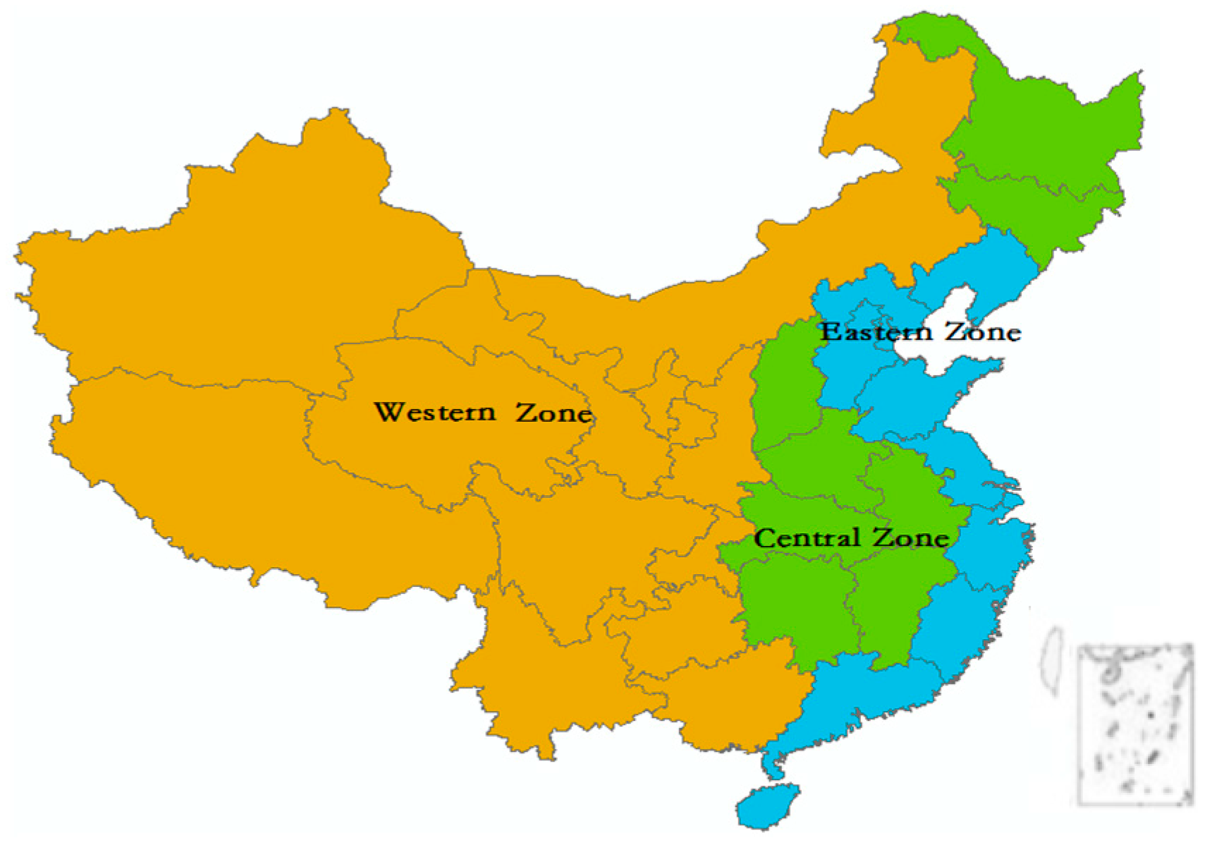
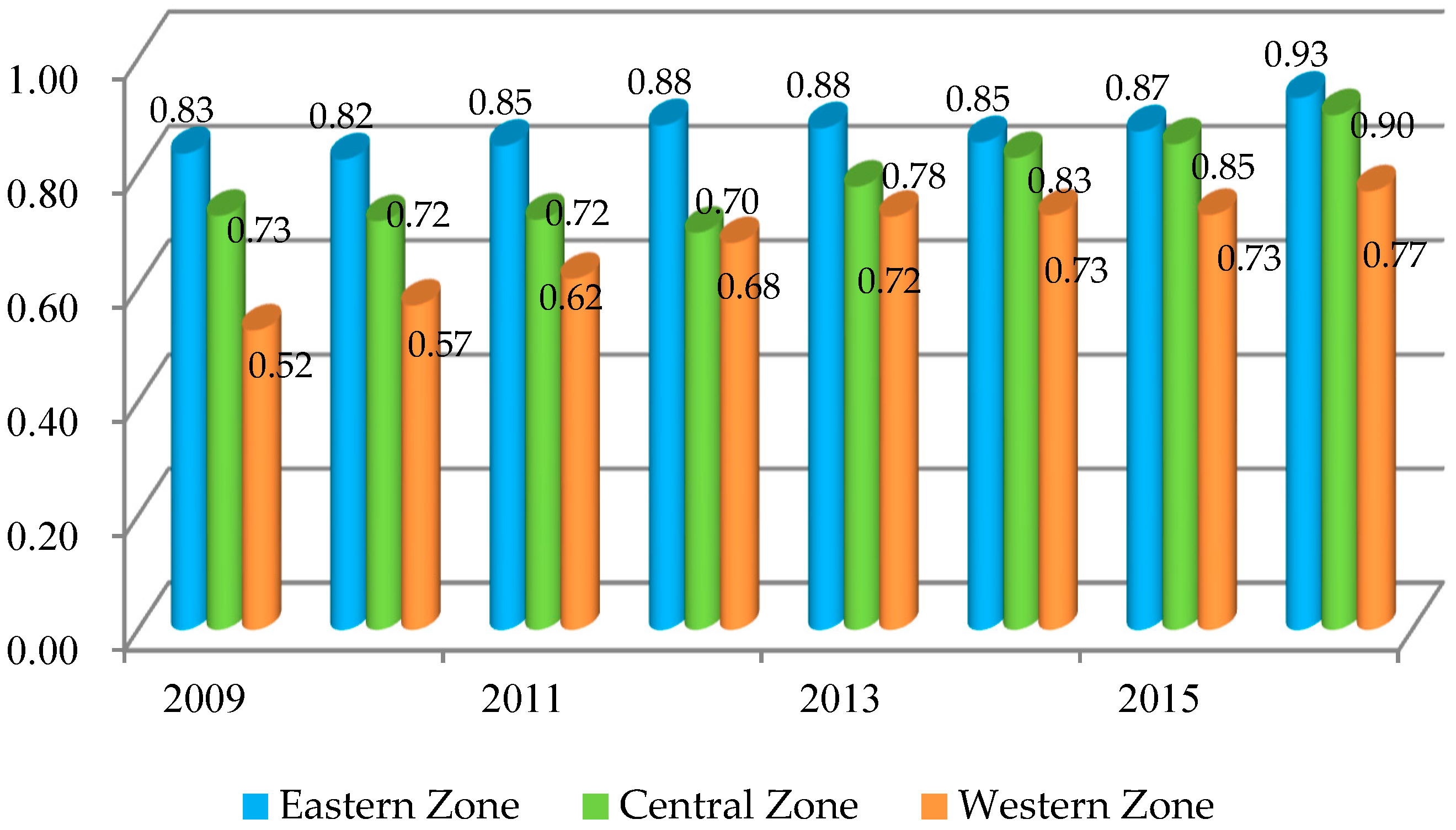
| H-H aggregation | Tianjin, Hebei, Shanghai, Jiangsu, Anhui, Shandong, Henan | Beijing, Tianjin, Hebei, Liaoning, Shanghai, Jiangsu, Anhui, Shandong, Henan | Beijing, Tianjin, Hebei, Jiangsu, Anhui, Jiangxi, Henan, Hunan, Chongqing, Guizhou, Shanxi | Beijing, Tianjin, Hebei, Jiangxi, Inner Mongolia, Liaoning, Anhui, Fujian, Jiangxi, Henan, Hunan, Chongqing, Guizhou |
| L-H aggregation | Beijing, Shanxi, Liaoning, Fujian, Heilongjiang, Zhejiang, Hubei, Hunan, Hainan | Shanxi, Hainan, Heilongjiang, Zhejiang, Hubei, Hunan, Shaanxi, Ningxia | Shanxi, Liaoning, Zhejiang, Hubei, Shandong, Hainan, Guangdong, Guangxi, Ningxia | Shanxi, Zhejiang, Hubei, Shandong, Guangxi, Hainan, Shaanxi, Ningxia |
| L-L aggregation | Jilin, Guangdong, Guangxi, Tibet, Yunnan, Sichuan, Shaanxi, Gansu, Ningxia, Qinghai, Xinjiang. | Jilin, Fujian, Guangdong, Guangxi, Tibet, Sichuan, Gansu, Yunnan, Qingha, Xinjiang, | Jilin, Henan, Heilongjiang, Fujian, Qinghai, Xinjiang. | Jilin, Yunnan, Tibet, Heilongjiang, Guangdong, Qinghai, Xinjiang. |
| H-L aggregation | Inner Mongolia, Jiangxi, Guizhou, Chongqing, | Inner Mongolia, Jiangxi, Guizhou, Chongqing, | Inner Mongolia, Shanghai, Gansu, Sichuan, Yunnan. | Shanghai, Gansu, Sichuan |
| LM_Error (p Value) | Robust LM_Error (p Value) | LM_Lag (p Value) | Robust LM_Lag (p Value) |
|---|---|---|---|
| 9.263 (0.023) | 7.381 (0.0014) | 5.279 (0.034) | 4.814 (0.0038) |
| β (t Value) | Spatial Residual Item (t Value) | Goodness of Fit | Maximum Likelihood | Convergence Speed% | Half Life Cycle |
|---|---|---|---|---|---|
| −0.1057 *** (−4.2603) | 0.274 *** (2.961) | 0.768 | 342.191 | 1.39 | 49.8 |
| Variable | Min | Max | Mean | Std. dev |
|---|---|---|---|---|
| led | 441.36 | 80,854.91 | 19,416.23 | 0.016 |
| gi | 0.005 | 0.124 | 0.021 | 0.027 |
| tids | 0.02 | 0.10 | 0.05 | 0.016 |
| ta | 0.03 | 1.52 | 0.82 | 0.52 |
| ti | 0.04 | 0.96 | 0.29 | 0.17 |
| ptse | 1993.80 | 3290.60 | 2298.06 | 920.72 |
| LM_Error (p Value) | Robust LM_Error (p Value) | LM_Lag (p Value) | Robust LM_Lag (p Value) |
|---|---|---|---|
| 8.419 (0.021) | 7.492 (0.018) | 6.994 (0.011) | 5.012 (0.005) |
| Variable | Double Fixed Effect (t Value) | Variable | Double Fixed Effect (t Value) |
|---|---|---|---|
| β | −0.385 *** (−10.429) | lngi | −0.118 *** (−3.075) |
| lnled | 0.102 ** (2.163) | lnsi | 0.0198 ** (0.207) |
| lntids | 0.149 *** (3.516) | lnptse | 0.024 ** (2.249) |
| lnti | 0.214 *** (3.843) | R–squared | 0.784 |
| Adj.R2 | 0.318 | Log-likelihood | 658.498 |
© 2018 by the authors. Licensee MDPI, Basel, Switzerland. This article is an open access article distributed under the terms and conditions of the Creative Commons Attribution (CC BY) license (http://creativecommons.org/licenses/by/4.0/).
Share and Cite
Ma, F.; Wang, W.; Sun, Q.; Liu, F.; Li, X. Integrated Transport Efficiency and Its Spatial Convergence in China’s Provinces: A Super-SBM DEA Model Considering Undesirable Outputs. Appl. Sci. 2018, 8, 1698. https://0-doi-org.brum.beds.ac.uk/10.3390/app8091698
Ma F, Wang W, Sun Q, Liu F, Li X. Integrated Transport Efficiency and Its Spatial Convergence in China’s Provinces: A Super-SBM DEA Model Considering Undesirable Outputs. Applied Sciences. 2018; 8(9):1698. https://0-doi-org.brum.beds.ac.uk/10.3390/app8091698
Chicago/Turabian StyleMa, Fei, Wenlin Wang, Qipeng Sun, Fei Liu, and Xiaodan Li. 2018. "Integrated Transport Efficiency and Its Spatial Convergence in China’s Provinces: A Super-SBM DEA Model Considering Undesirable Outputs" Applied Sciences 8, no. 9: 1698. https://0-doi-org.brum.beds.ac.uk/10.3390/app8091698