Quality Index of Supervised Data for Convolutional Neural Network-Based Localization

Department of System and Electronics Engineering, Toyota Central R&D Labs., Inc., 41-1, Yokomichi, Nagakute, Aichi 480-1192, Japan
*
Author to whom correspondence should be addressed.
Appl. Sci. 2019, 9(10), 1983; https://0-doi-org.brum.beds.ac.uk/10.3390/app9101983
Submission received: 4 February 2019
/
Revised: 26 April 2019
/
Accepted: 8 May 2019
/
Published: 15 May 2019
(This article belongs to the Special Issue Object Detection using Deep Learning for Autonomous Intelligent Robots)
Abstract
:Automated guided vehicles (AGVs) are important in modern factories. The main functions of an AGV are its own localization and object detection, for which both sensor and localization methods are crucial. For localization, we used a small imaging sensor named a single-photon avalanche diode (SPAD) light detection and ranging (LiDAR), which uses the time-of-flight principle and arrays of SPADs. The SPAD LiDAR works both indoors and outdoors and is suitable for AGV applications. We utilized a deep convolutional neural network (CNN) as a localization method. For accurate CNN-based localization, the quality of the supervised data is important. The localization results can be poor or good if the supervised training data are noisy or clean, respectively. To address this issue, we propose a quality index for supervised data based on correlations between consecutive frames visualizing the important pixels for CNN-based localization. First, the important pixels for CNN-based localization are determined, and the quality index of supervised data is defined based on differences in these pixels. We evaluated the quality index in indoor-environment localization using the SPAD LiDAR and compared the localization performance. Our results demonstrate that the index correlates well to the quality of supervised training data for CNN-based localization.
1. Introduction
Automated guided vehicles (AGVs) have important uses in modern factories. The main functions of an AGV are the localization and detection of pallets and cargo (see Figure 1). In large factories, sensors for AGVs must characterize targets over long ranges, as well as under different lighting conditions, because AGVs are often operated throughout the day both indoors and outdoors. To this end, light detection and ranging (LiDAR) in combination with cameras are useful in many scenarios. LiDAR [1,2] is a necessary technology to support the functionalities of AGVs and autonomous robots. A popular LiDAR sensor for autonomous robots is the one launched by Velodyne [1]. The Velodyne sensor HDL-64E outputs approximately one million points with 360 fields of view using multiple laser transmitters and receivers. However, these multiple transmitters and receivers hinder the incorporation and development of low-cost and small-sized sensors.
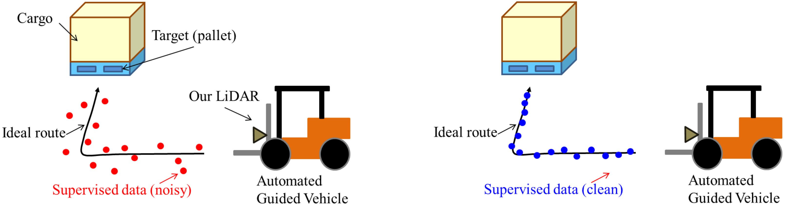
Recently, some approaches have leveraged deep convolutional neural networks (CNN) to perform localization [3,4,5,6]. However, to perform accurate CNN-based localization, the quality of supervised training data is important. If the supervised training data are noisy, poor localization results are obtained (see Figure 1 left), whereas clean supervised training data yields good localization results (see Figure 1 right).
To resolve these problems, we propose a quality index for supervised training data based on the correlations between consecutive frames that visualize the important pixels for CNN-based localization. First, we conducted a fundamental study to determine the important pixels for CNN-based localization. Our study showed that the important pixels differ depending on the quality of the supervised training data (see Figure 2). If the supervised training data are clean, the important pixels change gradually with the movement of an AGV. On the other hand, if the supervised training data are noisy, the important pixels change dramatically. We utilized these differences in pixel change rates to determine the quality of supervised data.
Secondly, we defined the quality index of supervised data based on the difference in important pixels. We evaluated our quality index in indoor environment localization using our small LiDAR sensor and compared the localization performance according to our index. Our results demonstrate that the index correlates to the quality of supervised training data for CNN-based localization.
Our results are presented as follows. Section 2 presents the related work, Section 3 presents our small LiDAR sensor, named single-photon avalanche diode (SPAD) LiDAR, and the quality index for supervised training data, and Section 4 presents the experimental findings and results through CNN-based localization. Finally, we conclude with suggestions for future research in Section 5.
2. Related Work
A number of works have focused on understanding CNN [7,8,9,10,11,12,13]. Yosinski [7] developed a tool to visualize the state of activations produced on each layer of a trained CNN. This tool can visualize the processes of activations as images or videos. Their work shows which activation reacts according to a particular input. They also developed a visualization tool for features at each layer of a CNN using regularized optimization. Their method enables recognition of the result of visualizations for an image classification task. Maaten and Hinton [8] proposed a dimensionality reduction technique, an improvement on stochastic neighbor embedding (SNE) named t-SNE, which is suitable for visualizing high-dimensional large datasets. The t-SNE enables us to see high-dimensional data on a low-dimensional space that we can plot. SNE converts the high-dimensional Euclidean distances between data into conditional probabilities. These probabilities represent the similarities among data. The t-SNE is a valuable tool for visualizing the result of a classification task. Some approaches attempt CNN visualization using a back-propagation-based approach. Springenberg [9] visualized CNN features based on a transpose convolution approach using un-pooling and transpose convolution. The VisualBackProp method by Bojarski [10] also uses deconvolution for visualization of a CNN. The method back-propagates the information of regions of relevance with a simultaneous increase in resolution by the deconvolution.
Recently, Zhou [11] showed that CNN can discover meaningful objects in the classification task. This work shows the features of CNN-captured objects at several levels of abstraction. For example, edges and textures are captured at near input layers, while objects and scenes are captured at near output layers. A randomized image patch was used to discover meaningful objects. Further, Zeiler and Fergus [12] explored the important pixels of each object in an image for a classification task. They used an input image that was occluded by a gray square and measured the difference in outputs. Zintgraf et al. [13] visualized the response of a deep neural network to a specific input using conditional and multivariate sampling. Their work shows differences in the response region in each major CNN architecture for a classification task. As discussed, most of the related works focus on visualization for classification tasks. On the other hand, our study focuses on the visualization of important pixels and the definition of a quality index for localization.
3. Approach
3.1. Small Imaging Sensor: SPAD LiDAR
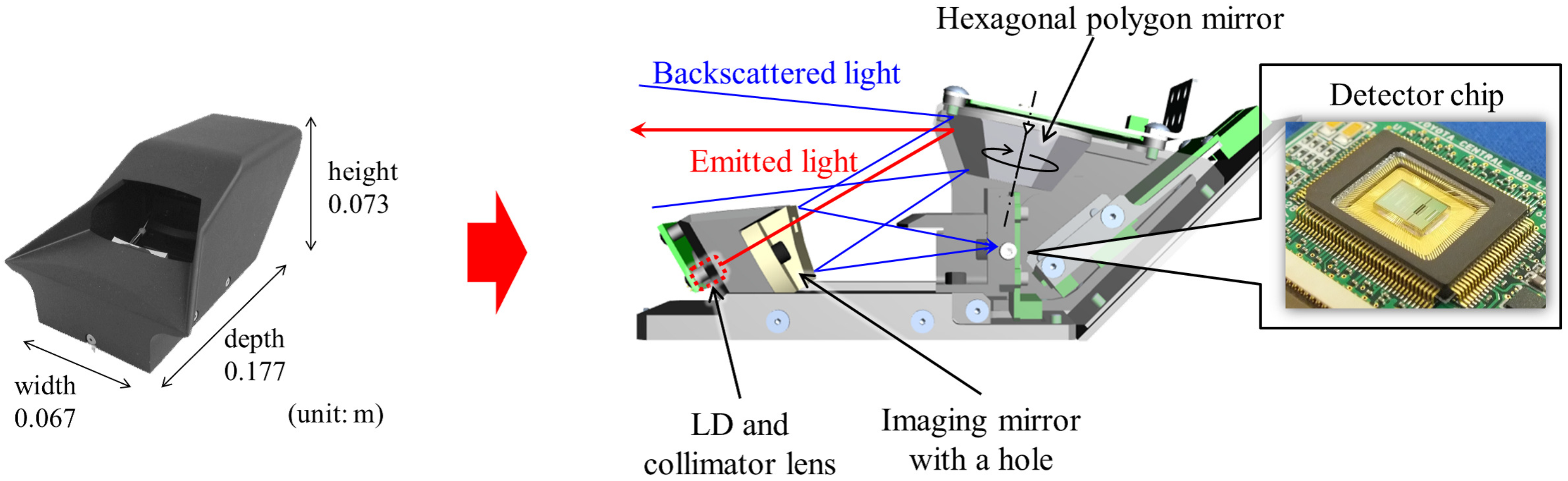
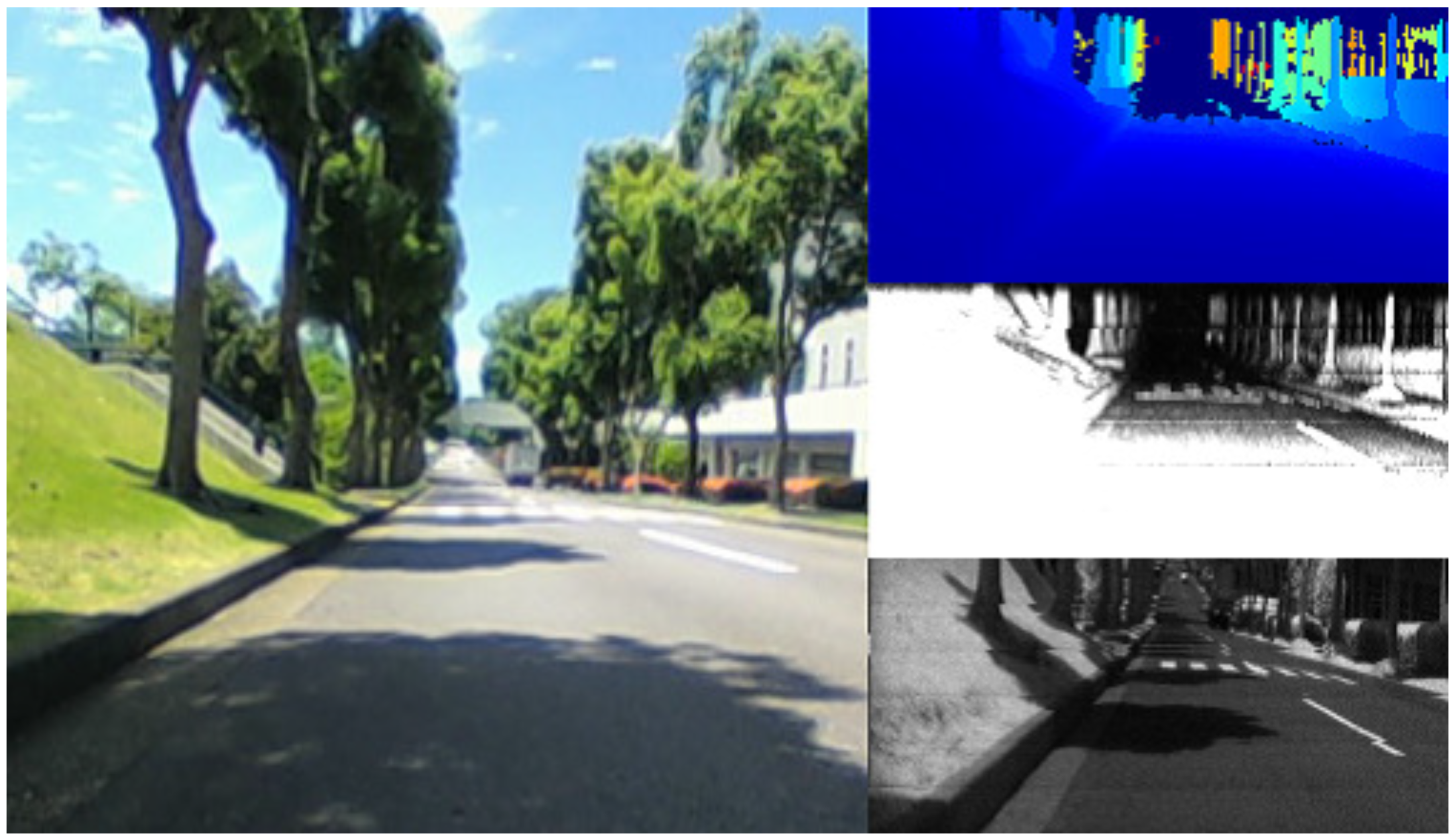
For localization of AGVs, we use a small imaging sensor named SPAD LiDAR [14]. Figure 3 and Table 1 show the configuration of the prototype. A laser diode (LD) with its collimator lens is installed behind an imaging mirror. The laser beam is emitted through a hole in the imaging lens and directed toward the targets after reflecting from a polygon mirror. Backscattered light returns through the same optical path and is focused on the photodetector, consisting of an array of 16 pixels. Since each facet of the hexagonal polygon mirror has a slightly different tilting angle, a horizontal scan, measuring 16 lines, can be achieved by rotating the polygon mirror and six vertical scans are achieved in one revolution. The 16 lines per vertical scan for the six vertical scans form a total of 96 lines of depth imaging, while 202 points are measured in the horizontal scan. The photodetector is a SPAD fabricated using the complementary metal oxide semiconductor (CMOS) process. The time-of-flight (TOF) is estimated based on time-correlated single photon counting (TCSPC), wherein the histogram of photon incident timing is generated and the peak is extracted to distinguish the back-scattered light from ambient light. The peak value is regarded as the reliability, while the peak position is the TOF in the histogram. Ambient light, regarded as the intensity, is measured with another 1D array of pixels and placed next to the pixels for TOF measurement where the laser beam has not fallen. As a result, three kinds of information—TOF, reliability, and intensity—are acquired with each pixel. An example of the acquired data as well as a reference image captured with a camera is shown in Figure 4.
3.2. Quality Index Based on Important Pixels for CNN-Based Localization
In this section, we describe the main components of our quality index approach, which are the visualization of important pixels (step 1) and comparison of important pixels (step 2). Figure 5 depicts the major components of our approach.
3.2.1. Step 1: Visualization of Important Pixels
Step 1 visualizes the important pixels for CNN-based localization. To clarify the important pixels for CNN-based localization, we used an occlusion-based approach, which replaces some original input pixels with other pixels, namely occlusion pixels. If the occluded pixels are important for localization, the localization result changes compared to the result that was obtained using the original input data. The occlusion-based approach compares the localization results obtained from the original input data and occluded input data. The occluded input is generated using a randomized patch. Figure 6 depicts examples of occluded data. Given the input data x, we augment the square patch, p, of size on x in a sliding window fashion. Each pixel of this square patch is a random value. If the pixels occluded by this patch are important for localization, the localization results become worse. We generated 16,512 augmented data per frame of the original raw data.
To reveal the important pixels for CNN-based localization, we compared the localization result obtained using the original raw data with the localization results obtained using the augmented data. If the pixels occluded by a randomized patch are important for localization, the difference between the localization results of raw data and augmented data becomes large. On the other hand, if the pixels occluded by a randomized patch are not important for localization, the difference between the localization results of raw data and augmented data becomes small.
We consider these differences as the importance of the pixel and define them as
where is the difference in the localization of raw data and augmented data, m is the number of layer, c is the number of outputs, l is the number of channels, and is the position of the randomized patch in the original image x. Figure 7 shows an example of the importance map produced by Equation (1). In the example given in Figure 7, the important pixels for localization are around a pallet.
3.2.2. Step 2: Quality Index
We define the quality index of supervised data using the co-efficiency of consecutive frames of the visualization result, which shows important pixels for localization. This is based on the assumption that if the supervised training data are of good quality, then the important pixels for CNN-based localization would change gradually in a factory situation. The quality index is defined by Equation (2).
where
These equations are used to calculate the correlation of consecutive visualized images. Here, w and h are the width and height of the image and I and T represent an image at the times t and , respectively. The other variables are indexes.
3.2.3. CNN-Based Localization
This section introduces the localization method based on the SPAD LiDAR and CNN. The localization method uses raw sensor data that can be acquired from the SPAD LiDAR and augmented data shown in Figure 6. The outputs of the localization are the position of a target. For example, in an application of AGVs, the targets are pallets in a warehouse.
Before localization, the method requires a CNN model in an environment. A CNN model is determined from supervised training data (e.g., motion capture data, drive data made by a human operator, or existing localization data). After producing a CNN model, the localization method uses only range data, peak intensity data, and monocular data for localization.
To explore the basic study of important pixels, we used a simple plain network architecture for our CNN that consists of three convolution layers, three pooling layers, and two fully connected layers. Our previous paper [15] presented the parameters of the network. The input data consist of three channels. The size of each data is 202 × 96 pixels. Before the first convolutional layer, the CNN resizes the input data to 112 × 112. The CNN has two output layers. One output layer is a classification output for the existence of a target. For example, in an AGV application, the target is a pallet, which the AGV must approach. The other output layer is a regression output for a 3D position and orientation of LiDAR.
For this multi-output structure, the CNN uses the multi-task loss function presented by Girshick [16] and Ren [17]. The loss function for the CNN is defined as
where denotes the classification loss for a true class u, and p is an estimated class. If there is a target in input data, then the true class becomes one. In addition, is the regression loss for a predicted position of the LiDAR, v is the ground truth position and orientation, and controls the balance between the classification loss and regression loss. In this paper, is empirically decided. The method minimizes the multi-task loss function.
4. Experiments
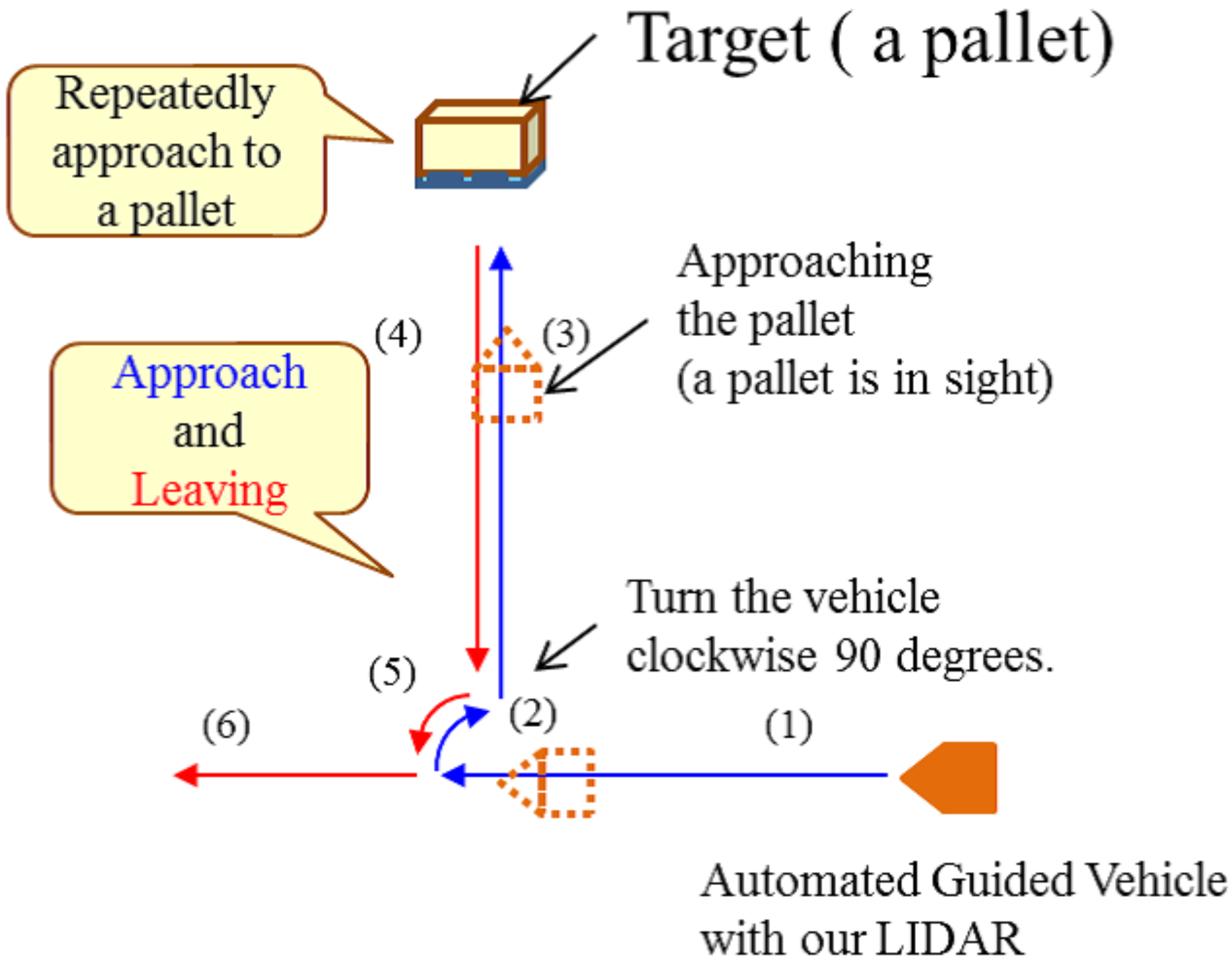
We evaluated our quality index for CNN-based localization in a set of indoor environment experiments. Figure 8 and Figure 9 show the assumed scenario of the experiments. Figure 8 depicts the typical trajectories of AGV. We named these trajectories as scenario 1. In a certain factory, an AGV equipped with the SPAD LiDAR approached a pallet. The AGV selected and lifted the cargo and then carried the cargo to another location repeatedly. Figure 9 is another scenario of AGV. Initially, the AGV equipped with the SPAD LiDAR moves in a straight line (see (1) in Figure 9). At this time, the pallet was out of sight of the SPAD LiDAR. Then, the AGV rotated by 90 degrees in a clockwise direction (see (2) in Figure 9) and approached the pallet. The pallet came within sight during the rotation. The AGV finally approached the pallet. We named these trajectories as scenario 2. We designed the experimental evaluation to show the following.
- Reveal important pixels for CNN-based localization.
- The index reflects the quality of supervised data for CNN-based localization.
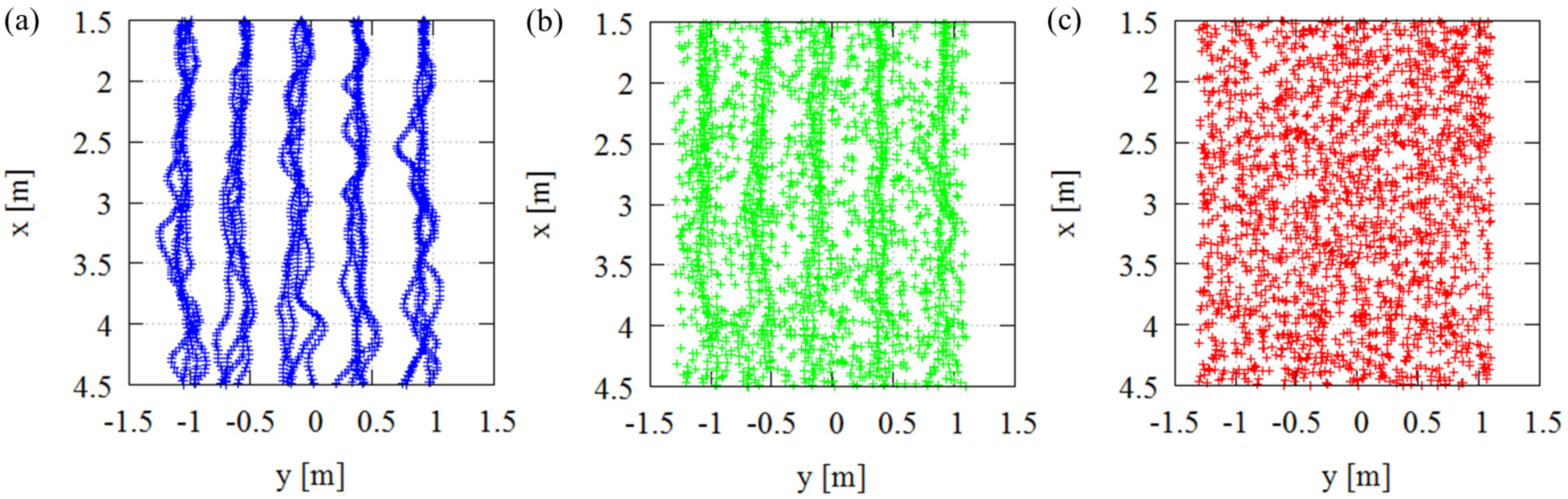
For this purpose, we collected and generated 11 types of supervised training datasets for each assumed scenario and named them datasets A–K. The first supervised data were the trajectories of an AGV captured by a motion capture system, as depicted in Figure 10a. We named this data as dataset A and used them to explore the important pixels in an ideal situation. Another ten supervised data were generated from the first data and were used to add noise to the original dataset A. We named these datasets B–K (see Table 2. These ten datasets differed in their noise ratios compared to the original data. Figure 10b shows examples of dataset F, which had mixed data of trajectories by motion capture and noise. We used this data to compare the important pixels of an ideal situation with that of a noisy situation. Dataset K consisted of only random noise, as depicted in Figure 10c. We used these datasets to compare differences in the important pixels. All data had multiple datasets for cross-validation with a leave-one-dataset-out technique.
All experiments were conducted using a robot operating system (ROS) [18] and TensorFlow [19]. ROS is an open-source meta-operating system that facilitates collaboration with many software packages, while TensorFlow is an open-source machine-learning framework. We created a driver of SPAD LiDAR for ROS and collected all the data. In addition, we implemented our CNN using TensorFlow. The CNN model named SPAD DCNN was presented in our previous paper [15]. This CNN model outputs localization results using the data of SPAD LiDAR as inputs.
4.1. Results
4.1.1. Important Pixels
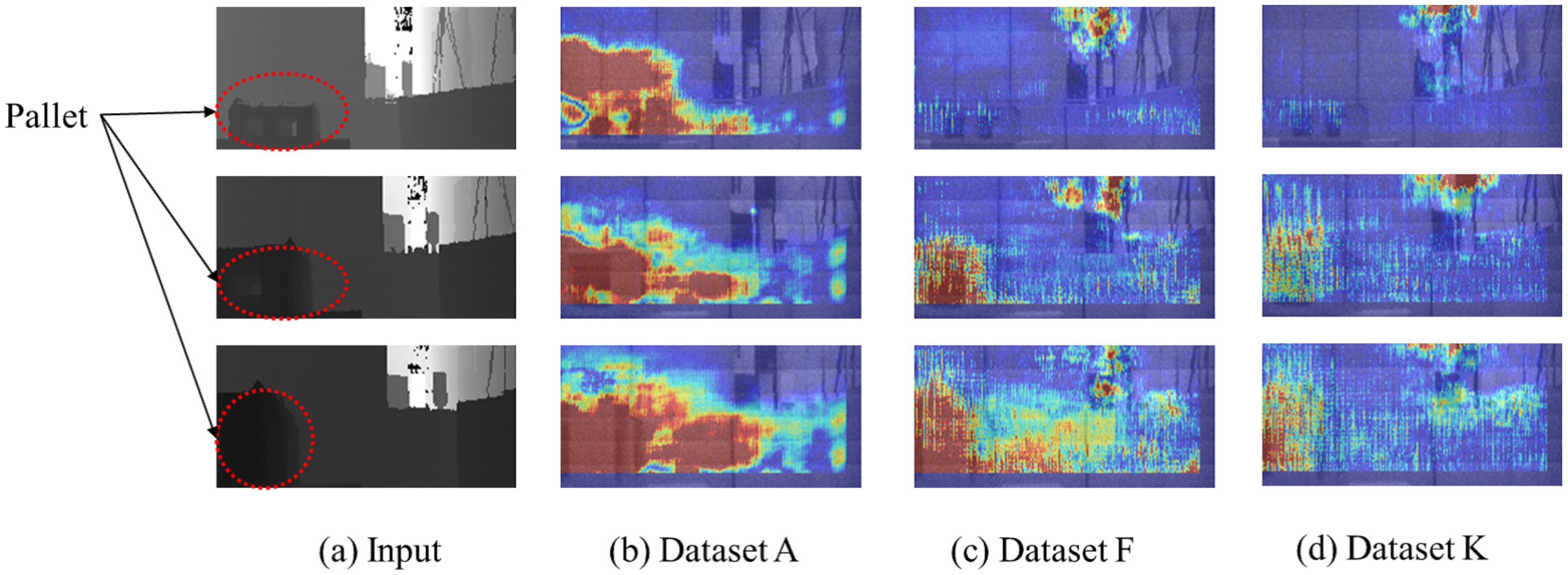
We visualize important pixels using trained CNN models [15], and the visualization method is described in Section 3.2.1. Figure 11 shows the results of important regions under different datasets in the assumed scenario 1. In the Figure 11, the red pixels are important for CNN-based localization. The blue pixels are unimportant for CNN-based localization. As the figures show, the important pixels of the CNN trained by random noise were scattered throughout the input images (see Figure 11c,d), while the important pixels of the CNN trained by motion capture data were gathered around the pallet that the AGV is approaching (see Figure 11b). This phenomenon implies that the important pixels of CNN-based localization varied according to the quality of the supervised localization data.
4.1.2. Quality Index and Localization
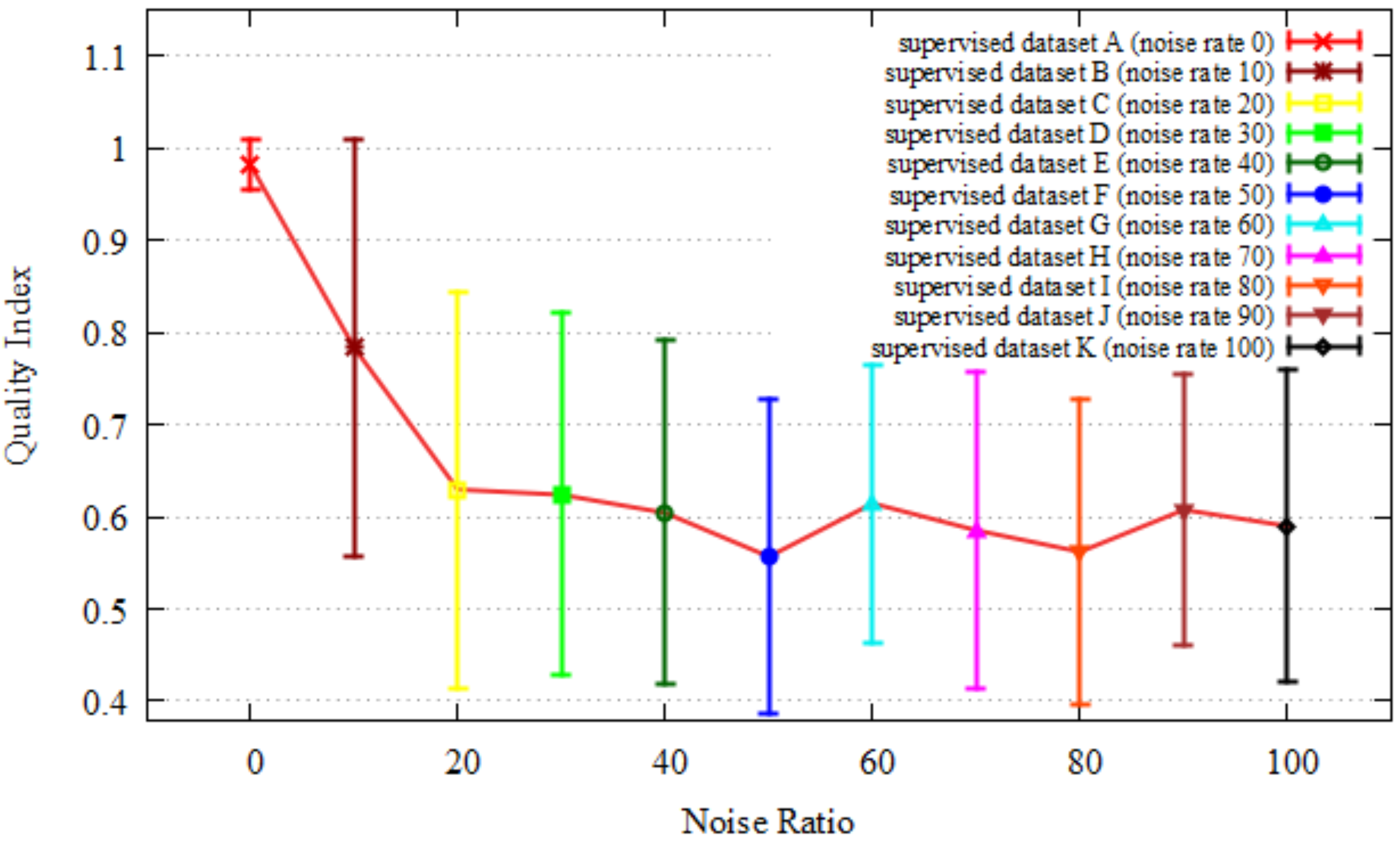
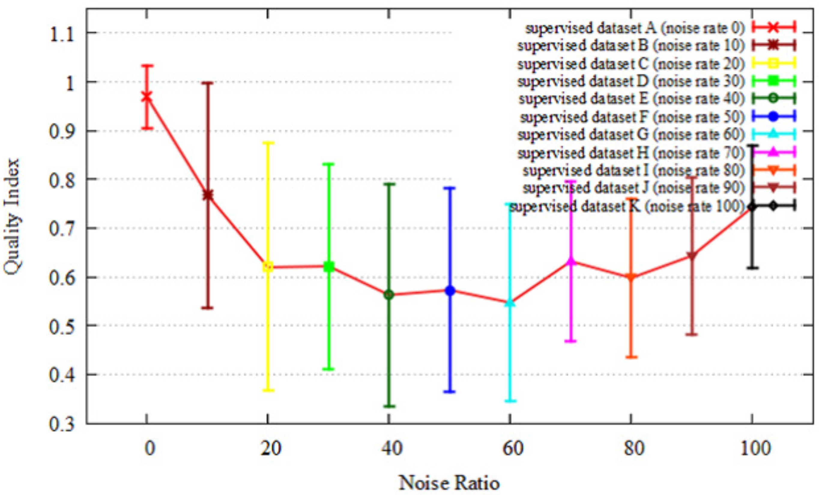
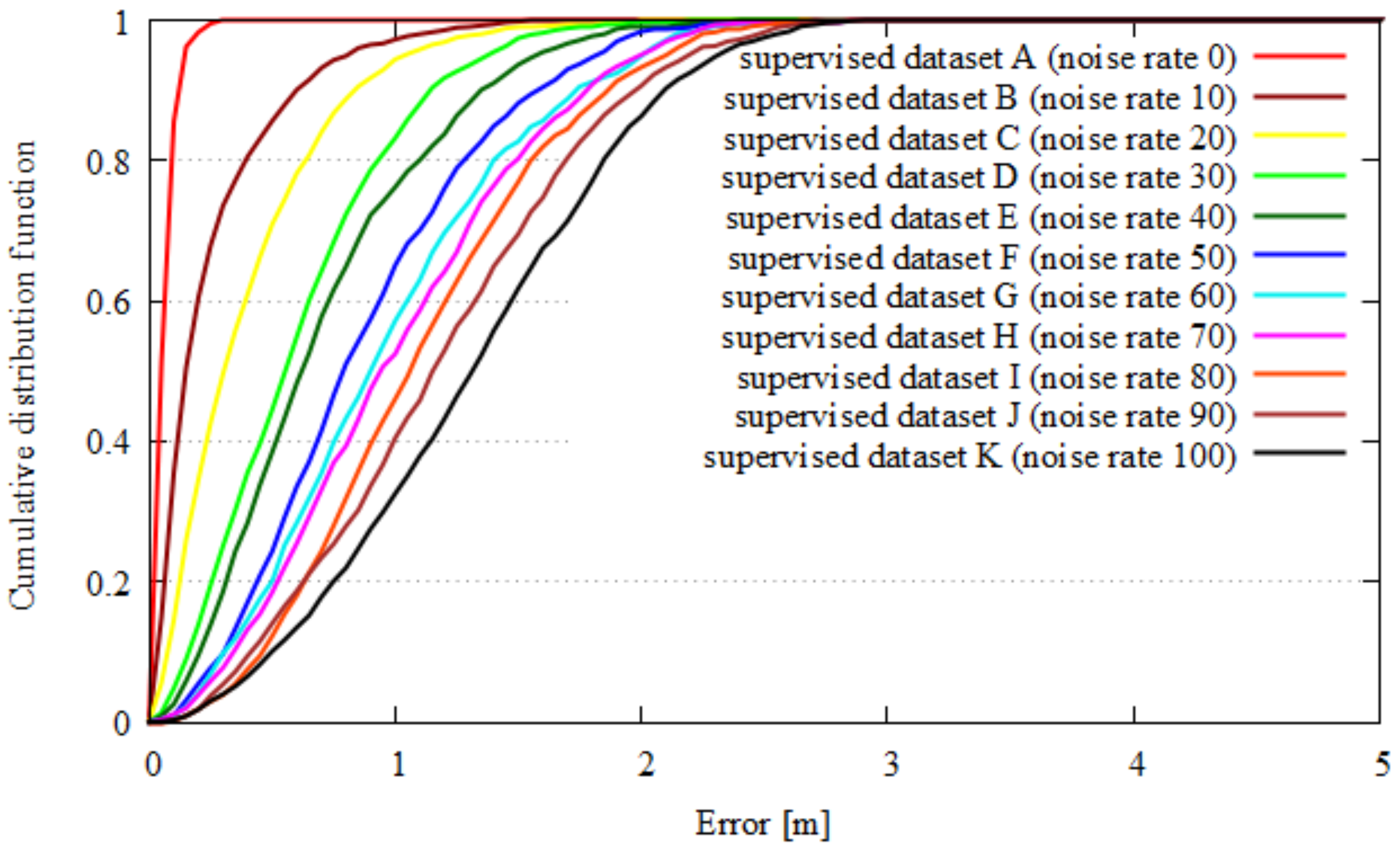
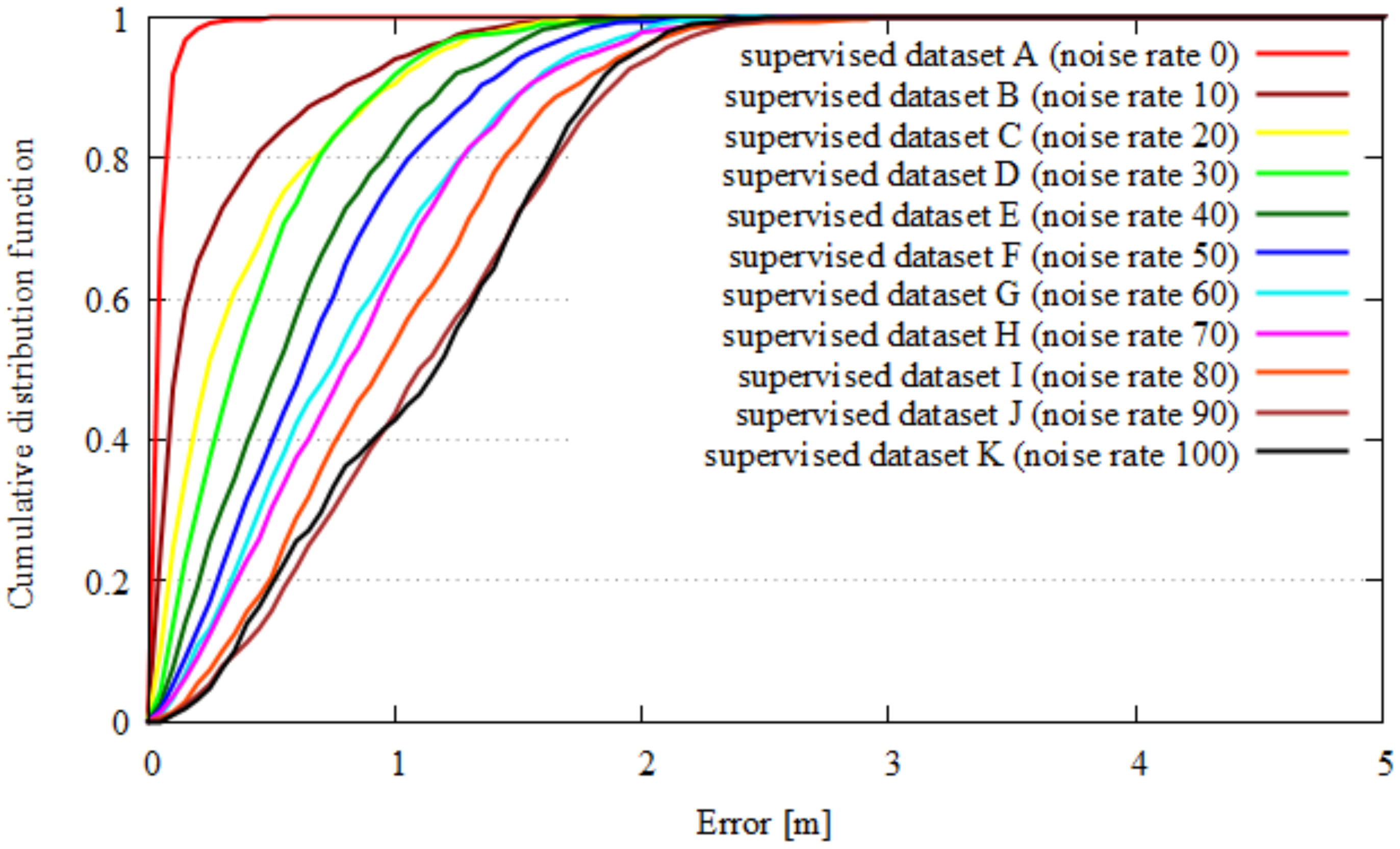
We evaluated our quality index for all the data from dataset A–K in the assumed scenarios 1 and 2. Figure 12 shows the results of the quality index evaluation of each dataset in scenario 1. Figure 13 shows the results of quality index evaluation of each dataset in scenario 2. Here, the x-axes depict the ratio of random noise on supervised data, and the Y-axes show the quality index. With an increase in the noise of supervised data, the quality index is decreased. From these results, our quality index identified noise up to 20 percent in scenario 1 and up to 10 percent in scenario 2. Figure 14 and Figure 15 show the localization results of each dataset. Here, the x-axis is the localization error, and the y-axis is the cumulative distribution function of the localization results. The localization results worsen with a decrease in quality index in both scenarios up to 20 percent noise.
5. Conclusions
As described in this paper, we identified the important pixels for CNN-based localization and presented a quality index for supervised data. The main contributions of this paper are the determination of important pixels for CNN-based localization and showing the differences in important pixels based on the quality of supervised data. The results show that our quality index correlates to noise rates up to 20 percent in experimental scenarios. The approach is most useful during the selection of supervised data, especially when some data includes noise. Possible extensions of this work include the improvement of supervised training data with noise using our quality index.
Author Contributions
M.S., H.M. and M.O. conceived and designed the prototype hardware of SPAD LiDAR; S.I., S.H. conceived and designed the driver software of SPAD LiDAR, DCNN-based localization, and Quality Index; S.I., S.H. and H.M. performed the experiments; S.I., M.S., S.H., H.M. and M.O. contributed to the development of the systems for the experiments.
Funding
This research received no external funding.
Conflicts of Interest
The authors declare no conflict of interest.
References
- Velodyne 3D LiDAR. Available online: https://velodynelidar.com/products.html (accessed on 28 January 2019).
- SICK 3D LiDAR. Available online: https://www.sick.com/us/en/detection-and-ranging-solutions/3d-lidar-sensors/c/g282752 (accessed on 28 January 2019).
- Kendall, A.; Grimes, M.; Cipolla, R. PoseNet: A Convolutional Network for Real-Time 6-DOF Camera Relocalization. In Proceedings of the International Conference on Computer Vision (ICCV), Santiago, Chile, 13–16 December 2015. [Google Scholar]
- Arroyo, R.; Alcantarilla, P.F.; Bergasa, L.M.; Romera, E. Fusion and Binarization of CNN Features for Robust Topological Localization across Seasons. In Proceedings of the IEEE/RSJ International Conference on Intelligent Robots and Systems (IROS), Daejeon, Korea, 9–14 October 2016. [Google Scholar]
- Naseer, T.; Burgard, W. Deep Regression for Monocular Camera-based 6-DoF Global Localization in Outdoor Environments. In Proceedings of the IEEE/RSJ International Conference on Intelligent Robots and Systems (IROS), Vancouver, BC, Canada, 24–28 September 2017. [Google Scholar]
- Porzi, L.; Penate-Sanchez, A.; Ricci, E.; Moreno-Noguer, F. Depth-aware Convolutional Neural Networks for accurate 3D Pose Estimation in RGB-D Images. In Proceedings of the IEEE/RSJ International Conference on Intelligent Robots and Systems (IROS), Vancouver, BC, Canada, 24–28 September 2017. [Google Scholar]
- Yosinski, J.; Clune, J.; Nguyen, A.; Fuchs, T.; Lipson, H. Understanding Neural Networks through Deep Visualization. In Proceedings of the International Conference on Machine Learning Workshops (ICML), Lille, France, 6–11 July 2015. [Google Scholar]
- Van der Maaten, L.; Hinton, G. Visualizing data using t-SNE. J. Mach. Learn. Res. 2018, 9, 2579–2605. [Google Scholar]
- Springenberg, J.T.; Dosovitskiy, A.; Brox, T.; Riedmiller, M. Striving for Simplicity: The All Convolutional Net. In Proceedings of the International Conference on Learning Representations Workshops (ICLR Workshops), San Diego, CA, USA, 7–9 May 2015. [Google Scholar]
- Bojarski, M.; Choromanska, A.; Choromanski, K.; Firner, B.; Jackel, L.; Muller, U.; Zieba, K. VisualBackProp: Visualizing CNNs for autonomous driving. arXiv 2016, arXiv:1611.05418. [Google Scholar]
- Zhou, B.; Khosha, A.; Lapedriza, A.; Oliva, A.; Torralba, A. Object Detectors Emerge in Deep Scene CNNs. In Proceedings of the International Conference on Learning Representations (ICLR), San Diego, CA, USA, 7–9 May 2015. [Google Scholar]
- Zeiler, M.D.; Fergus, R. Visualizing and Understanding Convolutional Networks. In Proceedings of the European Conference on Computer Vision (ECCV), Zurich, Switzerland, 6–12 September 2014. [Google Scholar]
- Zintgraf, L.M.; Cohen, T.S.; Adel, T.A.; Welling, M. Visualizing Deep Neural Network Decisions: Prediction Difference Analysis. In Proceedings of the International Conference on Learning Representations Workshops (ICLR Workshops), Toulon, France, 24–26 April 2017. [Google Scholar]
- Niclass, C.; Soga, M.; Matsubara, H.; Kato, S.; Kagami, M. A 100-m-range 10-frame/s 340x96-pixel time-of-flight depth sensor in 0.18 μm CMOS. IEEE J. Solid-State Circuits 2013, 48, 559–572. [Google Scholar] [CrossRef]
- Ito, S.; Hiratsuka, S.; Ohta, M.; Matsubara, H.; Ogawa, M. SPAD DCNN: Localization with Small Imaging LIDAR and DCNN. In Proceedings of the IEEE/RSJ International Conference on Intelligent Robots and Systems (IROS), Vancouver, BC, Canada, 24–28 September 2017. [Google Scholar]
- Girshick, R. Fast-R-CNN. arXiv 2015, arXiv:1504.08083. [Google Scholar]
- Ren, S.; He, K.; Girshick, R.; Sun, J. Faster R-CNN: Toward Real-Time Object Detection with Region Proposal Networks. arXiv 2015, arXiv:1506.01497. [Google Scholar] [CrossRef] [PubMed]
- Quigley, M.; Conley, K.; Gerkey, B.; Conley, K.; Faust, J.; Foote, T.; Leibs, J.; Berger, E.; Wheeler, R.; Ng, A. ROS: An open-source Robot Operating System. In Proceedings of the IEEE International Conference on Robotics and AutomationWorkshops (ICRAWorkshops), Kobe, Japan, 12–17 May 2009. [Google Scholar]
- Abadi, M.; Barham, P.; Chen, J.; Chen, Z.; Davis, A.; Dean, J.; Devin, M.; Ghemawat, S.; Irving, G.; Isard, M.; et al. TensorFlow: A system for large-scale machine learning. In Proceedings of the USENIX Symposium on Operating Systems Design and Implementation (OSDI), Savannah, GA, USA, 2–4 November 2016. [Google Scholar]
Figure 1.
Example of an assumed scenario for automated guided vehicles (AGVs) and problem statement.
Figure 1.
Example of an assumed scenario for automated guided vehicles (AGVs) and problem statement.

Figure 2.
Difference in important pixels.

Figure 3.
Single-photon avalanche diode (SPAD) light detection and ranging (LiDAR).

Figure 4.
Example of outputs of the prototype LiDAR sensor with a reference image in an outdoor environment: (top right) range data; (middle right) peak intensity data; (bottom right) monocular data. Left figure shows reference image obtained by a camera.
Figure 4.
Example of outputs of the prototype LiDAR sensor with a reference image in an outdoor environment: (top right) range data; (middle right) peak intensity data; (bottom right) monocular data. Left figure shows reference image obtained by a camera.

Figure 5.
Overview of the system.

Figure 6.
Example of augmented data. Randomized square patch, p is augmented to the original input image x.
Figure 6.
Example of augmented data. Randomized square patch, p is augmented to the original input image x.

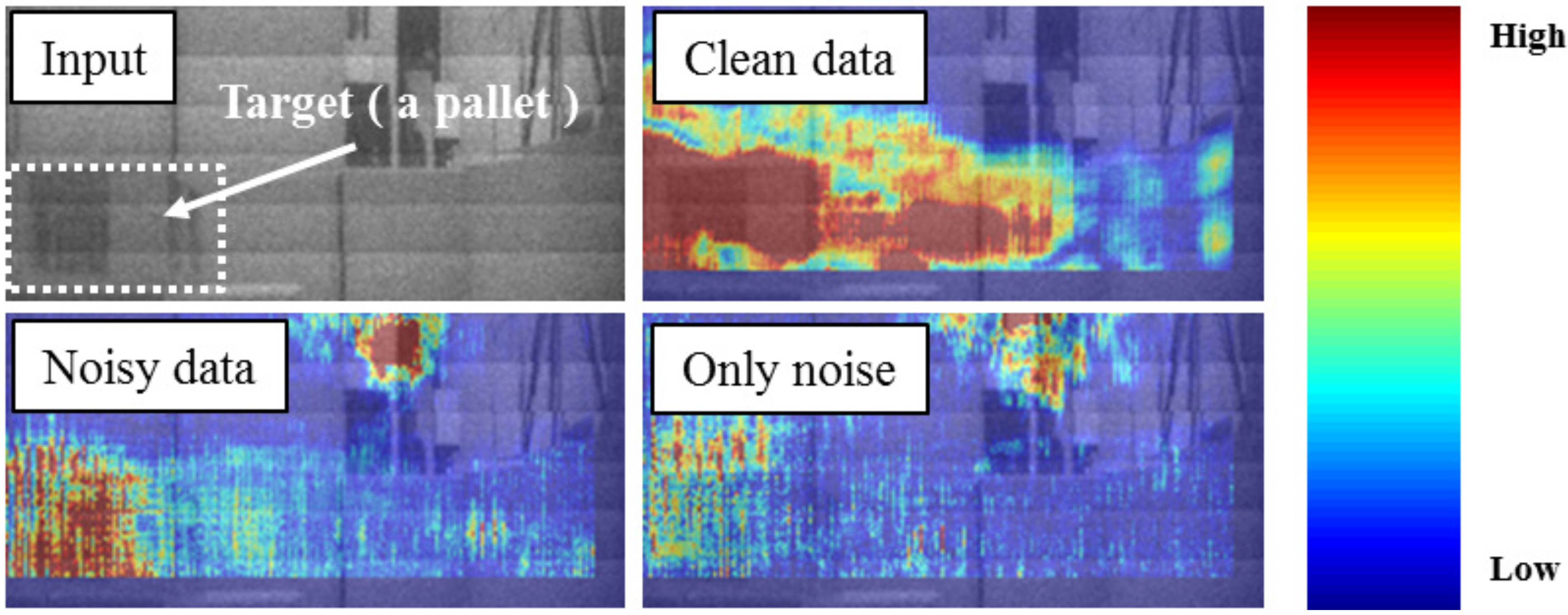
Figure 7.
Examples of raw input (top) and importance image (bottom). In this example, pixels around a pallet that the AGV approaches are important for convolutional neural network (CNN)-based localization.
Figure 7.
Examples of raw input (top) and importance image (bottom). In this example, pixels around a pallet that the AGV approaches are important for convolutional neural network (CNN)-based localization.

Figure 8.
Example of assumed scenario 1 for AGV. An AGV equipped with SPAD LiDAR automatically approaches a pallet and transports the pallet to another location.
Figure 8.
Example of assumed scenario 1 for AGV. An AGV equipped with SPAD LiDAR automatically approaches a pallet and transports the pallet to another location.

Figure 9.
Example of assumed scenario 2 for AGV. The AGV equipped with the SPAD LiDAR moves in a straight line. Then, the AGV rotates clockwise by 90 degrees. Finally, the AGV automatically approaches a pallet and transports the pallet to another location.
Figure 9.
Example of assumed scenario 2 for AGV. The AGV equipped with the SPAD LiDAR moves in a straight line. Then, the AGV rotates clockwise by 90 degrees. Finally, the AGV automatically approaches a pallet and transports the pallet to another location.

Figure 10.
Three examples of supervised training data collected for assumed scenario 1: (a) dataset A: AGV trajectories captured by motion capture, (b) dataset F: AGV trajectories with random noise, and (c) dataset K: only random noise data.
Figure 10.
Three examples of supervised training data collected for assumed scenario 1: (a) dataset A: AGV trajectories captured by motion capture, (b) dataset F: AGV trajectories with random noise, and (c) dataset K: only random noise data.

Figure 11.
Results of important pixels of CNN-based localization in the scenario 1: (a) input data of SPAD LiDAR, (b) important pixels using the CNN trained by dataset A, (c) important pixels using the CNN trained by dataset F, and (d) important pixels using the CNN trained by dataset K.
Figure 11.
Results of important pixels of CNN-based localization in the scenario 1: (a) input data of SPAD LiDAR, (b) important pixels using the CNN trained by dataset A, (c) important pixels using the CNN trained by dataset F, and (d) important pixels using the CNN trained by dataset K.

Figure 12.
Quality index of each dataset in scenario 1.

Figure 13.
Quality index of each dataset in scenario 2.

Figure 14.
Test error of each dataset in scenario 1.

Figure 15.
Test error of each dataset in scenario 2.


Table 1.
Main specifications of the single-photon avalanche diode (SPAD) light detection and ranging (LiDAR).
Table 1.
Main specifications of the single-photon avalanche diode (SPAD) light detection and ranging (LiDAR).
| Specifications | |
|---|---|
| Pixel Resolution | 202 × 96 pixels |
| FOV | 55 × 9 degrees |
| Frame rate | 10 frames/s |
| Size | W 0.067 × H 0.073 × D 0.177 m |
| Range | 70 m |
| Wavelength | 905 nm |
| Frequency | 133 kHz |
| Peak power | 45 W |
| TOF measurement | Pulse type |
| Laser | Class 1 laser |
| Distance resolution | 0.035 m (short-range mode), 0.070 m (long-range mode) |
Table 2.
Overview of all datasets.
| All Dataset | |
|---|---|
| Dataset A | Original motion capture dataset |
| Dataset B | 10% of data were replaced with noise |
| Dataset C | 20% of data were replaced with noise |
| Dataset D | 30% of data were replaced with noise |
| Dataset E | 40% of data were replaced with noise |
| Dataset F | 50% of data were replaced with noise |
| Dataset G | 60% of data were replaced with noise |
| Dataset H | 70% of data were replaced with noise |
| Dataset I | 80% of data were replaced with noise |
| Dataset J | 90% of data were replaced with noise |
| Dataset K | All of data were replaced with noise |
© 2019 by the authors. Licensee MDPI, Basel, Switzerland. This article is an open access article distributed under the terms and conditions of the Creative Commons Attribution (CC BY) license (http://creativecommons.org/licenses/by/4.0/).
Share and Cite
MDPI and ACS Style
Ito, S.; Soga, M.; Hiratsuka, S.; Matsubara, H.; Ogawa, M. Quality Index of Supervised Data for Convolutional Neural Network-Based Localization. Appl. Sci. 2019, 9, 1983. https://0-doi-org.brum.beds.ac.uk/10.3390/app9101983
AMA Style
Ito S, Soga M, Hiratsuka S, Matsubara H, Ogawa M. Quality Index of Supervised Data for Convolutional Neural Network-Based Localization. Applied Sciences. 2019; 9(10):1983. https://0-doi-org.brum.beds.ac.uk/10.3390/app9101983
Chicago/Turabian StyleIto, Seigo, Mineki Soga, Shigeyoshi Hiratsuka, Hiroyuki Matsubara, and Masaru Ogawa. 2019. "Quality Index of Supervised Data for Convolutional Neural Network-Based Localization" Applied Sciences 9, no. 10: 1983. https://0-doi-org.brum.beds.ac.uk/10.3390/app9101983
Note that from the first issue of 2016, this journal uses article numbers instead of page numbers. See further details here.