An EKF-Based Method and Experimental Study for Small Leakage Detection and Location in Natural Gas Pipelines


1
School of Energy and Building Engineering, Harbin University of Commerce, Harbin 150028, China
2
Department of Engineering Technology, College of Technology, University of Houston, Houston, TX 77204, USA
*
Author to whom correspondence should be addressed.
Appl. Sci. 2019, 9(15), 3193; https://0-doi-org.brum.beds.ac.uk/10.3390/app9153193
Submission received: 12 July 2019
/
Revised: 1 August 2019
/
Accepted: 1 August 2019
/
Published: 5 August 2019
(This article belongs to the Special Issue Recent Advances in Structural Health Monitoring and Nondestructive Testing in Civil Engineering)
Abstract
:Small leaks in natural gas pipelines are hard to detect, and there are few studies on this problem in the literature. In this paper, a method based on the extended Kalman filter (EKF) is proposed to detect and locate small leaks in natural gas pipelines. First, the method of a characteristic line is used to establish a discrete model of transient pipeline flow. At the same time, according to the basic idea of EKF, a leakage rate is distributed to each segment of the discrete model to obtain a model with virtual multi-point leakage. As such, the virtual leakage rate becomes a component of the state variables in the model. Secondly, system noise and measurement noise are considered, and the optimal hydraulic factors such as leakage rate are estimated using EKF. Finally, by using the idea of an equivalent pipeline, the actual leakage rate is calculated and the location of leakage on the pipeline is assessed. Simulation and experimental results show that this method can consistently predict the leakage rate and location and is sensitive to small leakages in a natural gas pipeline.
1. Introduction
Natural gas is a kind of high-quality, efficient, clean energy and raw material. Since the 1970s, the development of natural gas in the world has been accelerated, and the research on gas exploitation, transportation, and storage has received increasing attention [1,2,3,4,5,6,7]. Nowadays, natural gas pipelines account for almost half of the total length of pipelines in the world. Natural gas is poisonous and explosive. Therefore, it is important that natural gas pipelines are maintained in a safe manner. Leakages are the major causes of in-service natural gas pipeline accidents. In practice, natural gas pipeline leakages can be divided into two types—sudden and rapid leakages with a high leakage rate, and slow leakages with a low leakage rate, also known as seepage.
Sudden leakages are mostly caused by third-party earth work, heavy vehicle rolling, geological changes, and impacts [8,9]. There is extensive literature on sudden leakage detection [10,11,12,13], such as the commonly used negative pressure wave (NPW) method [14,15,16] and the fiber-optic-based method [17,18]. The principle of NPW is that when leaks develop in a natural gas pipeline, the gas density near the leak point will decrease rapidly. This phenomenon results in a negative pressure wave which propagates through the gas from the leak point. The NPW method often employs pressure sensors or other types of sensors that can detect wave propagation. Thanks to the recent development in structural health monitoring [19,20,21,22,23,24,25,26] and damage detection [27,28,29,30,31,32,33], many new types of sensors, such as piezoceramic transducers [34,35,36,37,38,39] and fiber optic sensors [40,41,42,43], have been developed for civil infrastructure. Because of their high bandwidth and low cost, piezoceramic transducers have been applied to pipeline monitoring [44,45,46]. On the other hand, because of their distributive nature and small size, fiber optic sensors are often reported for pipeline monitoring [47,48,49]. In the NPW method, these sensors are installed upstream and downstream of a pipeline to detect negative pressure waves [50,51,52,53,54]. The signal captured by these pressure sensors can be processed to determine whether there is a gas leak. Fiber-optic-based methods usually use distributed fiber optical sensors to detect leakages in natural gas pipelines; a distributed fiber optical sensor installed along the pipeline can detect the temperature variation or vibrations caused by leakage. The commonality of these two methods is the utilization of sensors. This leads to a potential problem that if the sensors are not accurate enough, it is highly possible to miss the alarms for small leakages.
Slow small leakages (seepage) usually occur in weak links of the pipelines, such as welding seams, flanges, or valves [55,56,57], and they are difficult to detect due to their concealment. In addition, pipelines are subject to corrosion [58,59,60], erosion [61], and cracking [62,63,64], which may also cause small leakages at the initial stage. Currently, there are only limited studies in this area [65,66]. At present, the effective method for small leakages is based on the real-time model method. Compared with other leakage detection methods, the real-time model method can provide all the characteristics of pipeline flow and fluid properties. It also considers the impact of physical properties of pipelines. In addition, the real-time model considers the influence of system noise and measurement noise and has advantages in small leakage detection. However, it also has some disadvantages, such as complex computation and slow convergence.
The Kalman filter is a kind of filtering algorithm that estimates the required states through algorithms from the observation quantity related to the extracted signal, however, it can only be used for linear systems. The Kalman filter that can estimate states for a nonlinear system is called the extended Kalman filter (EKF) [67]. Continuous nonlinear equations need to be linearized first when using EKF. The EKF has the advantages of fast convergence and high accuracy in state estimation [68,69,70,71]. This paper proposes an EKF-based method for small leakage detection and location in natural gas pipelines.
Most researchers working in this topic approach the leakage detection problem from the research field of control. The main limitation in the extant literature is about the applicability of different control and detection methods. Complementary to the previous efforts, the authors of this paper approach this topic as subject matter experts in pipe leakage detection. We understand that both the NPW method and the fiber-optic-based method are widely used and able to obtain reasonably good leakage detection results. These two methods do not need to establish a pipeline model. They mainly process signals and identify patterns for real-time leakage detection. However, these two methods mainly work well with the common sudden and rapid leakage detection. They perform poorly with the slow and small leakage. EKF-based method is essentially a real-time modeling method. This method requires pipeline models. The computation is complex and converges slowly. Therefore, this method is not suitable for sudden and rapid leakage detection. On the other hand, a real-time model can provide a pipeline’s flow characteristics and fluid properties and consider pipeline physical properties as well. In addition, a real-time model considers the effect of system noise and measurement noise. Its working principle determines its advantage in slow and small leakage detection. The Kalman filter has the advantages of fast convergence and high precision in terms of state estimation. This compensates for the original shortcomings in the real-time model method such as slow convergence. Therefore, it is adopted for real-time leakage detection in this paper.
The rest of the paper is organized as follows. Section 2 proposes the pipeline transient flow model containing the virtual multi-point leakages. Section 3 elaborates the mathematics for the state estimation by EKF. Section 4 explains the calculation of the actual leakage rate and location. Section 5 verifies the model with a simulation example. In Section 6, a physical experiment is conducted to validate the effectiveness of the proposed method. Section 7 concludes the paper.
2. The Pipeline Transient Flow Model Containing the Virtual Multi-Point Leakages
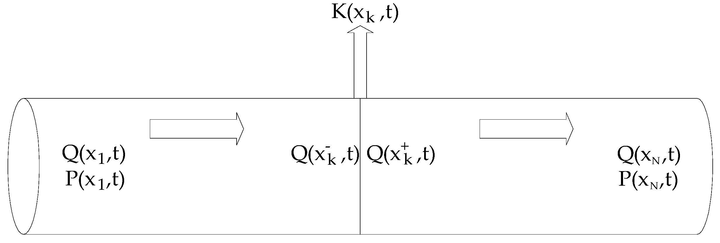
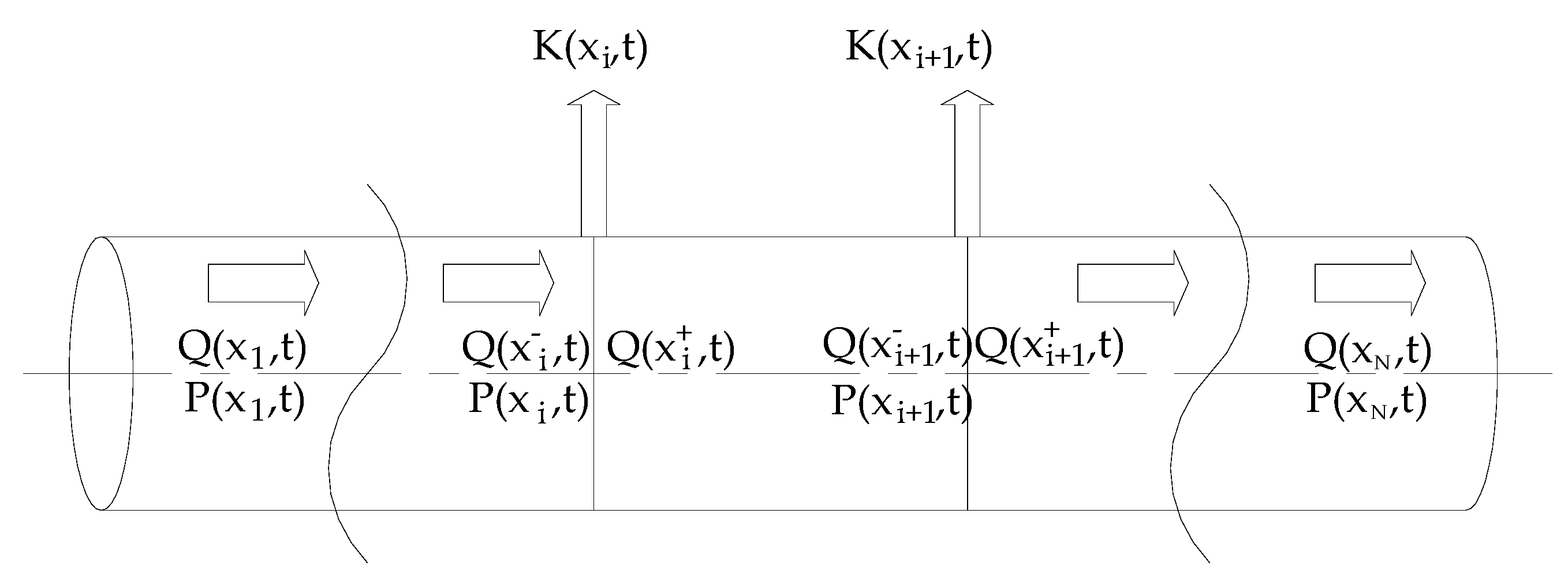
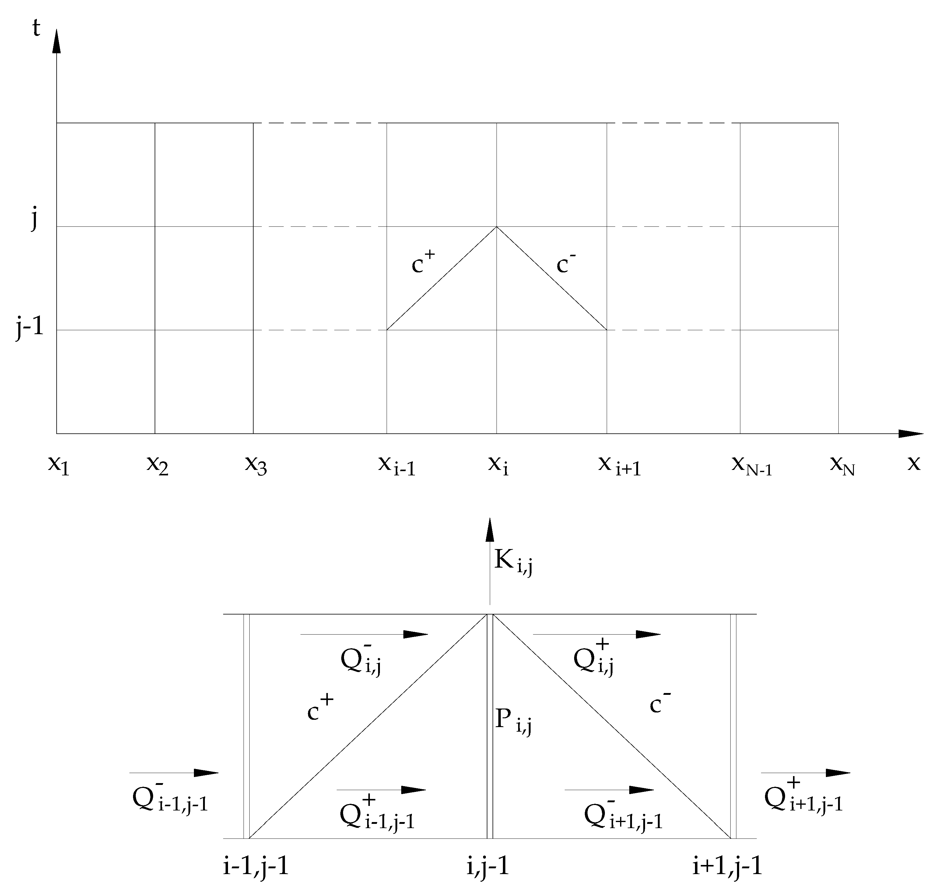
Since EKF can only be applied to the form of discrete time and discrete space for state estimation, it is necessary to discretize the pipeline length and leakage rate. The basic idea is presented below. First, the pipeline model is divided into segments, and the position coordinates on each segment point are , , …, , , …, , . Assume the leakage happens at points , …, , , …, , segments. At time t, the pressure, flow, and virtual leakage rate at point are represented as , , and , respectively. The actual leaking pipeline and the virtual multi-point leaking pipeline are shown in Figure 1 and Figure 2, respectively.
The method of a characteristic line is used to solve the basic control equation of natural gas flow. Combining the above ideas, the leakage is virtually distributed at segment points, as shown in Figure 3, and the corresponding discrete equations can be obtained as [72,73]
where i is the subscript to represent a segment , j is the subscript to represent time , is mass flow before the leakage point at the segment at time , kg/s, is mass flow after the leakage point, kg/s, is pressure before the leakage point, Pa, is pressure after the leakage point, Pa, is the cross-sectional area of pipe, m2, is the speed of sound, m/s, is pipe diameter, m, and is the hydraulic friction coefficient.
Since the leakage occurs in the vertical direction, it can be assumed that the momentum change caused by the leakage in the horizontal direction can be ignored. According to the principle of mass conservation, the boundary conditions at the leakage point can be given as
Among them, i = 1, 2, …, N; j = 1, 2, …, , and represent the mass flow and pressure at time at position (before the leakage point), namely and . In the same way, , , , , and .
The EKF-based method proposed in this paper assumes that the leakage rate at each segment point is constant in time [74,75,76,77,78], namely,
Equations (1)–(5) are based on the basic idea of filter estimation, and the discretized pipeline transient flow model including virtual multi-point leakage can now be established, as follows.
To make the virtual leakage rate a component of the state variables in the above model, Equations (3) and (4) are substituted into Equations (1) and (2) to give
Equations (5)–(7) constitute a nonlinear implicit system with the following variables: pressure at each segment point , the flow rate to the left of each segment point , and the virtual leakage rate at each segment point. These variables constitute a dimensional state vector:
Therefore, the nonlinear implicit system can be expressed as
where and is the boundary condition of P and Q in this system.
3. State Estimation by EKF
To use the EKF method, the system needs to be linearized first. Assuming that the optimal estimate of is , the corresponding state Equation can be written according to the EKF,
where , is the transition matrix that can be obtained in the linearization process, and is the system noise. The corresponding measurement Equation can be written as
where is the measurement matrix and is the measurement noise. Both system noise and measurement noise are assumed to be zero-mean Gaussian white noise in the Kalman filter.
Let represent the prior estimate of the state variables at time obtained using the optimal estimate at time . Let represent the optimal estimate of the state variables at time . Correspondingly:
In the following discussion, is the variance matrix of the prior estimation error, is the optimal estimation variance matrix ( is known), is the Kalman gain, and is the variance matrix of the measurement noise. The steps of applying EKF to estimate state variables are as follows [79,80]:
- With the initial value , linearize the Equations near and obtain the transfer matrix ;
- Solve the nonlinear Equations (5)–(7), as , and can be computed and obtained: ; ;
- Use the following formula to compute the Kalman gain: ;
- Obtain the optimal estimate by measuring the valueobtain the optimal estimated variance matrix at time jobtain the optimal estimate by measuring the valueand obtain the optimal estimated variance matrix at time
- Go back to step 2 and calculate the optimal estimate of the moment . From the above computation, we can obtain the optimal estimation of the state vector .
4. Calculating the Actual Leakage Rate and Location
The above estimated state vectors include the pressure at each segment point , the flow to the left of each segment point , and the virtual leakage rate at each segment point. To obtain the real leakage rate and the location, the idea of an equivalent system is used. That is, the virtual multi-point leakage pipeline should have the same initial conditions and boundary conditions as the actual pipeline. The pipeline flow loss and pressure drop caused by both of them should be the same. The computation formula of the actual leakage rate and leakage location of the actual pipeline [73] can be defined as follows.
Using the virtual leakage rate at each segment point and the known , combined with Equation (13), the actual leakage rate and leakage location of the actual pipeline can be obtained.
5. A Simulation Example
The model is first verified with a simulation example. In this example, the process noise and measurement noise of this simulated gas pipeline are assumed to be Gaussian white noise. The specific parameters are:
The boundary conditions are: .
Generally, the length of each segment needs to be slightly larger than or equal to the distance that sound travels within one sampling period of the sensor ( ). If the segment length is shorter than that distance, then it is possible to miss the data. If the segment length is too long, then the precision may be reduced. In this example, the sampling frequencies f of pressure sensors are assumed to be 1 Hz, therefore . Therefore, the pipeline is divided into segments by the characteristic line method, namely N = 31.
It is assumed that the leakage occurs at 500 s, and the leakage point is 4 km away from the starting pressure sensor. To simulate a slow small leakage, set the leakage rate to be 4% of the total flow rate, i.e., 0.1 kg/s.
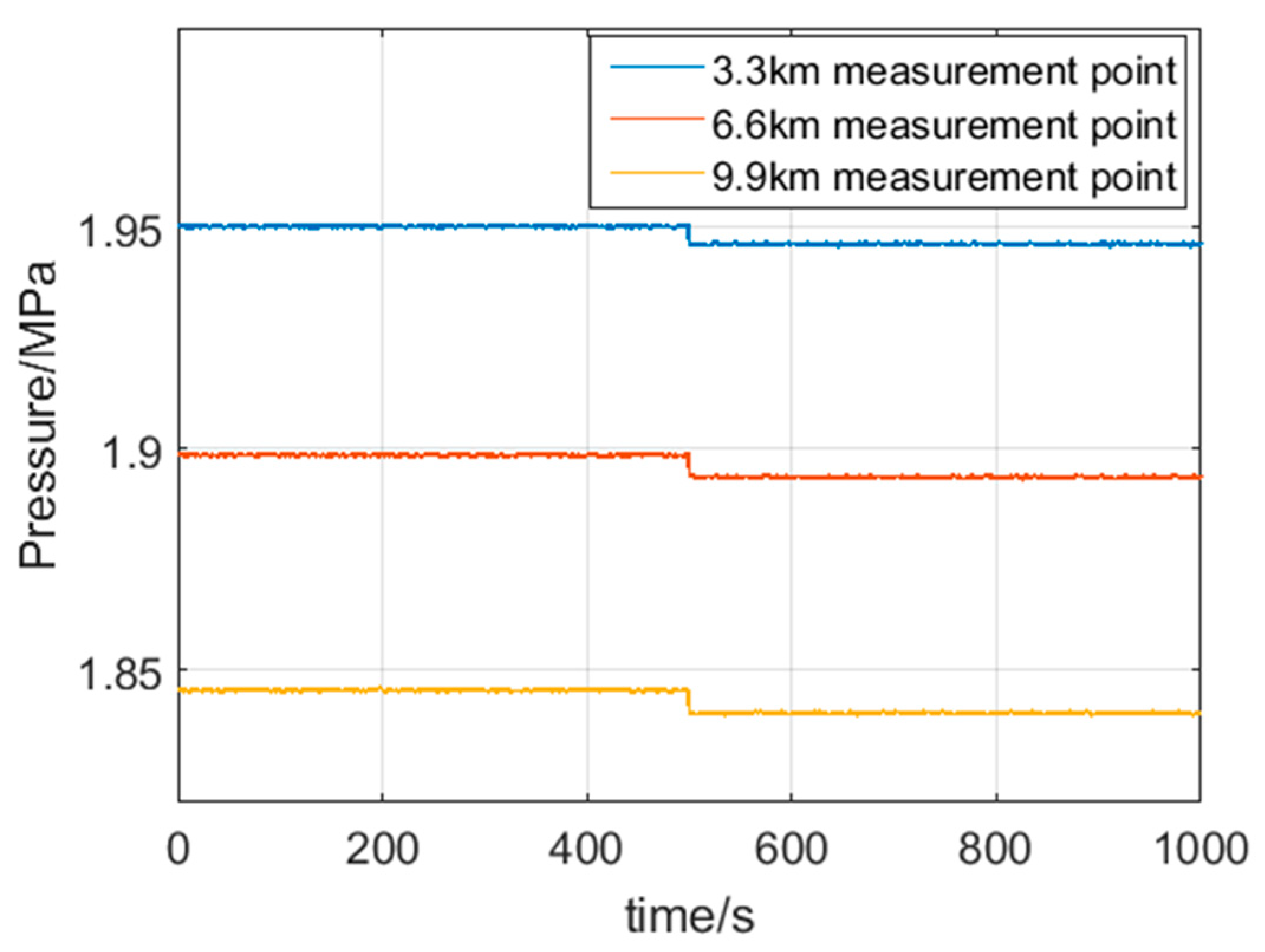
In this simulation example, there are three pressure observation points at 3.3 km, 6.6 km, and 9.9 km, namely , , and , respectively.
The state vector is:
Therefore, in this simulation example, the measurement matrix is a matrix of , , and . The rest of the elements are set as 0.
The initial condition is:
Among them:
P11,0 = 1,949, 679 Pa, P21,0 = 1,898,024 Pa, P31,0 = 1,844,923 Pa
is a 91 × 91 diagonal matrix, where is a diagonal matrix. Here, the assumptions are:
The covariance of process noise and measurement noise is known. It is assumed that it does not vary with the state variable [12].
where is the noise variance of pressure, and are the variance of the noise of flow and leakage rate, respectively. is the measurement noise variance of pressure. Here, the assumptions are: , , and .
Based on the steady pressure distribution along the pipeline, the steady state pressure values at the three pressure measurement points before and after leakage are calculated, and the Gaussian white noise is added to construct the pressure simulation data at the pressure measurement points, as shown in Figure 4.
By using the simulation data shown in Figure 4 as the measurement data, and using the iterative procedure based on the calculation steps described above, the estimated leakage rate and leakage location by EKF are obtained, as shown in Figure 5 and Figure 6.
As can be seen in Figure 5, the design leakage rate has a step-wise change in flow rate representing a leak that commences at 500 s into the simulation, and the leakage rate is 4% of flow, i.e., 0.1 kg/s. It can be seen that the estimated leakage rate curve is basically consistent with the designed leakage rate curve, indicating that the proposed method based on EKF can detect the leakage and estimate the leakage rate accurately.
It is clear from Figure 6 that the design leakage location is 4 km downstream in the pipeline, and the curve is the estimated leakage location of the EKF. It can be seen from the figure that the two curves are also basically consistent, and the results show that the proposed method can locate the leakage position.
6. A Physical Experiment Case Study
Due to the flammable and explosive nature of natural gas, it is nearly impossible to carry out leakage rate measurement experiments using real natural gas in a pipeline. In this paper, an experimental platform was built, and compressed air was used instead of natural gas in the experiment for safety reasons.
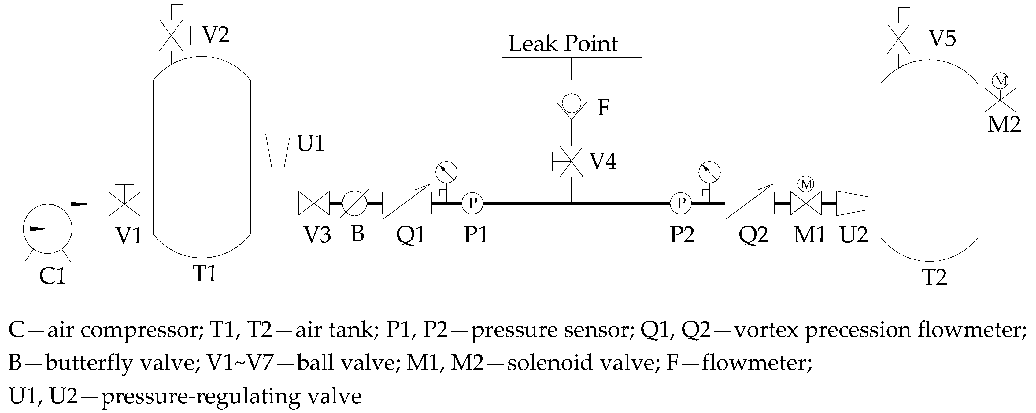
The system setup, displaying the layout of the gas leakage experimental platform, is shown in Figure 7. The platform is mainly composed of pipeline sections, a compressor, and air tanks. The compressor is a belt piston machine, with a 7.5 kW rated power, 800 L/min displacement, and 1.25 MPa working pressure. The dimensions of the cylindrical air tanks are 1 × 2.4 m (diameter × height). The weight of the air tank is 515 kg. There is one location where a leak can be simulated, named leak point in Figure 7. A leakage can be simulated by opening valve V4, and a flowmeter is set to measure the leakage rate. There are two pressure sensors (P1, P2). The specific parameters of the experimental pipeline are:
L (the length between P1 and P2) = 9 m, D (inner diameter) = 0.253 m, c = 300 m/s.
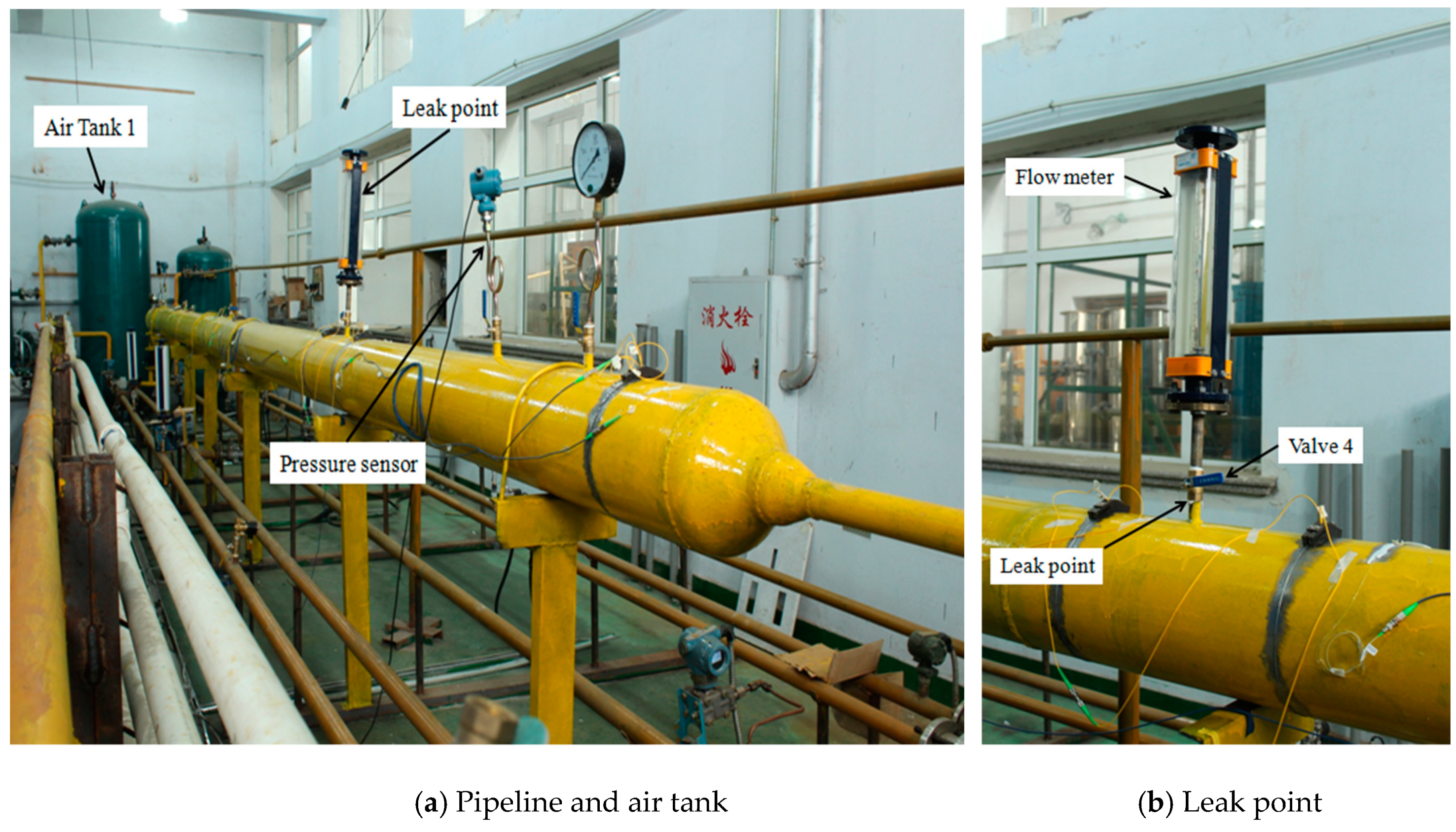
The photos of the platform are shown in Figure 8.
The sampling frequencies f of pressure sensors and flow sensors are 1000 Hz, so:
The pipe is divided into segments, where N = 31.
Referring to Figure 7, the specific steps of the experiment are as follows.
- In order to simulate the actual natural gas pipelines, an air compressor is used to pressurize tank T1.
- Once a stable pressure is achieved, the valve M1 is opened to form the flow from T1 to T2.
- Adjusting the pressure of the gas storage tank and the opening of the butterfly valve B to maintain starting and ending pressures in the pipeline to be 800 and 750 kPa, respectively. At this point, the flow rate at the beginning of the pipeline is 132 kg/h and all the sensors begin to collect data.
- After 80 s, the ball valve V4 is open to a certain degree to allow a leak at leak point 1.
After 20 s, V4 is closed to stop the leak.
The state vector is:
The initial condition is:
Among them,
P1,0 = 800 kPa, P31,0 = 750 kPa
There are three observation points of starting pressure, flow, and terminal pressure in this experiment. Therefore, the matrix H has the dimension of , where , , and the remainder of elements were 0.
The measurement noise covariance was estimated by the data collected in the experiment. The setting of process noise was similar to the simulation example.
The computational steps in the simulation example were repeated to obtain the estimated leakage rate and leakage location with the EKF, as shown in Figure 9 and Figure 10.
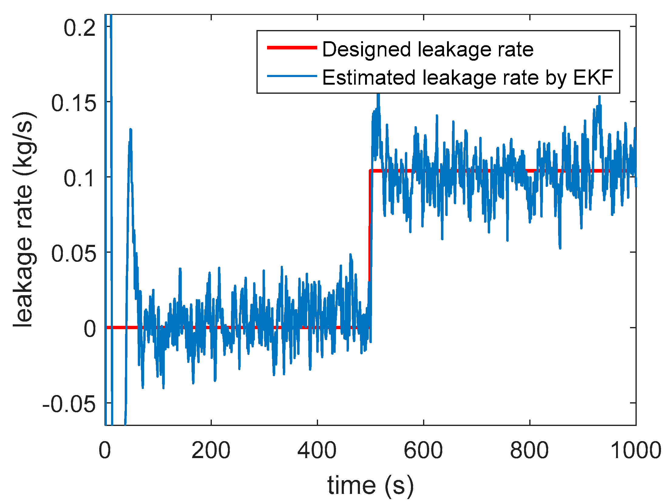
As can be seen from Figure 9, the estimated leakage rate increased between 80 and 100 s and then declined thereafter. This is consistent with the experimental procedure where leakage commences at 80 s through the opening of the ball valve. By 100 s, the leak has stopped and the leak was reduced to zero. It can be seen from the analysis that the change of the estimated leakage rate is consistent with the change of the actual leakage rate. Since the leakage state cannot be maintained under experimental conditions, the estimation of the leakage rate is affected. It can be assumed that if the leakage was not stopped during the experiment and the leakage was kept to a steady state, the estimated leakage rate of EKF would maintain a relatively stable state after rising to the highest point, which is similar to the result in Figure 6. In the experiment, the maximum value of the leakage rate read by the rotor flowmeter at the leakage point 1 was about 6.8 kg/h, and the highest point of the estimated curve of leakage rate was about 6.2 kg/h. The absolute error was 0.6 kg/h and the relative error was 8.8%. Experimental results and simulation results show that the method based on EKF is feasible to detect the leakage of a natural gas pipeline and estimate the leakage rate.
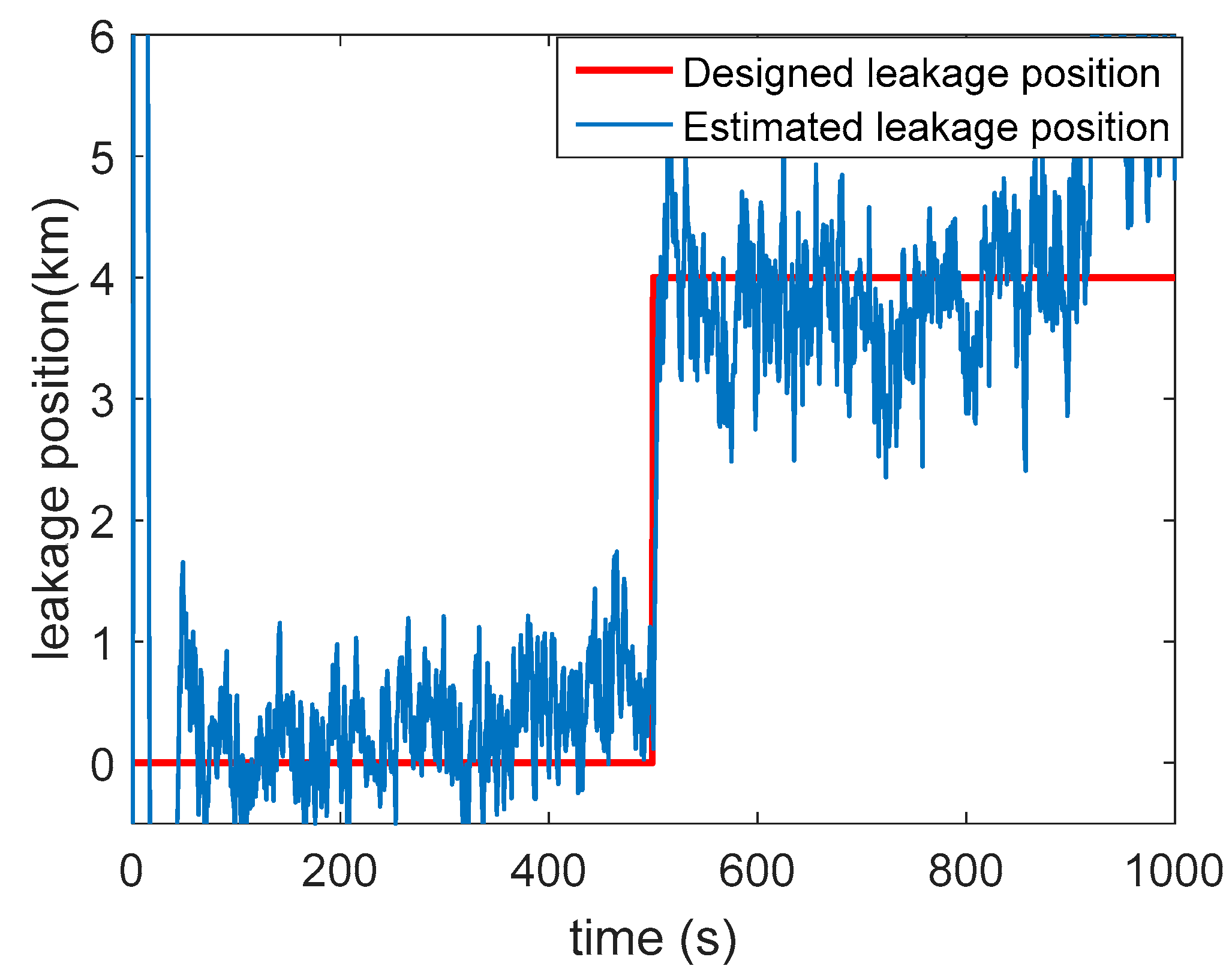
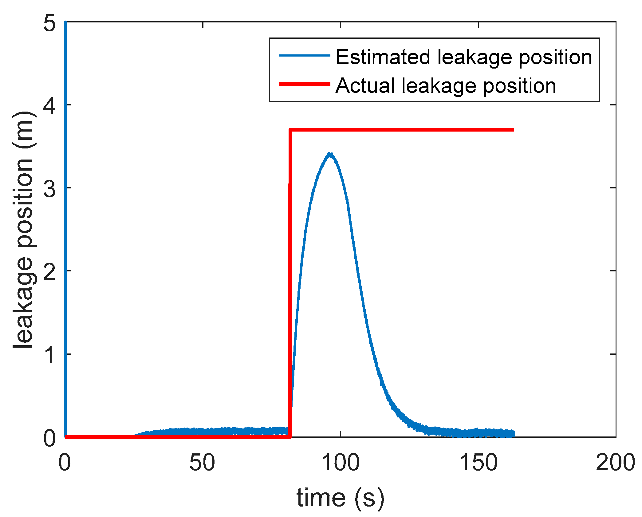
The red line in Figure 10 represents the actual leakage location, and the blue line represents the estimated curve of the leakage location. It is not difficult to explain why the estimated curve of the leakage position rises and then falls, according to the change of the estimated value of leakage rate and Equation (13). The actual pipeline leakage point 1 is 3.9 m away from the pipeline starting point pressure sensor P1, while the peak of the estimated leakage position curve is about 3.3 m. The absolute error is 0.6 m. As the distance between pressure sensor P1 and P2 is 9 m, the relative error is 6.7%. It is conjectured that if the leakage was not stopped, the positioning accuracy would be further improved. The result of the experiment shows that the proposed method based on EKF is feasible to locate leakages in natural gas pipelines.
7. Conclusion and Future Work
This paper introduces a method of natural gas pipeline leak detection based on the extended Kalman filter (EKF). The change of flow state in an actual pipeline operation is usually random and easily affected by all kinds of interferences. Therefore, it is difficult to reflect the real-time state of flow by the transient flow real-time model method directly. This paper proposes a time-varying real-time EKF method for pipeline leak detection. In applying the approach to simulated and laboratory case studies, this paper has shown that the separate treatment of system and measurement noise inherent within EKF means that the proposed approach has low sensitivity to random noise, and good capability for accurately estimating leakage rate and location. The results of simulation and experiment show that the method is sensitive to small leakages of a pipeline and the estimation of leakage rate and location are accurate.
As the foundational work on an algorithm and experimental study, there are several limitations which we would like to address in future work. Firstly, the algorithm is only applied to long straight pipeline but not a pipeline network with complex topology. Secondly, the experimental study is verified on a lab testbed that is smaller than typical real-world gas pipelines. It will be critical to work with gas companies to experiment with real gas pipelines. Thirdly, while the probability of a multi-point leakage is much lower than that of a single-point leakage, it is still useful to conduct research in detecting leakage in more complex cases.
Author Contributions
Q.H. derived the algorithms, led the experiments and wrote the paper. W.Z. revised and proofread the paper.
Funding
This research was funded by Scientific Research Project of Harbin University of Commerce (No. 17XN013) entitled “Research about detection and location of natural gas pipeline leakages based on Kalman filter and Fiber sensing,” the Doctoral Research Project of Harbin University of Commerce (No. 2016BS19), and National Natural Science Foundation of China (No. 51808092).
Conflicts of Interest
The authors declare no conflicts of interest.
References
- Montiel, H.; Vilchez, J.; Casal, J.; Arnaldos, J. Mathematical modelling of accidental gas releases. J. Hazard. Mater. 1998, 59, 211–233. [Google Scholar] [CrossRef]
- Kostowski, W.J.; Skorek, J. Real gas flow simulation in damaged distribution pipelines. Energy 2012, 45, 481–488. [Google Scholar] [CrossRef]
- Bariha, N.; Mishra, I.M.; Srivastava, V.C. Hazard analysis of failure of natural gas and petroleum gas pipelines. J. Loss Prev. Process Ind. 2016, 40, 217–226. [Google Scholar] [CrossRef]
- Damavandi, M.Y.; Kiaei, I.; Sheikh-El-Eslami, M.K.; Seifi, H.; Sheikh-El-Eslami, M.K. New approach to gas network modeling in unit commitment. Energy 2011, 36, 6243–6250. [Google Scholar] [CrossRef]
- Fu, Z.M.; Huang, J.Y.; Fu, M. Quantitative analysis of thermal radiation damaging effects caused by liquid or gaseous hydrocarbon fires. China Saf. Sci. J. 2008, 18, 29–36. [Google Scholar]
- Szente, V.; Vad, J.A. Semi-empirical model for characterisation of flow coefficient for pneumatic solenoid valves. Periodica Polytech. Mech. Eng. 2004, 47, 131–142. [Google Scholar]
- Demissie, A.; Zhu, W.; Belachew, C.T. A multi-objective optimization model for gas pipeline operations. Comput. Chem. Eng. 2017, 100, 94–103. [Google Scholar] [CrossRef] [Green Version]
- Zeng, X.; Dong, F.-F.; Xie, X.-D.; Du, G.-F. A new analytical method of strain and deformation of pipeline under fault movement. Int. J. Press. Vessels Pip. 2019, 172, 199–211. [Google Scholar] [CrossRef]
- Zhu, J.; Ho, S.C.M.; Patil, D.; Wang, N.; Hirsch, R.; Song, G. Underwater pipeline impact localization using piezoceramic transducers. Smart Mater. Struct. 2017, 26, 107002. [Google Scholar] [CrossRef] [Green Version]
- Jiang, T.; Ren, L.; Jia, Z.; Li, D.; Li, H. Application of FBG Based Sensor in Pipeline Safety Monitoring. Appl. Sci. 2017, 7, 540–551. [Google Scholar] [CrossRef]
- Siswantoro, N.; Doğan, A.; Priyanta, D.; Zaman, M.B.; Semin, S. Possibility of Piezoelectric Sensor to Monitor Onshore Pipeline in Real Time Monitoring. Int. J. Mar. Eng. Innov. Res. 2019, 3, 199–211. [Google Scholar] [CrossRef]
- Von Fischer, J.C.; Cooley, D.; Chamberlain, S.; Gaylord, A.; Griebenow, C.J.; Hamburg, S.P.; Salo, J.; Schumacher, R.; Theobald, D.; Ham, J. Rapid, vehicle-based identification of location and magnitude of urban natural gas pipeline leaks. Environ. Sci. Technol. 2017, 51, 4091–4099. [Google Scholar] [CrossRef] [PubMed]
- Pham, H.Q.; Tran, B.V.; Doan, D.T.; Le, V.S.; Pham, Q.N.; Kim, K.; Kim, C.; Terki, F.; Tran, Q.H. Highly Sensitive Planar Hall Magnetoresistive Sensor for Magnetic Flux Leakage Pipeline Inspection. IEEE Trans. Magn. 2018, 54, 1–5. [Google Scholar] [CrossRef]
- Chen, Q.; Shen, G.; Jiang, J.; Diao, X.; Wang, Z.; Ni, L.; Dou, Z. Effect of rubber washers on leak location for assembled pressurized liquid pipeline based on negative pressure wave method. Process Saf. Environ. Prot. 2018, 119, 181–190. [Google Scholar] [CrossRef]
- Ge, C.; Wang, G.; Ye, H. Analysis of the smallest detectable leakage flow rate of negative pressure wave-based leak detection systems for liquid pipelines. Comput. Chem. Eng. 2008, 32, 1669–1680. [Google Scholar] [CrossRef]
- Silva, R.A.; Buiatti, C.M.; Cruz, S.L.; Pereira, J.A.F.R. Pressure wave behavior and leak detection in pipelines. Comput. Chem. Eng. 1996, 20, 491–496. [Google Scholar] [CrossRef]
- Yashiro, S.; Okabe, T.; Takeda, N. Damage identification in a holed CFRP laminate using a chirped fiber Bragg grating sensor. Compos. Sci. Technol. 2007, 67, 286–295. [Google Scholar] [CrossRef]
- Tsuda, H.; Lee, J.-R.; Guan, Y. Fatigue crack propagation monitoring of stainless steel using fiber Bragg grating ultrasound sensors. Smart Mater. Struct. 2006, 15, 1429. [Google Scholar] [CrossRef]
- Ali, S.; Bin Qaisar, S.; Saeed, H.; Khan, M.F.; Naeem, M.; Anpalagan, A. Network Challenges for Cyber Physical Systems with Tiny Wireless Devices: A Case Study on Reliable Pipeline Condition Monitoring. Sensors 2015, 15, 7172–7205. [Google Scholar] [CrossRef] [Green Version]
- Huo, L.; Li, C.; Jiang, T.; Li, H.-N. Feasibility Study of Steel Bar Corrosion Monitoring Using a Piezoceramic Transducer Enabled Time Reversal Method. Appl. Sci. 2018, 8, 2304–2317. [Google Scholar] [CrossRef]
- Soojin, C.; Yun, C.; Lynch, J.P.; Zimmerman, A.T. Smart Wireless Sensor Technology for Structural Health Monitoring of Civil Structures. Steel Struct. 2008, 8, 267–275. [Google Scholar]
- Soojin, C.; Lynch, J.P.; Lee, J.J. Development of an Automated Wireless Tension Force Estimation System for Cable-stayed Bridges. J. Intell. Mater. Syst. Struct. 2009, 21, 361–376. [Google Scholar]
- Jang, S.; Jo, H.; Cho, S.; Mechitov, K.; Rice, J.A.; Sim, S.-H.; Jung, H.-J.; Yun, C.-B.; Spencer, B.F.J.; Agha, G. Structural health monitoring of a cable-stayed bridge using smart sensor technology: Deployment and evaluation. Smart Struct. Syst. 2010, 6, 439–459. [Google Scholar] [CrossRef]
- Song, G.; Wang, C.; Wang, B. Structural Health Monitoring (SHM) of Civil Structures. Appl. Sci. 2018, 7, 789–791. [Google Scholar] [CrossRef]
- Zhang, X.; Zhang, L.; Liu, L.; Huo, L. Prestress Monitoring of a Steel Strand in an Anchorage Connection Using Piezoceramic Transducers and Time Reversal Method. Sensors 2018, 18, 4018–4037. [Google Scholar] [CrossRef] [PubMed]
- Mitra, M.; Gopalakrishnan, S. Guided wave based structural health monitoring: A review. Smart Mater. Struct. 2016, 25, 053001. [Google Scholar] [CrossRef]
- Kong, Q.; Robert, R.H.; Silva, P.; Mo, Y.L. Cyclic Crack Monitoring of a Reinforced Concrete Column under Simulated Pseudo-Dynamic Loading Using Piezoceramic-Based Smart Aggregates. Appl. Sci. 2016, 6, 341–354. [Google Scholar] [CrossRef]
- Wang, Y.; Zhu, X.; Hao, H.; Ou, J. Guided wave propagation and spectral element method for debonding damage assessment in RC structures. J. Sound Vib. 2009, 324, 751–772. [Google Scholar] [CrossRef]
- Lu, G.; Li, Y.; Wang, T.; Xiao, H.; Xiao, H. A multi-delay-and-sum imaging algorithm for damage detection using piezoceramic transducers. J. Intell. Mater. Syst. Struct. 2017, 28, 1150–1159. [Google Scholar] [CrossRef]
- Yang, J.; Choi, J.; Hwang, S.; An, Y.-K.; Sohn, H. A reference-free micro defect visualization using pulse laser scanning thermography and image processing. Meas. Sci. Technol. 2016, 27, 085601–085610. [Google Scholar] [CrossRef]
- Hou, J.; Wang, P.; Jing, T.; Jankowski, Ł. Experimental Study for Damage Identification of Storage Tanks by Adding Virtual Masses. Sensors 2019, 19, 220–236. [Google Scholar] [CrossRef] [PubMed]
- Kim, N.; Jang, K.; An, Y.-K. Self-Sensing Nonlinear Ultrasonic Fatigue Crack Detection under Temperature Variation. Sensors 2018, 18, 2527–2541. [Google Scholar] [CrossRef] [PubMed]
- Yang, Y.; Liu, H.; Annamdas, V.G.M.; Soh, C.K. Monitoring damage propagation using PZT impedance transducers. Smart Mater. Struct. 2009, 18, 045003. [Google Scholar] [CrossRef]
- John, S.; Sirohi, J.; Wang, G.; Wereley, N.M. Comparison of piezoelectric, magnetostrictive, and electrostrictive hybrid hydraulic actuators. J. Intell. Mater. Syst. Struct. 2007, 18, 1035–1048. [Google Scholar] [CrossRef]
- An, Y.-K.; Shen, Z.; Wu, Z. Stripe-PZT Sensor-Based Baseline-Free Crack Diagnosis in a Structure with a Welded Stiffener. Sensors 2016, 16, 1511–1529. [Google Scholar] [CrossRef] [PubMed]
- Wang, F.; Ho, S.C.M.; Huo, L.; Song, G. A novel fractal contact-electromechanical impedance model for quantitative monitoring of bolted joint looseness. IEEE Access 2018, 6, 40212–40220. [Google Scholar] [CrossRef]
- Kong, Q.; Fan, S.; Bai, X.; Mo, Y.L.; Song, G. A novel embeddable spherical smart aggregate for structural health monitoring: Part I. Fabrication and electrical characterization. Smart Mater. Struct. 2017, 26, 095050. [Google Scholar] [CrossRef]
- Kong, Q.; Fan, S.; Mo, Y.L.; Song, G. A novel embeddable spherical smart aggregate for structural health monitoring: Part II. Numerical and experimental verifications. Smart Mater. Struct. 2017, 26, 095051. [Google Scholar] [CrossRef]
- Dumoulin, C.; Deraemaeker, A. Real-time fast ultrasonic monitoring of concrete cracking using embedded piezoelectric transducers. Smart Mater. Struct. 2017, 26, 104006. [Google Scholar] [CrossRef]
- Ghimire, M.; Wang, C.; Dixon, K.; Serrato, M. In situ monitoring of prestressed concrete using embedded fiber loop ringdown strain sensor. Measurement 2018, 124, 224–232. [Google Scholar] [CrossRef]
- Tejedor, J.; Macias-Guarasa, J.; Martins, H.F.; Piote, D.; Pastor-Graells, J.; Martin-Lopez, S.; Corredera, P.; Gonzalez-Herraez, M. A Novel Fiber Optic Based Surveillance System for Prevention of Pipeline Integrity Threats. Sensors 2017, 17, 355–373. [Google Scholar] [CrossRef] [PubMed]
- Kong, X.; Ho, S.C.M.; Song, G.; Cai, C.S. Scour Monitoring System Using Fiber Bragg Grating Sensors and Water-Swellable Polymers. J. Bridg. Eng. 2017, 22, 04017029–04017039. [Google Scholar] [CrossRef]
- Meng, L.; Wang, L.; Hou, Y. Development of Large-Strain Macrobend Optical-Fiber Sensor with Helical-Bending Structure for Pavement Monitoring Application. J. Aerosp. Eng. 2019, 32, 04019021–04019030. [Google Scholar] [CrossRef]
- Zhang, G.; Zhu, J.; Song, Y.; Peng, C.; Song, G. A Time Reversal Based Pipeline Leakage Localization Method with the Adjustable Resolution. IEEE Access 2018, 6, 26993–27000. [Google Scholar] [CrossRef]
- Chen, B.; Hei, C.; Luo, M.; Ho, M.S.C.; Song, G.; Chuang, H. Pipeline two-dimensional impact location determination using time of arrival with instant phase (TOAIP) with piezoceramic transducer array. Smart Mater. Struct. 2018, 27, 105003. [Google Scholar] [CrossRef]
- Du, G.; Kong, Q.; Zhou, H.; Gu, H. Multiple Cracks Detection in Pipeline Using Damage Index Matrix Based on Piezoceramic Transducer-Enabled Stress Wave Propagation. Sensors 2017, 17, 1812–1822. [Google Scholar] [CrossRef] [PubMed]
- Ren, L.; Jiang, T.; Jia, Z.-G.; Li, D.-S.; Yuan, C.-L.; Li, H.-N. Pipeline corrosion and leakage monitoring based on the distributed optical fiber sensing technology. Measurement 2018, 122, 57–65. [Google Scholar] [CrossRef]
- Zhao, X.; Li, W.; Zhou, L.; Song, G.; Ba, Q.; Ho, S.C.M.; Ou, J. Application of support vector machine for pattern classification of active thermometry based pipeline scour monitoring. Struct. Control Health Monit. 2015, 22, 903–918. [Google Scholar] [CrossRef]
- Jia, Z.; Ren, L.; Li, H.; Wu, W.; Jiang, T. Performance Study of FBG Hoop Strain Sensor for Pipeline Leak Detection and Localization. J. Aerosp. Eng. 2018, 31, 04018050–04018059. [Google Scholar] [CrossRef]
- Hou, Q.; Jiao, W.; Ren, L.; Cao, H.; Song, G. Experimental study of leakage detection of natural gas pipeline using FBG based strain sensor and least square support vector machine. J. Loss Prev. Process. Ind. 2014, 32, 144–151. [Google Scholar] [CrossRef]
- Zhu, J.; Ren, L.; Ho, S.C.M.; Jia, Z.; Song, G. Gas pipeline leakage detection based on PZT sensors. Smart Mater. Struct. 2017, 26, 025022. [Google Scholar] [CrossRef]
- Jia, Z.G.; Ren, L.; Li, H.N.; Ho, S.; Song, G. Experimental study of pipeline leak detection based on hoop strain measurement. Struct. Control Health Monit. 2015, 22, 799–812. [Google Scholar] [CrossRef]
- Ren, L.; Jia, Z.-G.; Li, H.-N.; Song, G. Design and experimental study on FBG hoop-strain sensor in pipeline monitoring. Opt. Fiber Technol. 2014, 20, 15–23. [Google Scholar] [CrossRef]
- Hou, Q.; Ren, L.; Jiao, W.; Zou, P.; Song, G. An Improved Negative Pressure Wave Method for Natural Gas Pipeline Leak Location Using FBG Based Strain Sensor and Wavelet Transform. Math. Probl. Eng. 2013, 2013, 1–8. [Google Scholar] [CrossRef] [Green Version]
- Wang, F.; Huo, L.; Song, G. A piezoelectric active sensing method for quantitative monitoring of bolt loosening using energy dissipation caused by tangential damping based on the fractal contact theory. Smart Mater. Struct. 2017, 27, 015023. [Google Scholar] [CrossRef]
- Huynh, T.-C.; Dang, N.-L.; Kim, J.-T. Preload Monitoring in Bolted Connection Using Piezoelectric-Based Smart Interface. Sensors 2018, 18, 2766–2785. [Google Scholar] [CrossRef] [PubMed]
- Yin, H.; Wang, T.; Yang, D.; Liu, S.; Shao, J.; Li, Y. A Smart Washer for Bolt Looseness Monitoring Based on Piezoelectric Active Sensing Method. Appl. Sci. 2016, 6, 320–329. [Google Scholar] [CrossRef]
- Du, G.F.; Kong, Q.Z.; Wu, F.H.; Ruan, J.; Song, G. An experimental feasibility study of pipeline corrosion pit detection using a piezoceramic time reversal mirror. Smart Mater. Struct. 2016, 25, 037002. [Google Scholar] [CrossRef]
- Peng, J.; Hu, S.; Zhang, J.; Cai, C.; Li, L.-Y. Influence of cracks on chloride diffusivity in concrete: A five-phase mesoscale model approach. Constr. Build. Mater. 2019, 197, 587–596. [Google Scholar] [CrossRef]
- Li, X.; Bai, Y.; Su, C.; Li, M. Effect of interaction between corrosion defects on failure pressure of thin wall steel pipeline. Int. J. Press. Vessels Pip. 2016, 138, 8–18. [Google Scholar] [CrossRef]
- Khante, S.N.; Jain, N. Erosion Identification and Assessment of a Steel Pipeline Using EMI Technique; Springer Science and Business Media LLC: Berlin/Heidelberg, Germany, 2018; pp. 347–355. [Google Scholar]
- Du, G.; Kong, Q.; Lai, T.; Song, G. Feasibility Study on Crack Detection of Pipelines Using Piezoceramic Transducers. Int. J. Distrib. Sens. Netw. 2013. [Google Scholar] [CrossRef]
- Camerini, C.; Rebello, J.M.A.; Braga, L.; Santos, R.; Chady, T.; Psuj, G.; Pereira, G. In-Line Inspection Tool with Eddy Current Instrumentation for Fatigue Crack Detection. Sensors 2018, 18, 2161–2172. [Google Scholar] [CrossRef] [PubMed]
- Xu, Y.; Luo, M.; Liu, Q.; Du, G.; Song, G. PZT transducer array enabled pipeline defect locating based on time-reversal method and matching pursuit de-noising. Smart Mater. Struct. 2019, 28. [Google Scholar] [CrossRef]
- Evgeniou, T.; Pontil, M.; Poggio, T. Regularization Networks and Support Vector Machines. Adv. Comput. Math. 2000, 13, 1–50. [Google Scholar] [CrossRef]
- Geiger, G.; Bollermann, B.; Tetzner, R. Leak monitoring of an ethylene gas pipeline. In Proceedings of the PSIG Annual Meeting, Palm Springs, CA, USA, 20–22 October 2004. [Google Scholar]
- Julier, S.J.; Uhlmann, J.K. New extension of the Kalman filter to nonlinear systems. In Proceedings of the AeroSense ’97, Orlando, FL, USA, 20–25 April 1997; pp. 182–193. [Google Scholar]
- Xie, L.; Zhou, Z.; Zhao, L.; Wan, C.; Tang, H.; Xue, S. Parameter Identification for Structural Health Monitoring with Extended Kalman Filter Considering Integration and Noise Effect. Appl. Sci. 2018, 8, 2480–2498. [Google Scholar] [CrossRef]
- Hao, Y.; Xu, A.; Sui, X.; Wang, Y. A Modified Extended Kalman Filter for a Two-Antenna GPS/INS Vehicular Navigation System. Sensors 2018, 18, 3809–3830. [Google Scholar] [CrossRef] [PubMed]
- Pointon, H.A.G.; McLoughlin, B.J.; Matthews, C.; Bezombes, F.A. Towards a Model Based Sensor Measurement Variance Input for Extended Kalman Filter State Estimation. Drones 2019, 3, 19–37. [Google Scholar] [CrossRef]
- Ko, N.Y.; Youn, W.; Choi, I.H.; Song, G.; Kim, T.S. Features of Invariant Extended Kalman Filter Applied to Unmanned Aerial Vehicle Navigation. Sensors 2018, 18, 2855–2880. [Google Scholar] [CrossRef] [PubMed]
- Verde, C. Leakage location in pipelines by minimal order nonlinear observer. In Proceedings of the 2001 American Control Conference (Cat. No.01CH37148), Arlington, VA, USA, 25–27 June 2001; pp. 1733–1738. [Google Scholar]
- Xiao, M.L.; Zhang, Y.B. An adaptive three-stage extended Kalman filter for Nonlinear discrete-time system in presence of unknown inputs. ISA Trans. 2018, 75, 101–117. [Google Scholar] [CrossRef] [PubMed]
- Benkherouf, A. Leak detection and location in gas pipelines. Control Theory Appl. 1998, 135, 142–148. [Google Scholar] [CrossRef]
- Gomm, J. Adaptive neural network approach to on-line learning for process fault diagnosis. Trans. Inst. Meas. Control. 1998, 20, 144–152. [Google Scholar] [CrossRef]
- Cui, W. Kalman Filter Based Fault Detection and Diagnosis. Master’s Thesis, Flinders University, College of Science and Engineering, Bedford Park, Australia, 2018. [Google Scholar]
- Nguyen, L.H.; Goulet, J.-A. Anomaly detection with the Switching Kalman Filter for structural health monitoring. Struct. Control Health Monit. 2018, 25, e2136. [Google Scholar] [CrossRef]
- Sergey, A.B.; Oleg, F.L. Waves Attenuation and the Pressure Surge Method Performance. In Proceedings of the PSIG Annual Meeting, Calgary, AB, Canada, 23–26 October 2007. [Google Scholar]
- Ge, C.; Ye, H.; Wang, G.; Yang, H. A fast leak locating method based on wavelet transform. Tsinghua Sci. Technol. 2009, 14, 551–555. [Google Scholar] [CrossRef]
- Zhang, L.-B.; Qin, X.-Y.; Wang, Z.-H.; Liang, W. Designing a reliable leak detection system for West Products Pipeline. J. Loss Prev. Process Ind. 2009, 22, 981–989. [Google Scholar] [CrossRef]
Figure 1.
A real leakage in a continuous pipeline model.

Figure 2.
Virtual multi-point leakages in a discrete pipeline model.

Figure 3.
Discretization for virtual multi-point leakage in a pipeline.

Figure 4.
Pressure simulation data.

Figure 5.
Estimated leak rate using simulation data. EKF: extended Kalman filter.

Figure 6.
Estimated leak location using simulation data.

Figure 7.
The system diagram of the gas pipeline leak detection experiment testbed.

Figure 8.
Photos of the gas pipeline leak detection testbed.

Figure 9.
Estimated leakage rate using experimental data.

Figure 10.
Estimated leak position using experimental data.

© 2019 by the authors. Licensee MDPI, Basel, Switzerland. This article is an open access article distributed under the terms and conditions of the Creative Commons Attribution (CC BY) license (http://creativecommons.org/licenses/by/4.0/).
Share and Cite
MDPI and ACS Style
Hou, Q.; Zhu, W. An EKF-Based Method and Experimental Study for Small Leakage Detection and Location in Natural Gas Pipelines. Appl. Sci. 2019, 9, 3193. https://0-doi-org.brum.beds.ac.uk/10.3390/app9153193
AMA Style
Hou Q, Zhu W. An EKF-Based Method and Experimental Study for Small Leakage Detection and Location in Natural Gas Pipelines. Applied Sciences. 2019; 9(15):3193. https://0-doi-org.brum.beds.ac.uk/10.3390/app9153193
Chicago/Turabian StyleHou, Qingmin, and Weihang Zhu. 2019. "An EKF-Based Method and Experimental Study for Small Leakage Detection and Location in Natural Gas Pipelines" Applied Sciences 9, no. 15: 3193. https://0-doi-org.brum.beds.ac.uk/10.3390/app9153193
Note that from the first issue of 2016, this journal uses article numbers instead of page numbers. See further details here.