Temporal Label Walk for Community Detection and Tracking in Temporal Network

Abstract

The problem of temporal community detection is discussed in this paper. Main existing methods are either structure-based or incremental analysis. The difficulty of the former is to select a suitable time window. The latter needs to know the initial structure of networks and the changing of networks should be stable. For most real data sets, these conditions hardly prevail. A streaming method called Temporal Label Walk (TLW) is proposed in this paper, where the aforementioned restrictions are eliminated. Modularity of the snapshots is used to evaluate our method. Experiments reveal the effectiveness of TLW on temporal community detection. Compared with other static methods in real data sets, our method keeps a higher modularity with the increase of window size.

1. Introduction

The concept of community defined by Newman and Girvan is widely accepted and used [1]. Community detection is a significant task and of great value in practical applications. For sales websites, discovering consumers of different products can help website managers purchase selectively; for social networks, it will be easier to recommend friends to users if we can detect communities sharing common interests.

Research on community detection falls into two categories: static methods and temporal methods. Some classic methods such as Kernighan–Lin [2] based on graph cut and Label Propagation Algorithm (LPA) are static methods [3]. The famous Girvan and Newman (GN) algorithm [1] is also a static method. The static methods divide a network into different communities based on static graph where the relationship between nodes and edges will not change. However, increasing numbers of real data sets cannot be denoted by a static graph since edges and nodes are changing constantly. These data sets are called temporal data and the networks consisting of temporal data are called temporal networks. Temporal approaches are proposed to deal with temporal networks.

Structure-based methods and incremental analysis are the two most common methods used for community detection in a temporal network. Structure-based methods mix temporal data in the time window $\Delta t$ to a graph snapshot $G_i$ and the temporal networks can be viewed as a sequence $G_1,G_2,\dots ,G_s$ where each $G_i$ corresponds to the configuration of the graph in the ith time window [4]. For any $G_i$, it is a static network and the traditional static algorithms can be used for community detection. Meanwhile, the validation measurements used in static networks are making for temporal networks as well. If the ground-truth communities are known, Normalized Mutual Information(NMI) [5] is often used. In addition, Modularity [1] is often used while ground-truth is unknown. Determining the size of window is a problem here. If $\Delta t$ is too small, few nodes and edges are included in a snapshot. As a result, it is hard to find any community structure. On the contrary, the evolution of communities cannot be tracked if $\Delta t$ is too large.

To avoid selecting appropriate $\Delta t$, incremental analysis adds vertexes or edges to the network one by one with the transmission of temporal data stream. Much research has used incremental analysis for community detection in temporal networks. Li et al. divide communities according to permanence index [6]. Agarwal et al. maximize permanence to detect communities [7]. Guo et al. focus on local interact for community detection [8]. Ditursi et al. also use local information to find seed nodes [9]. Several pieces of incremental analysis detecting communities detection are based on label propagation [10,11]. Incremental analysis requires that community structure should be known in the beginning and the structure of networks change stably. However, community structure is unknown in most real data sets, and stability of evolution cannot be guaranteed either.

We show the form of temporal data of two methods, and the real graph sequence in Figure 1. Real data set $Students$ [12] consists of communications in a student organization. The community structure at certain nodes can obviously be observed by compressing one day’s interactions together in Figure 2.

This paper proposes a streaming method to detect and track communities without any fixed $\Delta t$. Our main contribution is two-fold:

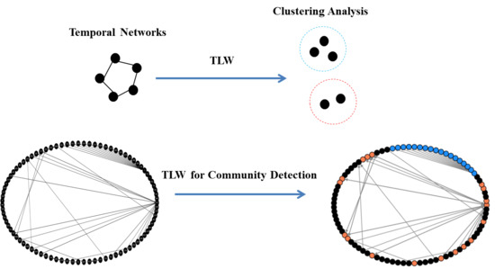
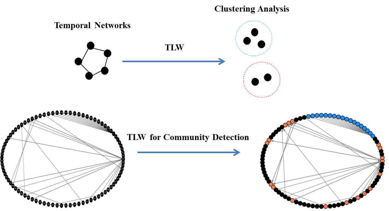
• Propose a new method called Temporal Label Walk (TLW) to detect community structure in temporal networks without time window. Our approach transforms the community detection in network into a clustering analysis in vector space where no prior about the community structure is required. TLW can also maintain modularity at a reasonable level by combining time information.
• We reveal that simply mixing temporal data to snapshots and then measuring community structure is less effective with the course of time.

2. Our Method: Temporal Label Walk (TLW)

In this section, we describe our method in three parts:

• Introduce the basic idea of our method including premise, feasibility, and process.
• Give mathematical definition of TLW.
• Measure the validation of community detection.

2.1. Basic Idea

In temporal networks, new nodes and edges are added in turn. If we use static method for community detection, we must mix the data streams in a time window to a snapshot so that each snapshot can be regarded as a static graph. In fact, there are two problems. First, how to select the time window. Snapshots in different time windows consist of different information. Second, how to mix data streams. To simply stack all edges or the weighted edges both can make result dissimilar. In fact, the intensity of interactions between two nodes depends on time in temporal networks. The result is stronger now than the past. The importance of nodes is also different due to different intensity of interactions. A natural idea is to divide communities according to the importance of nodes. Temporal walk defined by Rozenshtein and Gionis in 2016 is a good tool to measure importance of nodes in temporal networks. They use temporal walk to make an extension of static PageRank [13]. A sequence of edges $v_1\stackrel{t_0}{⟶}{v}_2\stackrel{t_1}{⟶}{v}_3\stackrel{t_2}{⟶}\cdots \stackrel{t_{j-2}}{⟶}{v}_j$ denotes a temporal walk from $v_1$ to $v_j$ where $t_i\le t_{i+1}$. Béres et al. also use temporal walk to extend static Katz centrality to temporal networks [14]. The effectiveness of temporal walks is verified in measuring the importance of nodes in temporal networks. In real networks, interactions within communities are dense but between communities they are sparse [1]. It is possible for temporal walks used to divide community structure in temporal network. However, there are some special cases that make it difficult to divide communities only by measuring the importance of nodes. Meanwhile, time is an important factor in temporal data. The information received by a node recently may be more crucial than the past. We give an example in Figure 3a,b, respectively.

The importance of nodes from different communities may be the same. Our solution is to give each node a label value then compute it by temporal walks. In this way, label values between two communities are different and thus can be divided. As to how to divide communities according to label values, we use clustering methods because each node is represented by a vector. Please note that using clustering analysis for community detection has been already considered by many researchers and it is proved to be an effective approach. Pons et al. propose a measure of similarities based on random walks to find the dense subgraphs of communities [15]. Cai et al. evaluate the performance of repeated random walks in community detection of social networks [16]. De Meo et al. add a pre-processing step in which edges are weighted according to their centrality regarding the network topology and raise the accuracy of existing algorithms on real-life data sets [17]. In addition, they combine advantages of global approaches and local methods to propose a new clustering method [18]. Rémy et al. use clustering analysis to re-identify multiple addresses belonging to a same user for bitcoin user activity [19]. We apply this idea to temporal networks and more detail is described in Section 2.2.

To summarize, we propose a streaming method for community detection in temporal networks. Label value is defined for each node and computed by temporal walk. The division of nodes is obtained by the clustering analysis of label values. The result of clustering division is the division of communities in networks.

2.2. Mathematical Definition

According to the description in Section 2.1, our method is based on two assumptions:

• Data sets are in the form of data streams,
• Interactions within communities are more frequent than those between communities.

Consider a directed graph $G_t=(V,E_t)$ where V is the set of all the nodes and $E_t$ is the set of edges at time t. We denote $T=\{t_0,t_1,\cdots ,t_i,\cdots \}$ the set of time sequence when new edges appear in the data streams. Let $X_u\left(t\right)\in {\mathbb{R}}^{\left|V\right|}$ denote the label value of node u at time t. If edge $v\to u$ appears at time $t_{i+1}\in T$, now we describe how to compute $X_u\left(t_{i+1}\right)$.

The variations of label value of u is two-fold:

• All temporal walks that end in v at $t_i$, a new temporal walk starts from v and ends in u appears at $t_{i+1}$. The variation of this new temporal walk is:

  $${\Delta }_1=X_v\left(t_i\right)·\phi (t_{i+1}-t_i),$$

  (1)

  where $\phi \left(\tau \right)=\beta ·e^{-c\tau }$ is an exponential decay function, $\beta$ is a constant and $\tau =t_{i+1}-t_i$. We use $\phi$ to represent that interactions at $t_{i+1}$ are more important than those at $t_i$.
• To maintain the timeliness of information, we define an enhancement function as another variation:

  $$E_v=\alpha ·e_v,$$

  (2)

  where $\alpha \in \mathbb{R}$ and $e_v$ is a unit vector with the vth element 1 and the rests 0. Note here v is the index of node v in set $V_t$. Label value variation of u is:

  $$\Delta =E_v+{\Delta }_1.$$

  (3)

  $\Delta$ is the variation that u only interacts with v. Denoting $S_u$ by the set of all nodes that send messages to u at $t_{i+1}$, variations of u is:

  $$\Delta =E_v+\sum _{s\in S_u}(E_s+X_s\left(t_i\right)·\phi (t_{i+1}-t_i)).$$

  (4)
  At $t_{i+1}$, the label value of u is also affected by $\phi \left(\tau \right)$. We can compute $X_u\left(t_{i+1}\right)$ by:

  $$X_u\left(t_{i+1}\right)=X_u\left(t_i\right)·\phi (t_{i+1}-t_i)+\sum _{s\in S_u}(E_s+X_s\left(t_i\right)·\phi (t_{i+1}-t_i)).$$

  (5)
  Set the label value $X_u\left(t_0\right)=e_u$. Then take the normalized vector $\frac{X_u\left(t_{i+1}\right)}{\parallel X_u\left(t_{i+1}\right){\parallel }_2}$ of $X_u\left(t_{i+1}\right)$ for the next iteration if $S_s\ne ⌀$ to avoid the rapid growth of label value. To update label value of u at $t_{i+1}$, the complete algorithm is described as follows:

  $$\begin{array}{c}Step1:X_u\left(t_0\right)=e_u,\hfill \\ Step2:X_u\left(t_{i+1}\right)=X_u\left(t_i\right)·\beta ·e^{-c(t_{i+1}-t_i)}+\sum _{v\in S_u}(\alpha ·e_v+X_v\left(t_i\right)·\beta ·e^{-c(t_{i+1}-t_i)}),\hfill \\ Step3:X_u\left(t_{i+1}\right):=\frac{X_u\left(t_{i+1}\right)}{\parallel X_u\left(t_{i+1}\right){\parallel }_2},\hfill \\ i:=i+1,\hfill \\ GotoStep2.\hfill \end{array}$$

  (6)
  Computing label value can be regarded as a mapping $f:G_i\to {\mathbb{R}}^{\left|V\right|\times \left|V\right|}$, where $G_i$ is a snapshot at $t_i$ and $f\left(G_i\right)=(X_1\left(t_i\right),X_2\left(t_i\right),\cdots ,X_{\left|V\right|}\left(t_i\right))\in {\mathbb{R}}^{\left|V\right|\times \left|V\right|}$. Community detection problem in temporal network $G_t$ can therefore be transformed to clustering analysis in high-dimensional vector space ${\mathbb{R}}^{\left|V\right|\times \left|V\right|}$.

We choose several widely used clustering methods for TLW. Affinity Propagation(AP) [20], Density-Based Spatial Clustering of Applications with Noise(DBSCAN) [21] and Mini Batch K-means are compared in the following tests. AP and DBSCAN are used when that the number of communities is unknown. If the number of clusters is known, Mini Batch K-means is adopted instead since it is much simpler [22].

2.3. Evaluation

Most real data sets are unlabeled. To evaluate the divisions of community, modularity is a mostly used measurement. Modularity is proposed by Newman [1] and defined on undirected graph as

$$Q=\frac{1}{2\left|E\right|}\sum _{v,u\in V}(A_{vu}-\frac{k_v{k}_u}{2\left|E\right|})\delta (v,u),$$

(7)

where A is the adjacency matrix of undirected graph $G=(V,E)$, $k_v\left(k_u\right)$ is the degree of nodes $v\left(u\right)$ and $\delta$ is to record whether two nodes belong to the same community:

$$\delta (v,u)=\left\{\begin{array}{cc}1,\hfill & \mathrm{if}v,u\mathrm{are}\mathrm{in}\mathrm{the}\mathrm{same}\mathrm{community},\hfill \\ 0,\hfill & \mathrm{otherwise}.\hfill \end{array}\right.$$

(8)

Here $G_t$ is a directed graph, (7) turns to

$$Q=\frac{1}{\left|E\right|}\sum _{v,u\in V}(A_{vu}-\frac{k_{outv}{k}_{inu}}{\left|E\right|})\delta (v,u),$$

(9)

where $k_{outv}$ is the out-degree of v and $k_{inu}$ is the in-degree of u.

Now make a summary of our method. TLW first updates the label value $X_u\left(t\right)$ by algorithm $\left(6\right)$, then chooses a suitable clustering method to divide vectors according to whether we know the number of communities. Nodes are divided into different communities according to the clusters which nodes belong to. Finally, we use modularity to evaluate the division.

3. Experiment and Analysis

We carry out experiments to show that our method is effective in temporal community detection. Two real data sets are used: $Students$ [12] and $Facebook$ [23]. The four-month data set $Students$ is a student community at the University of California, Irvine. Nodes represent students and edges denote message passing. The $Facebook$ data set is a three-month subset of Facebook activity in a New Orleans regional community. Codes and data sets are available online (https://github.com/Zhe-liangLiu/Temporal-Label-Walk). The experiments consist of three parts:

• Explain the importance of normalization,
• Use TLW to detect and track communities in real data sets $Students$ and $Facebook$, and the modularity of several static methods including K-clique, label propagation, and asynchronous label propagation is given.
• Discuss the effects of parameters in experiments. We put this part in Section 4.

3.1. Normalization

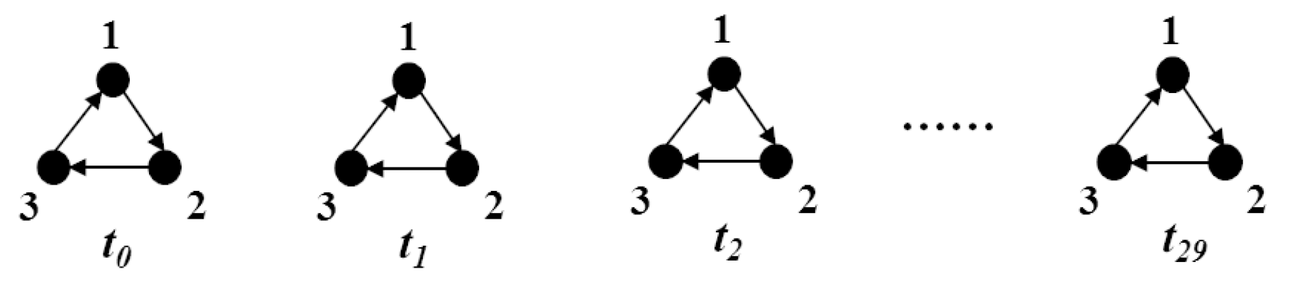
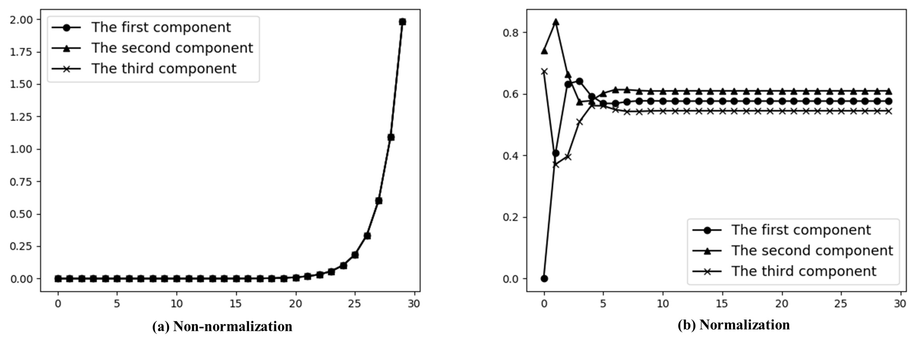
First, we explain the necessity of normalization by a simple example. Assuming that three nodes send messages regularly, we first generate a simple data streams including three nodes to illustrate normalization mentioned in Section 2.2, as shown in Figure 4.

Figure 5 is the label value of node 3 from $t_0$ to $t_{29}$ in the case of normalization and non-normalization, respectively. It is more realistic that the label values should remain stable over a certain period as the community evolution. For real data sets, the interactions between nodes are more complex. Figure 5b illustrates that normalization can ensure the label values of the nodes keep stable.

3.2. Community Detection and Tracking

This section we evaluate our method by real data sets. Firstly, different clustering methods are tested on $Students$, and then the results of TLW and other static community detection algorithms are given. Finally, we visualize our division result of $Students$ and $Facebook$.

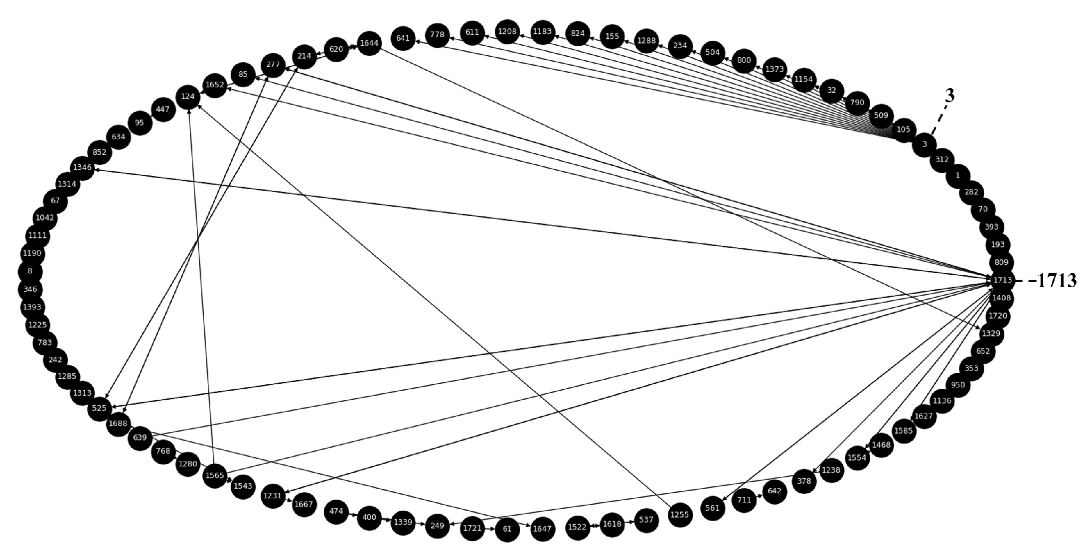
To evaluate results of different clustering methods based on (6), we use Students data set from 16:06:47 on 27 June 2014 to 23:58:51 on 27 June 2014 with 113 edges and 87 nodes. Figure 2 is the snapshot of the associated temporal network by mixing all edges together. Some obvious clusters can be observed around nodes 3 and 1713. Let the $c=1\times {10}^{-6}$ and $\beta =1,\alpha =1$. Compute label values of nodes at 23:58:51, and use clustering analysis methods to reveal nodes in same community. Since the number of communities is unknown, we group the nodes by AP and DBSCAN, respectively. According to the results of AP and DBSCAN, setting the number of clusters to be 21, we also use Mini Batch K-means to cluster. Focusing on two key nodes 3 and 1713, Figure 6 shows the results of community detection. According to the division of $X_u\left(t\right)$, community structure is in accordance with the actual situation and dependence on clustering algorithms is not strong. The modularity and running time of three methods are listed in

Table 1. Running time of different clustering methods.

Method	Mini Batch K-Means	DBSCAN	AP
1 day Modularity	0.773	0.684	0.674
1 day Running time(s)	$0.049\pm 0.005$	$0.003\pm 0.001$	$0.330\pm 0.008$
1 week Running time(s)	$0.106\pm 0.008$	$0.095\pm 0.003$	$2.523\pm 0.013$
2 months Running time(s)	$0.193\pm 0.011$	$0.786\pm 0.002$	$13.592\pm 0.046$

.

It is shown that modularity greater than about 0.3 appear to indicate significant community structure in practice [24], and typically fall in the range from 0.3 to 0.7 [1]. According to Table 1, we find that all three methods can get a good community structure with reasonable modularity, but AP is obviously more computational expensive than Mini Batch K-means and DBSCAN, which may make AP impractical in processing large-scale networks. Compared with other two methods, Mini Batch K-means gets better community structure and runs faster with the increase of data. If the community structure is stable in a certain period, DBSCAN method can be used firstly and then Mini Batch K-means can be used to approximate it. Mini Bath K-means is used in subsequent experiments. We choose node 525 (see Figure 6) to track the community evolution based on label value, the result is shown in Figure 7. Node 525 joins the community halfway, and does not interact directly with 1713.

The number of communities in this experiment is set to 21 for a network with 87 nodes. It may be too many for a real social network. One reason is that some nodes communicate little with other nodes, which makes them become noise points in clustering analysis. In the case of large-scale data sets, noise points are often categorized separately because of inadequate information of time.

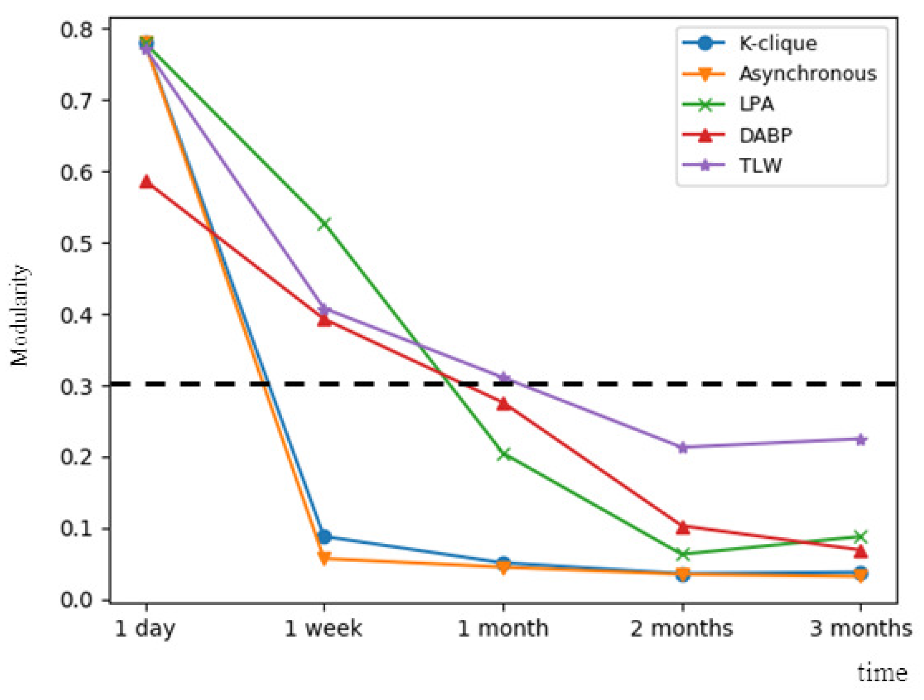
To evaluate our method in community detection, we compare modularity with other static community detection algorithms. We choose partial community detection methods that focus on static graph: K-clique [25], asynchronous label propagation [26] and label propagation [3]. The dynamic community detection algorithm of [6] called DABP is also included. Data streams on 27 June are mixed to an undirected snapshot with 87 nodes and 85 edges. The result is shown in

Table 2. The modularity of community structure from different methods tested on $Students$ with the increase of $\Delta t$.

Method	K-Clique	Asynchronous	Label Propagation	DABP	TLW
1 day	0.780	0.780	0.780	0.587	0.773
1 week	0.088	0.057	0.528	0.393	0.408
1 month	0.051	0.045	0.205	0.276	0.311
2 months	0.036	0.035	0.063	0.103	0.213
3 months	0.038	0.032	0.088	0.069	0.225

. All methods have a good performance with high modularity on the first day. Please note that our method is to reveal the community structure at 23:58:51. With the passing of time, Figure 8 shows the change of modularity of all methods. Here modularity of all methods decreases with the increase of time. Modularity of static methods decreases rapidly, while the modularity corresponding to TLW decreases much more slowly, which means that TLW has distinct advantages over other methods in maintaining a significant community structure. Although nodes in many networks fall naturally into communities, the time factor is very important. The community structure of the network is unstable. If only the snapshots are used to divide networks by mixing data streams, some disappeared or changed community structures are retained in snapshots which make community structure of snapshots vague. At this point, it is difficult for static algorithms to get a high modularity.

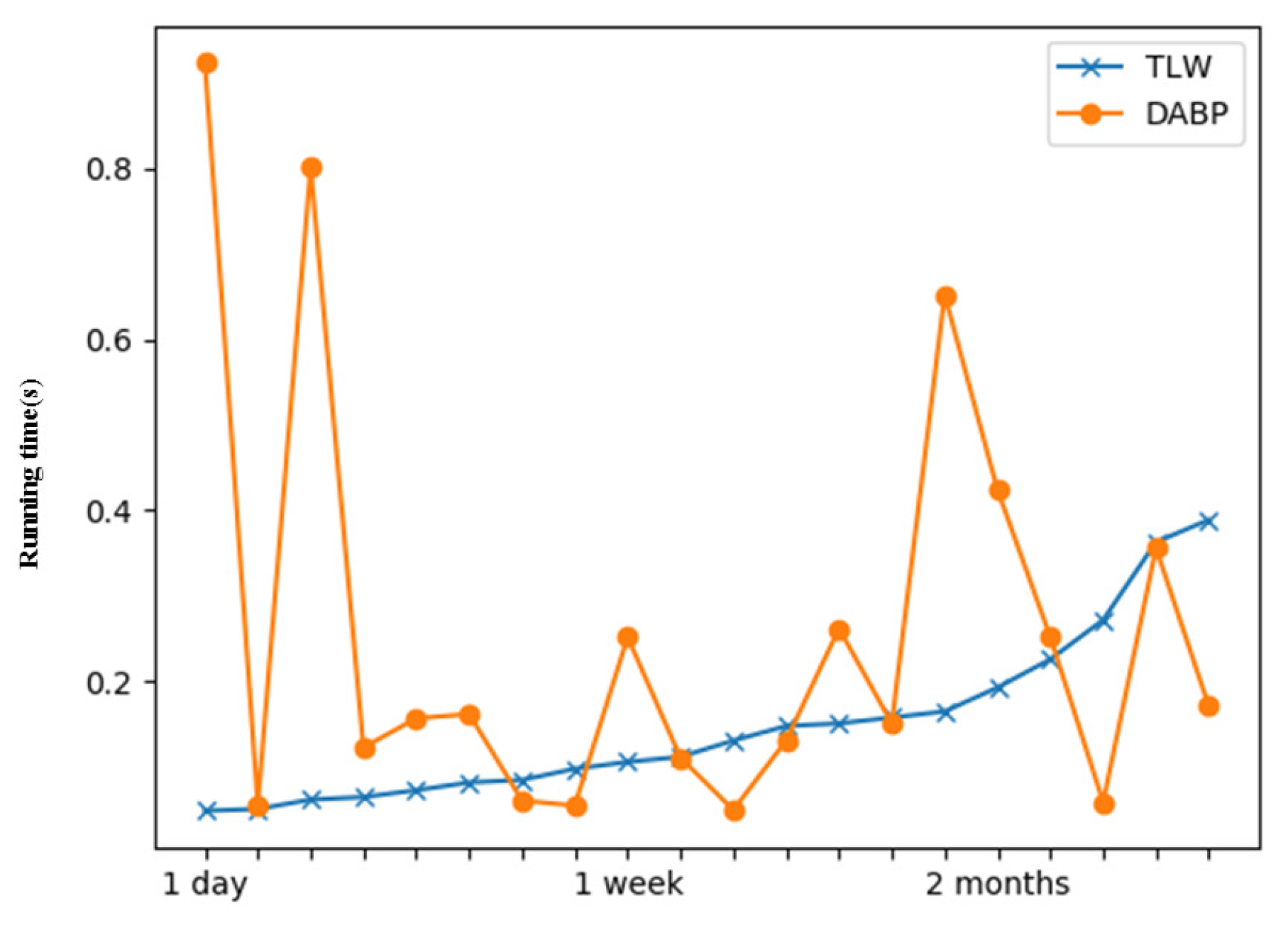
We also compute the running time of TLW and several related static methods. The results are listed in

Table 3. The running time with the increase of $\Delta t$ about different methods.

Method	K-Clique	Asynchronous	Label Propagation	TLW
1 day (s)	$0.021\pm 0.001$	$0.030\pm 0.021$	$0.024\pm 0.002$	$0.049\pm 0.005$
1 week (s)	$0.036\pm 0.008$	$0.077\pm 0.017$	$0.041\pm 0.012$	$0.106\pm 0.008$
1 month (s)	$0.098\pm 0.006$	$0.108\pm 0.009$	$0.097\pm 0.007$	$0.121\pm 0.007$
2 months (s)	$0.127\pm 0.312$	$0.156\pm 0.013$	$0.134\pm 0.011$	$0.193\pm 0.011$
3 months(s)	$0.264\pm 0.008$	$0.284\pm 0.075$	$0.340\pm 0.132$	$0.421\pm 0.013$
4 months (s)	$0.455\pm 0.059$	$0.665\pm 0.072$	$0.551\pm 0.072$	$0.879\pm 0.022$

. TLW can get the division of community structure almost as fast as classical static algorithms. Considering that DABP is an incremental algorithm, we compare the real-time running time of TLW and DABP separately. Choose 20 subgraphs from $G_0,G_1,\cdots ,G_n$ randomly and compute the time of processing each subgraph $G_i$, the result is shown in Figure 9. The real-time running time of TLW grows slowly and the running time of DABP depends on the scale of each subgraph. Our methods can get a higher modularity than DABP without consuming too much time.

We also visualize the community structure of $Students$ and $Facebook$ in three periods in Figure 10. Several communities with the high number of nodes are shown. More and more nodes become the members of community as time goes on, while accords with the facts in most social networks.

4. The Effects of Parameters

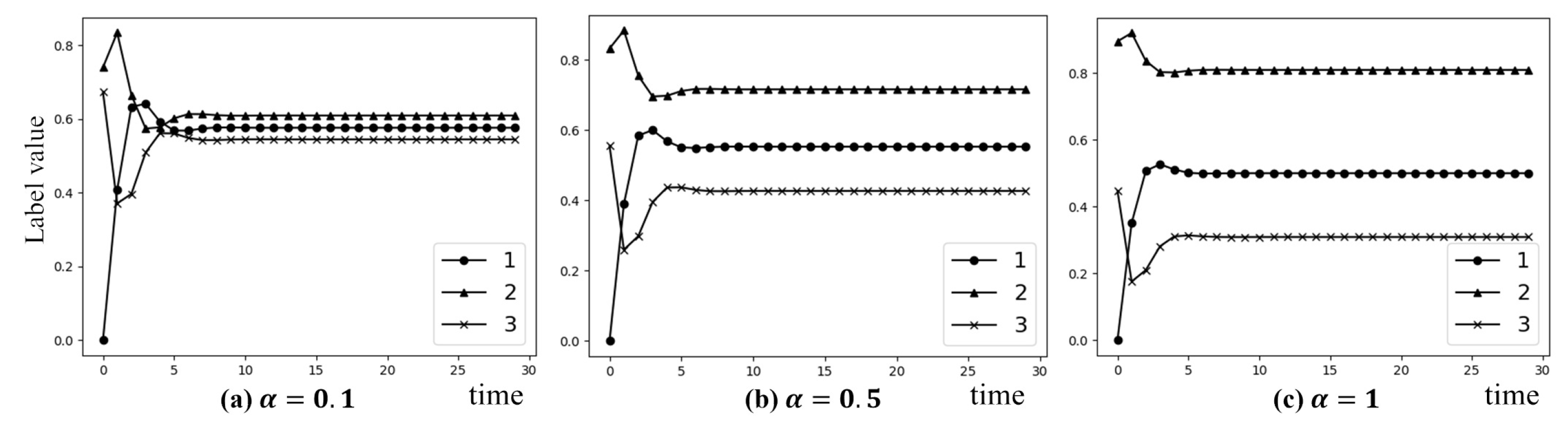
Three parameters, $c,\beta$ and $\alpha$ should be set manually in TLW, where $\alpha$ uses to control information intensity. A larger $\alpha$ means that information received recently is more important. Using artificial data set generated in Section 3.1, label value corresponding to different $\alpha$ is shown in Figure 11.

$\beta$ and c are time decay parameters which control the speed of exponential decay of information. c depends on time interval $\tau$ of data streams. We generate a new data streams to illustrate the effect of different $\beta$ and c. Similar to the artificial data streams generated in Section 3.1, at each $t_i$, now only one message passes in turn, we show this data streams in Figure 12.

Let $\alpha =0.1$. Fix $\beta$ and c respectively, the first component of $X_3\left(t\right)$ for different c and $\beta$ is given in Figure 13a,b. Variation of label value from peak to trough is not violently with $\beta =1,c=0.25$ or $\beta =1,c=0.1$, here $\tau =t_{i+1}-t_i$ is 1 s. c is more important than $\beta$ because $\tau$ range from 1 s to 1000 s or more in real data sets, it is suitable to consider c and $\tau$ together so that $e^{c\tau }$ can be a number between 0 and 1.

To make a further analysis of influence of different parameters on community detection, we choose $Students$ data set of the first day and fixing $\beta =1$. Using Mini Batch K-means methods and setting the number of clusters $n=14$, we show the effect of different c and $\alpha$ on modularity with Mini Bath K-means in

Table 4. The change of modularity with the increase of $\Delta t$ about different methods.

	$\mathit{\alpha }=0.2$	$\mathit{\alpha }=0.4$	$\mathit{\alpha }=0.6$	$\mathit{\alpha }=0.8$	$\mathit{\alpha }=1$
$c=1\times {10}^{-5}$	0.643	0.642	0.660	0.650	0.685
$c=2\times {10}^{-5}$	0.620	0.637	0.622	0.619	0.623
$c=4\times {10}^{-5}$	0.569	0.560	0.553	0.544	0.508
$c=6\times {10}^{-5}$	0.510	0.521	0.513	0.503	0.499
$c=8\times {10}^{-5}$	0.406	0.478	0.365	0.301	0.216
$c=1\times {10}^{-4}$	0.388	0.343	0.280	0.277	0.210

. Please note that modularity does not change linearly with c and $\alpha$, but depend on the data sets.

5. Conclusions

In this paper, we propose a community detection method TLW in temporal networks based on the label value $X_u\left(t\right)$ of each node u. TLW transfers community detection problem to clustering analysis in high-dimensional vector space. We validate the effectiveness of our algorithm. TLW can ensure that modularity of community divisions remains relatively reasonable high with the passing of time. We also show that it is hard for static community detection algorithms to divide community structure well in real data sets if only mix temporal data streams to snapshots. As an important part of community detection, only several simple clustering algorithms are discussed in this paper. Meanwhile, many dynamic community analysis algorithms have been integrated into a package [27] and it is convenient for user to compare their methods with classical dynamic community detection approaches. TLW is quite different from these methods and division of community is influenced by different evaluation criteria and data sets. A comprehensive comparison will be given in the future work.

References

- Newman, M.E.J. Finding and Evaluating Community Structure in Networks. Phys. Rev. E 2004, 69, 026113. [Google Scholar] [CrossRef] [PubMed]
- Kernighan, B.W.; Lin, S. An Efficient Heuristic Procedure for Partitioning Graphs. Bell Syst. Tech. J. 1970, 49, 291–307. [Google Scholar] [CrossRef]
- Cordasco, G.; Gargano, L. Community detection via semi-synchronous label propagation algorithms. In Proceedings of the 2010 IEEE International Workshop on Business Applications of Social Network Analysis (BASNA), Bangalore, India, 15 December 2010; pp. 1–8. [Google Scholar]
- Rosval, M.; Bergstrom, C.T. Mapping change in large networks. PLoS ONE 2010, 5, e8694. [Google Scholar] [CrossRef] [PubMed]
- Studholme, C.; Hill, D.L.G.; Hawkes, D.J. An overlap invariant entropy measure of 3D medical image alignment. Pattern Recognit. 1999, 32, 71–86. [Google Scholar] [CrossRef]
- Li, X.; Wu, B.; Guo, Q.; Zeng, X.; Shi, C. Dynamic community detection algorithm based on incremental identification. In Proceedings of the 2015 IEEE International Conference on Data Mining Workshop (ICDMW), Atlantic City, NJ, USA, 14–17 November 2015; pp. 900–907. [Google Scholar]
- Agarwal, P.; Verma, R.; Agarwal, A.; Chakraborty, T. DyPerm: Maximizing Permanence for Dynamic Community Detection. In Proceedings of the Pacific-Asia Conference on Knowledge Discovery and Data Mining, Melbourne, VIC, Australia, 3–6 June 2018; pp. 437–449. [Google Scholar]
- Guo, Q.; Zhang, L.; Wu, B.; Zeng, X. Dynamic community detection based on distance dynamics. In Proceedings of the 2016 IEEE/ACM International Conference on Advances in Social Networks Analysis and Mining (ASONAM), San Francisco, CA, USA, 18–21 August 2016; pp. 329–336. [Google Scholar]
- DiTursi, D.J.; Ghosh, G.; Bogdanov, P. Local community detection in dynamic networks. In Proceedings of the 2017 IEEE International Conference on Data Mining (ICDM), New Orleans, LA, USA, 18–21 November 2017; pp. 847–852. [Google Scholar]
- Xie, J.; Chen, M.; Szymanski, B.K. LabelrankT: Incremental community detection in dynamic networks via label propagation. In Proceedings of the Proceedings of the Workshop on Dynamic Networks Management and Mining, New York, NY, USA, 22–27 June 2013; pp. 25–32. [Google Scholar]
- Sattari, M.; Zamanifar, K. A cascade information diffusion based label propagation algorithm for community detection in dynamic social networks. J. Comput. Sci. 2018, 25, 122–133. [Google Scholar] [CrossRef]
- Panzarasa, P.; Opsahl, T.; Carley, K.M. Patterns and dynamics of users’ behavior and interaction: Network analysis of an online community. J. Am. Soc. Inf. Sci. Technol. 2009, 60, 911–932. [Google Scholar] [CrossRef]
- Rozenshtein, P.; Gionis, A. Temporal pagerank. In Proceedings of the Joint European Conference on Machine Learning and Knowledge Discovery in Databases, Riva del Garda, Italy, 19–23 September 2016; pp. 674–689. [Google Scholar]
- Béres, F.; Pálovics, R.; Oláh, A.; Benczúr, A.A. Temporal walk based centrality metric for graph streams. Appl. Netw. Sci. 2018, 3, 32. [Google Scholar] [CrossRef] [PubMed]
- Pons, P.; Latapy, M. Computing communities in large networks using random walks. J. Graph Algorithms Appl. 2006, 10, 191–218. [Google Scholar] [CrossRef]
- Cai, B.; Wang, H.; Zeng, H.; Wang, H. Evaluation repeated random walks in community detection of social networks. In Proceedings of the 2010 International Conference on Machine Learning and Cybernetics, Qingdao, China, 11–14 July 2010; pp. 1849–1854. [Google Scholar]
- De Meo, P.; Ferrara, E.; Fiumara, G.; Provetti, A. Enhancing community detection using a network weighting strategy. Inf. Sci. 2013, 222, 648–668. [Google Scholar] [CrossRef] [Green Version]
- De Meo, P.; Ferrara, E.; Fiumara, G.; Provetti, A. Mixing local and global information for community detection in large networks. J. Comput. Syst. Sci. 2014, 80, 72–87. [Google Scholar] [CrossRef]
- Rémy, C.; Rym, B.; Matthieu, L. Tracking bitcoin users activity using community detection on a network of weak signals. In Proceedings of the International Conference on Complex Networks and Their Applications, Lyon, France, 29 November–1 December 2017; pp. 166–177. [Google Scholar]
- Frey, B.J.; Dueck, D. Clustering by passing messages between data points. Science 2007, 315, 972–976. [Google Scholar] [CrossRef] [PubMed]
- Ester, M.; Kriegel, H.-P.; Sander, J.; Xu, X. A density-based algorithm for discovering clusters in large spatial databases with noise. In Proceedings of the Second International Conference on Knowledge Discovery and Data Mining, Portland, OQ, USA, 2–4 August 1996; pp. 226–231. [Google Scholar]
- Sculley, D. Web-scale k-means clustering. In Proceedings of the 19th International Conference on World Wide Web, Raleigh, NC, USA, 26–30 April 2010; pp. 1177–1178. [Google Scholar]
- Viswanath, B.; Mislove, A.; Cha, M.; Gummadi, K.P. On the evolution of user interaction in facebook. In Proceedings of the 2nd ACM Workshop on Online Social Networks, Barcelona, Spain, 17 August 2009; pp. 37–42. [Google Scholar]
- Newman, M.E. Fast algorithm for detecting community structure in networks. Phys. Rev. E 2004, 69, 066133. [Google Scholar] [CrossRef] [PubMed] [Green Version]
- Palla, G.; Derényi, I.; Farkas, I.; Vicsek, T. Uncovering the overlapping community structure of complex networks in nature and society. Nature 2005, 435, 814. [Google Scholar] [CrossRef] [PubMed]
- Raghavan, U.N.; Albert, R.; Kumara, S. Near linear time algorithm to detect community structures in large-scale networks. Phys. Rev. E 2007, 76, 036106. [Google Scholar] [CrossRef] [PubMed] [Green Version]
- Sarmento, R.P.; Lemos, L.; Cordeiro, M.; Rossetti, G.; Cardoso, D. DynComm R Package–Dynamic Community Detection for Evolving Networks. arXiv 2019, arXiv:1905.01498. [Google Scholar]
Figure 1.
Several different forms of data. (a) is the data used in structure-based methods, temporal data in a time window of size is mixed to snapshot . Incremental analysis in (b) knows the structure of network at the beginning and addition of nodes and edges (or delete) to change local structure so that the new communities grow. (c) is a real data set called where it is hard finding community structure at any and the information flow is spare when edges appear.
Figure 2.
Mixing all 113 edges appear on 87 nodes on 27 June 2014. It is easy to find that nodes 1713 and 3 interact more frequently with other nodes.
Figure 3.
Two different situations in temporal networks. (a) shows that two communities A and B share the same information exchange within community, the corresponding nodes are of the same importance but belong to different communities. (b) shows that nodes u and v are in different communities in the beginning and v sends a message to u at time . If v sends a message to u again at , as shown in (c), u will have a higher probability of belonging to B at than those nodes inside A send a message to u at , which is illustrated in (d).
Figure 4.
Three nodes send messages to each other in 30 s. The order that three nodes periodically send information at each time is , , .
Figure 5.
Label value of node 3 with non-normalization and normalization. The value increases exponentially without normalization (see (a)), but tends to be stable after normalization (see (b)).
Figure 6.
Results of community detection with AP, Mini Batch K-means, and DBSCAN. The blue nodes and node 3 are in the same community. The orange nodes belong to community of node 1713. The division is only different in a few points.
Figure 7.
Label value of node 525 from 16:06:47 to 23:58:51. The horizontal axis denotes the sequence of the interactions. This sequence starts from 0 and end at 97, indicating that there are 97 information interactions between nodes in this day.
Figure 8.
Modularity of different methods from one day to three months.
Figure 9.
Real-time running time of TLW and DABP.
Figure 10.
Community structure of and in one day, one week, and one month, respectively. Nodes in black denote that they do not belong to any community obviously yet.
Figure 11.
The effect of on the label value of node 3. The larger makes node 2 have more influence on node 3 than the others.
Figure 12.
Three nodes send messages in turn. The order is , , , .
Figure 13.
Fix and c respectively, and calculate the first component of . Two parameters are set to 0.25, 0.5, 0.75 and 1. Smaller c and larger both have smaller peak value and larger valley value.