Supervised Machine Learning Techniques to the Prediction of Tunnel Boring Machine Penetration Rate

 ,
,  ,
,  and
and
Abstract
:1. Introduction
2. Background of Supervised ML Models
2.1. K-Nearest Neighbor (KNN)
2.2. Support Vector Machine (SVM)
2.3. Neural Network (NN)
2.4. Classification and Regression Trees (CART)
2.5. Chi-Squared Automatic Interaction Detection (CHAID)
3. Materials and Methods
3.1. Model’s Assessment
3.2. Case Study and Data Preparation
4. Results and Discussion
4.1. Assessment of Models
4.2. Result of Selected Models
5. Conclusions
Author Contributions
Funding
Conflicts of Interest
Abbreviations
| ANNs | Artificial neural networks |
| AR | Advance rate |
| DPW | The distance between planes of weakness |
| α | The angle between plane of weakness and TBM-driven direction |
| RMR | Rock mass rating |
| GEP | Gene expression programing |
| CFF | Core fracture frequency |
| RPM | Revolution per minutes |
| UI | Utilization index |
| PSI | Peak slope index |
| Qu | Quartz percentage |
| Rs | Rotational speed of TBM |
| Js | Joint spacing |
| Jc | Joint condition |
| C | Cohesion |
| φ | Friction angle |
| υ | Poisson’s ratio |
| SE | Specific energy |
| TF | Thrust force |
| CT | Cutterhead power |
| ELM | Extreme learning machine |
| N | Overload factor |
| WTS | Water table surface |
| DE | Differential evolution |
| BNNs | Biological neural networks |
| HS-BFGS | Hybrid harmony search |
| ICA | Imperialism competitive algorithm |
| GWO | Grey wolf optimizer |
| BPNNs | Back-propagation neural networks |
| ANFIS | Adoptive neuro-fuzzy inference system |
| CART | classification and regression trees |
| CHAID | chi-squared automatic interaction detection |
| CSM | Colorado school of mines |
| DNNs | Deep neural networks |
| FIS | Fuzzy inference system |
| FA | Firefly algorithm |
| KNN | k-nearest neighbor |
| logsig | Log-sigmoid transfer function |
| ML | machine learning |
| PR | penetration rate |
| PSO | particle swarm optimization |
| purelin | Linear transfer function |
| SVM | support vector machine |
| tansig | Hyperbolic tangent Sigmoid transfer function |
| TBM | Tunnel boring machine |
| UCS | uniaxial compressive strength |
References
- Roxborough, F.F.; Phillips, H.R. Rock excavation by disc cutter. Int. J. Rock Mech. Min. Sci. Geomech. Abstr. 1975, 12, 361–366. [Google Scholar] [CrossRef]
- Snowdon, R.; Ryley, M.; Temporal, J. A study of disc cutting in selected British rocks. Int. J. Rock Mech. Min. Sci. Geomech. Abstr. 1982, 19, 107–121. [Google Scholar] [CrossRef]
- Sanio, H. Prediction of the performance of disc cutters in anisotropic rock. Int. J. Rock Mech. Min. Sci. Geomech. Abstr. 1985, 22, 153–161. [Google Scholar] [CrossRef]
- Sato, K.; Gong, F.; Itakura, K. Prediction of disc cutter performance using a circular rock cutting ring. In Proceedings of the 1st International Mine Mechanization and Automation Symposium, Golden, CO, USA, 10–13 June 1991. [Google Scholar]
- Rostami, J. Development of a force Estimation Model for Rock Fragmentation with Disc Cutters through Theoretical Modeling and Physical Measurement of Crushed Zone Pressure. Ph.D. Thesis, Colorado School of Mines, Golden, CO, USA, 1997. [Google Scholar]
- Yagiz, S. Utilizing rock mass properties for predicting TBM performance in hard rock condition. Tunn. Undergr. Space Technol. 2008, 23, 326–339. [Google Scholar] [CrossRef]
- Gong, Q.-M.; Zhao, J. Development of a rock mass characteristics model for TBM penetration rate prediction. Int. J. Rock Mech. Min. Sci. 2009, 46, 8–18. [Google Scholar] [CrossRef]
- Farmer, I.W.; Glossop, N.H. Mechanics of disc cutter penetration. Tunn. Tunn. 1980, 12, 22–25. [Google Scholar]
- Ozdemir, L. Development of Theoretical Equations for Predicting Tunnel Boreability. Ph.D. Thesis, Colorado School of Mines, Golden, CO, USA, 1977. [Google Scholar]
- Yagiz, S.; Ozdemir, L. Geotechnical parameters influencing the TBM performance in various rocks. In Proceedings of the Program with Abstract, 44th Annual Meeting of Association of Engineering Geologists, Saint Louis, MO, USA, 12–14 June 2001; p. 79. [Google Scholar]
- Yagiz, S. Development of Rock Fracture and Brittleness Indices to Quantify the Effects of Rock Mass Features and Toughness in the CSM Model Basic Penetration for Hard Rock Tunneling Machines. Ph.D. Thesis, Colorado School of Mines, Golden, CO, USA, 2002. [Google Scholar]
- Armaghani, D.J.; Mohamad, E.T.; Narayanasamy, M.S.; Narita, N.; Yagiz, S. Development of hybrid intelligent models for predicting TBM penetration rate in hard rock condition. Tunn. Undergr. Space Technol. 2017, 63, 29–43. [Google Scholar] [CrossRef]
- Koopialipoor, M.; Nikouei, S.S.; Marto, A.; Fahimifar, A.; Armaghani, D.J.; Mohamad, E.T. Predicting tunnel boring machine performance through a new model based on the group method of data handling. Bull. Eng. Geol. Environ. 2018, 78, 3799–3813. [Google Scholar] [CrossRef]
- Yang, H.; Liu, J.; Liu, B. Investigation on the cracking character of jointed rock mass beneath TBM disc cutter. Rock Mech. Rock Eng. 2018, 51, 1263–1277. [Google Scholar] [CrossRef]
- Yang, H.; Wang, H.; Zhou, X. Analysis on the damage behavior of mixed ground during TBM cutting process. Tunn. Undergr. Space Technol. 2016, 57, 55–65. [Google Scholar] [CrossRef]
- Yang, H.Q.; Zeng, Y.Y.; Lan, Y.F.; Zhou, X.P. Analysis of the excavation damaged zone around a tunnel accounting for geostress and unloading. Int. J. Rock Mech. Min. Sci. 2014, 69, 59–66. [Google Scholar] [CrossRef]
- Yagiz, S.; Gokceoglu, C.; Sezer, E.; Iplikci, S. Application of two non-linear prediction tools to the estimation of tunnel boring machine performance. Eng. Appl. Artif. Intell. 2009, 22, 808–814. [Google Scholar] [CrossRef]
- Hamidi, J.K.; Shahriar, K.; Rezai, B.; Bejari, H. Application of fuzzy set theory to rock engineering classification systems: An illustration of the rock mass excavability index. Rock Mech. Rock Eng. 2010, 43, 335–350. [Google Scholar] [CrossRef]
- Grima, M.A.; Bruines, P.A.; Verhoef, P.N.W. Modeling tunnel boring machine performance by neuro-fuzzy methods. Tunn. Undergr. Space Technol. 2000, 15, 259–269. [Google Scholar] [CrossRef]
- Farrokh, E.; Rostami, J.; Laughton, C. Study of various models for estimation of penetration rate of hard rock TBMs. Tunn. Undergr. Space Technol. 2012, 30, 110–123. [Google Scholar] [CrossRef]
- Chen, H.; Asteris, P.G.; Jahed Armaghani, D.; Gordan, B.; Pham, B.T. Assessing Dynamic Conditions of the Retaining Wall: Developing Two Hybrid Intelligent Models. Appl. Sci. 2019, 9, 1042. [Google Scholar] [CrossRef]
- Asteris, P.G.; Nikoo, M. Artificial bee colony-based neural network for the prediction of the fundamental period of infilled frame structures. Neural Comput. Appl. 2019. [Google Scholar] [CrossRef]
- Moayedi, H.; Armaghani, D.J. Optimizing an ANN model with ICA for estimating bearing capacity of driven pile in cohesionless soil. Eng. Comput. 2018, 34, 347–356. [Google Scholar] [CrossRef]
- Yang, H.; Hasanipanah, M.; Tahir, M.M.; Bui, D.T. Intelligent Prediction of Blasting-Induced Ground Vibration Using ANFIS Optimized by GA and PSO. Nat. Resour. Res. 2019. [Google Scholar] [CrossRef]
- Armaghani, D.J.; Hajihassani, M.; Mohamad, E.T.; Marto, A.; Noorani, S.A. Blasting-induced flyrock and ground vibration prediction through an expert artificial neural network based on particle swarm optimization. Arab. J. Geosci. 2014, 7, 5383–5396. [Google Scholar] [CrossRef]
- Asteris, P.G.; Nozhati, S.; Nikoo, M.; Cavaleri, L.; Nikoo, M. Krill herd algorithm-based neural network in structural seismic reliability evaluation. Mech. Adv. Mater. Struct. 2018, 26, 1146–1153. [Google Scholar] [CrossRef]
- Asteris, P.G.; Plevris, V. Anisotropic masonry failure criterion using artificial neural networks. Neural Comput. Appl. 2017, 28, 2207–2229. [Google Scholar] [CrossRef]
- Faradonbeh, R.S.; Armaghani, D.J.; Amnieh, H.B.; Mohamad, E.T. Prediction and minimization of blast-induced flyrock using gene expression programming and firefly algorithm. Neural Comput. Appl. 2016, 29, 269–281. [Google Scholar] [CrossRef]
- Sarir, P.; Chen, J.; Asteris, P.G.; Armaghani, D.J.; Tahir, M.M. Developing GEP tree-based, neuro-swarm, and whale optimization models for evaluation of bearing capacity of concrete-filled steel tube columns. Eng. Comput. 2019. [Google Scholar] [CrossRef]
- Cavaleri, L.; Chatzarakis, G.E.; Trapani, F.D.; Douvika, M.G.; Roinos, K.; Vaxevanidis, N.M.; Asteris, P.G. Modeling of surface roughness in electro-discharge machining using artificial neural networks. Adv. Mater. Res. 2017, 6, 169–184. [Google Scholar]
- Zhou, J.; Li, E.; Yang, S.; Wang, M.; Shi, X.; Yao, S.; Mitri, H.S. Slope stability prediction for circular mode failure using gradient boosting machine approach based on an updated database of case histories. Saf. Sci. 2019, 118, 505–518. [Google Scholar] [CrossRef]
- Guo, H.; Zhou, J.; Koopialipoor, M.; Armaghani, D.J.; Tahir, M.M. Deep neural network and whale optimization algorithm to assess flyrock induced by blasting. Eng. Comput. 2019. [Google Scholar] [CrossRef]
- Mahdiyar, A.; Armaghani, D.J.; Marto, A.; Nilashi, M.; Ismail, S. Rock tensile strength prediction using empirical and soft computing approaches. Bull. Eng. Geol. Environ. 2019, 78, 4519–4531. [Google Scholar] [CrossRef]
- Zhou, J.; Li, X.; Mitri, H.S. Classification of rockburst in underground projects: comparison of ten supervised learning methods. J. Comput. Civ. Eng. 2016, 30, 04016003. [Google Scholar] [CrossRef]
- Zhou, J.; Li, X.; Mitri, H.S. Comparative performance of six supervised learning methods for the development of models of hard rock pillar stability prediction. Nat. Hazards 2015, 79, 291–316. [Google Scholar] [CrossRef]
- Benardos, A.G.; Kaliampakos, D.C. Modelling TBM performance with artificial neural networks. Tunn. Undergr. Space Technol. 2004, 19, 597–605. [Google Scholar] [CrossRef]
- Armaghani, D.J.; Koopialipoor, M.; Marto, A.; Yagiz, S. Application of several optimization techniques for estimating TBM advance rate in granitic rocks. J. Rock Mech. Geotech. Eng. 2019, 11, 779–789. [Google Scholar] [CrossRef]
- Armaghani, D.J.; Faradonbeh, R.S.; Momeni, E.; Fahimifar, A.; Tahir, M.M. Performance prediction of tunnel boring machine through developing a gene expression programming equation. Eng. Comput. 2018, 34, 129–141. [Google Scholar] [CrossRef]
- Eftekhari, M.; Baghbanan, A.; Bayati, M. Predicting penetration rate of a tunnel boring machine using artificial neural network. In Proceedings of the ISRM International Symposium-6th Asian Rock Mechanics Symposium; International Society for Rock Mechanics, New Delhi, India, 23–27 October 2010. [Google Scholar]
- Javad, G.; Narges, T. Application of artificial neural networks to the prediction of tunnel boring machine penetration rate. Min. Sci. Technol. 2010, 20, 727–733. [Google Scholar] [CrossRef]
- Gholami, M.; Shahriar, K.; Sharifzadeh, M.; Hamidi, J.K. A comparison of artificial neural network and multiple regression analysis in TBM performance prediction. In Proceedings of the ISRM Regional Symposium-7th Asian Rock Mechanics Symposium; International Society for Rock Mechanics, Seoul, Korea, 15–19 October 2012. [Google Scholar]
- Salimi, A.; Esmaeili, M. Utilising of linear and non-linear prediction tools for evaluation of penetration rate of tunnel boring machine in hard rock condition. Int. J. Min. Miner. Eng. 2013, 4, 249–264. [Google Scholar] [CrossRef]
- Torabi, S.R.; Shirazi, H.; Hajali, H.; Monjezi, M. Study of the influence of geotechnical parameters on the TBM performance in Tehran–Shomal highway project using ANN and SPSS. Arab. J. Geosci. 2013, 6, 1215–1227. [Google Scholar] [CrossRef]
- Shao, C.; Li, X.; Su, H. Performance Prediction of Hard Rock TBM Based on Extreme Learning Machine. In Proceedings of the International Conference on Intelligent Robotics and Applications, Busan, Korea, 25–28 September 2013; pp. 409–416. [Google Scholar]
- Mahdevari, S.; Shahriar, K.; Yagiz, S.; Shirazi, M.A. A support vector regression model for predicting tunnel boring machine penetration rates. Int. J. Rock Mech. Min. Sci. 2014, 72, 214–229. [Google Scholar] [CrossRef]
- Koopialipoor, M.; Fahimifar, A.; Ghaleini, E.N.; Momenzadeh, M.; Armaghani, D.J. Development of a new hybrid ANN for solving a geotechnical problem related to tunnel boring machine performance. Eng. Comput. 2019. [Google Scholar] [CrossRef]
- Koopialipoor, M.; Tootoonchi, H.; Jahed Armaghani, D.; Tonnizam Mohamad, E.; Hedayat, A. Application of deep neural networks in predicting the penetration rate of tunnel boring machines. Bull. Eng. Geol. Environ. 2019. [Google Scholar] [CrossRef]
- Hasanipanah, M.; Monjezi, M.; Shahnazar, A.; Armaghani, D.J.; Farazmand, A. Feasibility of indirect determination of blast induced ground vibration based on support vector machine. Measurement 2015, 75, 289–297. [Google Scholar] [CrossRef]
- Liang, M.; Mohamad, E.T.; Faradonbeh, R.S.; Jahed Armaghani, D.; Ghoraba, S. Rock strength assessment based on regression tree technique. Eng. Comput. 2016, 32, 343–354. [Google Scholar] [CrossRef]
- Khandelwal, M.; Armaghani, D.J.; Faradonbeh, R.S.; Yellishetty, M.; Majid, M.Z.A.; Monjezi, M. Classification and regression tree technique in estimating peak particle velocity caused by blasting. Eng. Comput. 2017, 33, 45–53. [Google Scholar] [CrossRef]
- Jamshidi, A. Prediction of TBM penetration rate from brittleness indexes using multiple regression analysis. Model. Earth Syst. Environ. 2018, 4, 383–394. [Google Scholar] [CrossRef] [Green Version]
- Shijing, W.; Bo, Q.; Zhibo, G. The time and cost prediction of tunnel boring machine in tunnelling. Wuhan Univ. J. Nat. Sci. 2006, 11, 385–388. [Google Scholar] [CrossRef]
- Sundaram, M. The effects of ground conditions on TBM performance in tunnel excavation—A case history. In Proceedings of the 10th Australia New Zealand conference on Geomechanics, Queensland, Australia, 21–24 October 2007. [Google Scholar]
- Ietto, F.; Perri, F.; Cella, F. Weathering characterization for landslides modeling in granitoid rock masses of the Capo Vaticano promontory (Calabria, Italy). Landslides 2018, 15, 43–62. [Google Scholar] [CrossRef]
- Ietto, F.; Perri, F.; Cella, F. Geotechnical and landslide aspects in weathered granitoid rock masses (Serre Massif, southern Calabria, Italy). Catena 2016, 145, 301–315. [Google Scholar] [CrossRef]
- Abad, S.V.A.N.K.; Tugrul, A.; Gokceoglu, C.; Armaghani, D.J. Characteristics of weathering zones of granitic rocks in Malaysia for geotechnical engineering design. Eng. Geol. 2016, 200, 94–103. [Google Scholar] [CrossRef]
- Yang, H.Q.; Li, Z.; Jie, T.Q.; Zhang, Z.Q. Effects of joints on the cutting behavior of disc cutter running on the jointed rock mass. Tunn. Undergr. Space Technol. 2018, 81, 112–120. [Google Scholar] [CrossRef]
- Duda, R.O.; Hart, P.E.; Stork, D.G. Pattern Classification and Scene Analysis; Wiley: New York, NY, USA, 1973; Volume 3. [Google Scholar]
- Franco-Lopez, H.; Ek, A.R.; Bauer, M.E. Estimation and mapping of forest stand density, volume, and cover type using the k-nearest neighbors method. Remote Sens. Environ. 2001, 77, 251–274. [Google Scholar] [CrossRef]
- Wu, X.; Kumar, V.; Quinlan, J.R.; Ghosh, J.; Yang, Q.; Motoda, H.; McLachlan, G.J.; Ng, A.; Liu, B.; Philip, S.Y. Top 10 algorithms in data mining. Knowl. Inf. Syst. 2008, 14, 1–37. [Google Scholar] [CrossRef]
- Akbulut, Y.; Sengur, A.; Guo, Y.; Smarandache, F. NS-k-NN: Neutrosophic set-based k-nearest neighbors classifier. Symmetry 2017, 9, 179. [Google Scholar] [CrossRef]
- Wei, C.; Huang, J.; Mansaray, L.; Li, Z.; Liu, W.; Han, J. Estimation and mapping of winter oilseed rape LAI from high spatial resolution satellite data based on a hybrid method. Remote Sens. 2017, 9, 488. [Google Scholar] [CrossRef]
- Qian, Y.; Zhou, W.; Yan, J.; Li, W.; Han, L. Comparing machine learning classifiers for object-based land cover classification using very high resolution imagery. Remote Sens. 2015, 7, 153–168. [Google Scholar] [CrossRef]
- Vapnik, V.; Vapnik, V. Statistical Learning Theory; Wiley: New York, NY, USA, 1998; pp. 156–160. [Google Scholar]
- Kavzoglu, T.; Sahin, E.K.; Colkesen, I. Landslide susceptibility mapping using GIS-based multi-criteria decision analysis, support vector machines, and logistic regression. Landslides 2014, 11, 425–439. [Google Scholar] [CrossRef]
- Cortes, C.; Vapnik, V. Support-vector networks. Mach. Learn. 1995, 20, 273–297. [Google Scholar] [CrossRef]
- Hong, H.; Pradhan, B.; Bui, D.T.; Xu, C.; Youssef, A.M.; Chen, W. Comparison of four kernel functions used in support vector machines for landslide susceptibility mapping: A case study at Suichuan area (China). Geomat. Nat. Hazards Risk 2017, 8, 544–569. [Google Scholar] [CrossRef]
- Kalantar, B.; Pradhan, B.; Naghibi, S.A.; Motevalli, A.; Mansor, S. Assessment of the effects of training data selection on the landslide susceptibility mapping: A comparison between support vector machine (SVM), logistic regression (LR) and artificial neural networks (ANN). Geomat. Nat. Hazards Risk 2018, 9, 49–69. [Google Scholar] [CrossRef]
- Hopfield, J.J. Neural networks and physical systems with emergent collective computational abilities. Proc. Natl. Acad. Sci. USA 1982, 79, 2554–2558. [Google Scholar] [CrossRef]
- Breiman, L.; Friedman, J.; Olshen, R.; Stone, C. Classification and Regression Trees; Taylor & Francis Group: New York, NY, USA, 1984; Volume 37, pp. 237–251. [Google Scholar]
- Kass, G.V. An exploratory technique for investigating large quantities of categorical data. J. R. Stat. Soc. Ser. C 1980, 29, 119–127. [Google Scholar] [CrossRef]
- Toghroli, A.; Suhatril, M.; Ibrahim, Z.; Safa, M.; Shariati, M.; Shamshirband, S. Potential of soft computing approach for evaluating the factors affecting the capacity of steel–concrete composite beam. J. Intell. Manuf. 2018, 29, 1793–1801. [Google Scholar] [CrossRef]
- Jian, Z.; Shi, X.; Huang, R.; Qiu, X.; Chong, C. Feasibility of stochastic gradient boosting approach for predicting rockburst damage in burst-prone mines. Trans. Nonferrous Met. Soc. China 2016, 26, 1938–1945. [Google Scholar]
- Zhou, J.; Li, E.; Wang, M.; Chen, X.; Shi, X.; Jiang, L. Feasibility of Stochastic Gradient Boosting Approach for Evaluating Seismic Liquefaction Potential Based on SPT and CPT Case Histories. J. Perform. Constr. Facil. 2019, 33, 4019024. [Google Scholar] [CrossRef]
- Zhou, J.; Shi, X.; Du, K.; Qiu, X.; Li, X.; Mitri, H.S. Feasibility of random-forest approach for prediction of ground settlements induced by the construction of a shield-driven tunnel. Int. J. Geomech. 2016, 17, 4016129. [Google Scholar] [CrossRef]
- Asteris, P.; Roussis, P.; Douvika, M. Feed-forward neural network prediction of the mechanical properties of sandcrete materials. Sensors 2017, 17, 1344. [Google Scholar] [CrossRef] [PubMed]
- Asteris, P.G.; Kolovos, K.G. Self-compacting concrete strength prediction using surrogate models. Neural Comput. Appl. 2019, 31, 409–424. [Google Scholar] [CrossRef]
- Liao, X.; Khandelwal, M.; Yang, H.; Koopialipoor, M.; Murlidhar, B.R. Effects of a proper feature selection on prediction and optimization of drilling rate using intelligent techniques. Eng. Comput. 2019. [Google Scholar] [CrossRef]
- Koopialipoor, M.; Jahed Armaghani, D.; Haghighi, M.; Ghaleini, E.N. A neuro-genetic predictive model to approximate overbreak induced by drilling and blasting operation in tunnels. Bull. Eng. Geol. Environ. 2019, 78, 981–990. [Google Scholar] [CrossRef]
- Swingler, K. Applying Neural Networks: A Practical Guide; Academic Press: New York, NY, USA, 1996; ISBN 0126791708. [Google Scholar]
- Looney, C.G. Advances in feedforward neural networks: Demystifying knowledge acquiring black boxes. IEEE Trans. Knowl. Data Eng. 1996, 8, 211–226. [Google Scholar] [CrossRef]
- Shams, S.; Monjezi, M.; Majd, V.J.; Armaghani, D.J. Application of fuzzy inference system for prediction of rock fragmentation induced by blasting. Arab. J. Geosci. 2015, 8, 10819–10832. [Google Scholar] [CrossRef]
- Zorlu, K.; Gokceoglu, C.; Ocakoglu, F.; Nefeslioglu, H.A.; Acikalin, S. Prediction of uniaxial compressive strength of sandstones using petrography-based models. Eng. Geol. 2008, 96, 141–158. [Google Scholar] [CrossRef]
- Bruines, P. Neuro-fuzzy modeling of TBM performance with emphasis on the penetration rate. Mem. Cent. Eng. Geol. Neth. Delft 1998, 173, 202. [Google Scholar]
- Sapigni, M.; Berti, M.; Bethaz, E.; Busillo, A.; Cardone, G. TBM performance estimation using rock mass classifications. Int. J. Rock Mech. Min. Sci. 2002, 39, 771–788. [Google Scholar] [CrossRef]
- Ulusay, R.; Hudson, J.A. ISRM (2007) The Complete ISRM Suggested Methods for Rock Characterization, Testing and Monitoring: 1974–2006; ISRM Turkish National Group: Ankara, Turkey, 2007; p. 628. [Google Scholar]
- Calcaterra, D.; Parise, M. Landslide types and their relationships with weathering in a Calabrian basin, southern Italy. Bull. Eng. Geol. Environ. 2005, 64, 193–207. [Google Scholar] [CrossRef]
- Jahed Armaghani, D.; Mohd Amin, M.F.; Yagiz, S.; Faradonbeh, R.S.; Abdullah, R.A. Prediction of the uniaxial compressive strength of sandstone using various modeling techniques. Int. J. Rock Mech. Min. Sci. 2016, 85, 174–186. [Google Scholar] [CrossRef]
- Bejarbaneh, B.Y.; Bejarbaneh, E.Y.; Fahimifar, A.; Armaghani, D.J.; Majid, M.Z.A. Intelligent modelling of sandstone deformation behaviour using fuzzy logic and neural network systems. Bull. Eng. Geol. Environ. 2018, 77, 345–361. [Google Scholar] [CrossRef]
- Yang, H.Q.; Lan, Y.F.; Lu, L.; Zhou, X.P. A quasi-three-dimensional spring-deformable-block model for runout analysis of rapid landslide motion. Eng. Geol. 2015, 185, 20–32. [Google Scholar] [CrossRef]
- Zhou, X.P.; Yang, H.Q. Micromechanical modeling of dynamic compressive responses of mesoscopic heterogenous brittle rock. Theor. Appl. Fract. Mech. 2007, 48, 1–20. [Google Scholar] [CrossRef]
- Yang, H.Q.; Xing, S.G.; Wang, Q.; Li, Z. Model test on the entrainment phenomenon and energy conversion mechanism of flow-like landslides. Eng. Geol. 2018, 239, 119–125. [Google Scholar] [CrossRef]
- Bieniawski, Z.T. Rock Mechanics Design in Mining and Tunnelling; A.A. Balkema: Rotterdam, The Netherlands, 1984; ISBN 9061915074. [Google Scholar]
- Innaurato, N.; Mancini, A.; Rondena, E.; Zaninetti, A. Forecasting and effective TBM performances in a rapid excavation of a tunnel in Italy. In Proceedings of the 7th ISRM Congress; International Society for Rock Mechanics and Rock Engineering, Aachen, Germany, 16–20 September 1991. [Google Scholar]
- Ribacchi, R.; Fazio, A.L. Influence of rock mass parameters on the performance of a TBM in a gneissic formation (Varzo Tunnel). Rock Mech. Rock Eng. 2005, 38, 105–127. [Google Scholar] [CrossRef]


| Reference | Technique | Parameters | Datasets/Description | |
|---|---|---|---|---|
| Input | Output | |||
| Alvarez Grima [19] | ANN | CFF, Dc, RPM, TF, UCS | AR, PR | 640 TBM projects |
| Bernardos and Kaliampakos [36] | ANN | N, overburden, permeability, RMR, rock mass weathering RQD, UCS, WTS, | AR | Athens metro tunnel |
| Yagiz [17] | ANN | BI, DPW, UCS, α | PR | 151 datasets |
| Eftekhari et al. [39] | ANN | BTS, CT, Qu, RMR, Rock Type, RQD, Rs TF, UCS | PR | 10 km data excavated in a tunnel |
| Gholamnejad and Tayarani [40] | ANN | DPW, RQD, UCS | PR | 185 datasets |
| Gholami et al. [41] | ANN | Jc, Js, RQD, UCS | PR | 121 tunnel sections |
| Salimi and Esmaeili [42] | ANN | BTS, DPW, PSI, UCS, α | PR | 46 sections of a water supply tunnel |
| Torabi et al. [43] | ANN | C, UCS, υ, φ | PR, UI | 39 sections of a highway project |
| Shao et al. [44] | ELM | BTS, DPW, PSI, UCS, α | PR | 153 datasets |
| Mahdevari et al. [45] | SVR | BI, BTS, CP, CT, DPW, SE, TF, UCS, α | PR | 150 datasets |
| Armaghani et al. [12] | PSO-ANN, ICA-ANN | BTS, UCS, RMR, RQD, TF, WZ, RPM | PR | 1286 datasets |
| Armaghani et al. [37] | PSO-ANN, ICA-ANN | Qu, BTS, UCS, RMR, RQD, TF, WZ, RPM | AR | 1286 datasets |
| Koopialipoor et al. [46] | FA-ANN | BTS, UCS, RMR, RQD, TF, WZ, RPM | PR | 1200 datasets |
| Koopialipoor et al. [47] | DNN | BTS, UCS, RMR, RQD, TF, WZ, RPM | PR | 1286 datasets |
| KNN | SVM |
| Number of nearest neighbors (k): Minimum 3 and maximum 5 Distance computation: Euclidean metric Prediction for range target: Mean of nearest neighbor values Stopping criteria: Stop when the 10 features have been selected | Stopping criteria: 1.E-3 Regularization parameter (C): 10 Regression precision (epsilon): 0.1 Kernel type: RBF RBF gamma: 0.1 |
| NN | CHAID |
| NN model: Multilayer perceptron (MLP) Stopping rules: Use maximum training time (per component model): 15 minutes Combining rule for continuous targets: Mean Number of component models for boosting and/or bagging: 10 Overfit prevention set (%): 30 Missing values in predictors: Delete listwise | Tree growing algorithm: CHAID Maximum tree depth: 5 Minimum records in parent branch (%): 2 Minimum records in child branch (%): 1 Combining rule for continuous targets: Mean Number of component models for boosting and/or bagging: 10 Significance level for splitting: 0.05 Significance level for merging: 0.05 Adjust significance values using Boferroni method Minimum change in expected cell frequencies: 0.001 Maximum iterations for convergence: 100 |
| CART | |
| Maximum tree depth: 5 Prune tree to avoid overfitting: maximum surrogates: 5 Minimum records in parent branch (%): 2 Minimum records in child branch (%): 1 Combining rule for continuous targets: mean Number of component models for boosting and/or bagging: 10 Minimum change in impurity: 0.0001 Over-fit prevention set (%): 30 | |
| Parameter | Type | Symbol | Unit | Min | Max | Average | St Dev |
|---|---|---|---|---|---|---|---|
| Rock quality designation | Input | RQD | % | 10 | 95 | 53.5 | 27.7 |
| Uniaxial compressive strength | UCS | MPa | 49 | 185 | 122.7 | 40.7 | |
| Weathering zone | WZ | - | 1 | 3 | 1.8 | 0.8 | |
| Brazilian tensile strength | BTS | MPa | 4.69 | 15.1 | 9.6 | 3.2 | |
| Thrust force per cutter | TF | kN | 83 | 513.5 | 276.8 | 133.1 | |
| Revolution per minute | RPM | rev/min | 4.5 | 11.9 | 8.6 | 2.4 | |
| Penetration rate | Output | PR | m/h | 1.11 | 3.75 | 2.4 | 0.6 |
| Method | Stage | R2 | RMSE | VAF | MAE | a20-Index | R2 Rank | RMSE Rank | VAF Rank | MAE Rank | a20-Index Rank | Total Rate |
|---|---|---|---|---|---|---|---|---|---|---|---|---|
| NN | TS | 0.924 | 0.180 | 91.735 | 0.137 | 0.944 | 5 | 5 | 5 | 5 | 4 | 24 |
| TR | 0.916 | 0.173 | 91.602 | 0.136 | 0.967 | 1 | 2 | 1 | 1 | 2 | 7 | |
| SVM | TS | 0.914 | 0.183 | 91.393 | 0.139 | 0.981 | 4 | 4 | 4 | 4 | 5 | 21 |
| TR | 0.942 | 0.144 | 94.207 | 0.114 | 0.987 | 3 | 4 | 3 | 2 | 4 | 16 | |
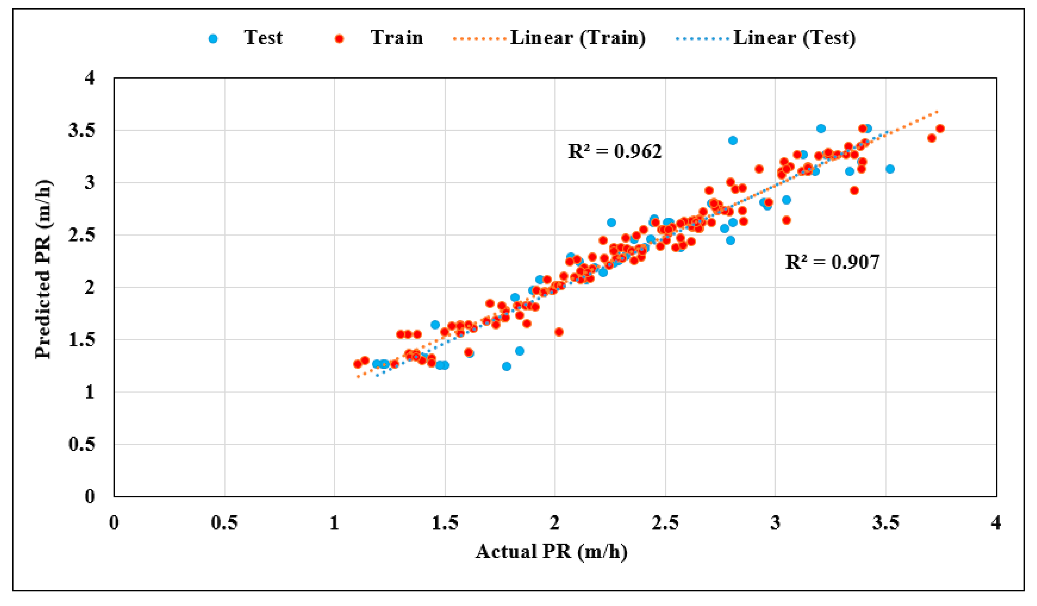
| KNN | TS | 0.907 | 0.204 | 89.574 | 0.157 | 0.944 | 3 | 3 | 3 | 3 | 4 | 16 |
| TR | 0.962 | 0.116 | 96.226 | 0.081 | 0.993 | 5 | 5 | 5 | 5 | 5 | 25 | |
| CART | TS | 0.897 | 0.216 | 88.020 | 0.164 | 0.944 | 2 | 2 | 2 | 2 | 4 | 12 |
| TR | 0.944 | 0.144 | 94.265 | 0.104 | 0.993 | 4 | 4 | 4 | 4 | 5 | 21 | |
| CHAID | TS | 0.850 | 0.252 | 83.838 | 0.179 | 0.944 | 1 | 1 | 1 | 1 | 4 | 8 |
| TR | 0.934 | 0.153 | 93.389 | 0.110 | 0.980 | 2 | 3 | 2 | 3 | 3 | 13 |
| NN | SVM | KNN | CART | CHAID | |
|---|---|---|---|---|---|
| Grand total rank | 31 | 37 | 41 | 33 | 21 |
| Input Variable | Importance |
|---|---|
| RPM | 0.14 |
| WZ | 0.15 |
| BTS | 0.16 |
| RQD | 0.17 |
| TF | 0.18 |
| UCS | 0.20 |
© 2019 by the authors. Licensee MDPI, Basel, Switzerland. This article is an open access article distributed under the terms and conditions of the Creative Commons Attribution (CC BY) license (http://creativecommons.org/licenses/by/4.0/).
Share and Cite
Xu, H.; Zhou, J.; G. Asteris, P.; Jahed Armaghani, D.; Tahir, M.M. Supervised Machine Learning Techniques to the Prediction of Tunnel Boring Machine Penetration Rate. Appl. Sci. 2019, 9, 3715. https://0-doi-org.brum.beds.ac.uk/10.3390/app9183715
Xu H, Zhou J, G. Asteris P, Jahed Armaghani D, Tahir MM. Supervised Machine Learning Techniques to the Prediction of Tunnel Boring Machine Penetration Rate. Applied Sciences. 2019; 9(18):3715. https://0-doi-org.brum.beds.ac.uk/10.3390/app9183715
Chicago/Turabian StyleXu, Hai, Jian Zhou, Panagiotis G. Asteris, Danial Jahed Armaghani, and Mahmood Md Tahir. 2019. "Supervised Machine Learning Techniques to the Prediction of Tunnel Boring Machine Penetration Rate" Applied Sciences 9, no. 18: 3715. https://0-doi-org.brum.beds.ac.uk/10.3390/app9183715