Discrete Element Analysis of Indirect Tensile Fatigue Test of Asphalt Mixture


1
School of Traffic and Transportation Engineering, Changsha University of Science and Technology, 960, 2nd Section, Wanjiali South RD, Changsha 410114, China
2
State Engineering Laboratory of Highway Maintenance Technology, Changsha University of Science and Technology, 960, 2nd Section, Wanjiali South RD, Changsha 410114, China
3
China Railway Major Bridge Reconnaissance & Design Institute Co., Ltd., 34, Hanyang RD, Wuhan 430050, China
*
Author to whom correspondence should be addressed.
Appl. Sci. 2019, 9(2), 327; https://0-doi-org.brum.beds.ac.uk/10.3390/app9020327
Submission received: 3 December 2018
/
Revised: 3 January 2019
/
Accepted: 7 January 2019
/
Published: 17 January 2019
(This article belongs to the Special Issue Achievements and Prospects of Advanced Pavement Materials Technologies)
Abstract
:In order to investigate the damage to microstructure and some other micromechanical responses during a fatigue test on asphalt mixture, Particle Flow Code (PFC) was used to reconstruct a two-dimensional discrete element model of asphalt mixture, based on computed tomography (CT) images and image-processing techniques. The indirect tensile fatigue test of asphalt mixture was simulated with this image-based microstructural model, and verified in the laboratory. It was found that there were four stages during the fatigue failure: no crack, crack initiation, crack developing, and interconnected crack. Cracks mainly developed between the aggregate and asphalt mortar, near the loading axis. The corresponding stages of failure, the developing trend and the distribution characteristics of the cracks matched well with those in the laboratory test. Furthermore, the trends of both the time-load curve and time-displacement curve from the simulation test were also consistent with those from the experimental test. In short, the distribution characteristics of cracks and internal forces of asphalt mixture show that it is feasible to simulate the fatigue performance of the asphalt mixture by a discrete element method (DEM).
1. Introduction
The fatigue failure is one of the most common distresses in asphalt pavements [1]. The fatigue properties of asphalt mixture could be evaluated by an indirect tensile fatigue test [2]. At present, the fatigue test of asphalt mixture is mainly carried out in the laboratory. However, the variability of asphalt mixture is very difficult to control during a laboratory test. Because of its heterogeneity, the fatigue properties are impossible to be fundamentally explored and evaluated by the laboratory test. Therefore, it is necessary to find a way to study the behavior and mechanism of the fatigue failure based on a more non-uniform microstructure [3].
Numerical simulation analysis is frequently used to study the micromechanical properties of the asphalt mixtures. Recently, some researchers have been trying to use a discrete element method (DEM) to analyze the fatigue properties of asphalt mixtures. Ma et al. analyzed the impacts of different parameters of air voids on the creep behavior of an asphalt mixture by the DEM [4,5]. Cao et al. conducted a two-point bending beam fatigue simulation test with the trapezoidal samples. The relationship between the fatigue properties of a French high modulus asphalt mixture and the Burger’s parameters were investigated by the DEM [6]. Gao et al. analyzed the failure procedure of an asphalt mixture by the DEM [7]. A local discrete element model was established to discuss the damage and cracks caused by the cyclic fatigue load [8]. Yu analyzed the effect of the aggregate packing on the dynamic modulus of an asphalt mixture by the DEM [9]. These achievements mentioned above demonstrate that the DEM is applicable for the research on fatigue characteristics of pavement asphalt mixes. However, the discrete element models of asphalt mixtures are generated by computer algorithms, which are different from the actual microstructures. The distribution characteristics of cracks and internal forces of asphalt mixtures are also seldom described in the indirect tensile fatigue test.
Since microstructure images captured by X-ray computed tomography (X-ray CT) can show the internal distribution and composition of the material, CT and the DEM have been widely applied to asphalt mixture together recently. You et al. obtained the images of asphalt mixture samples by the optical scanning, and reconstructed two-dimensional discrete element models based on these optical images [10]. Based on many two-dimensional slices of the same sample, the three-dimensional discrete element model of an asphalt mixture was reconstructed [11,12]. Zelelew et al. described the microstructure of asphalt mixtures obtained by CT and established a two-dimensional discrete element model to predict the creep compliance of uniaxial loading [13]. Zhou investigated the dynamic deformation process of an asphalt mixture based on the image-based discrete element model [14]. Tan believed that image-based discrete element model could provide a potential detailed insight into the failure mechanism of the heterogeneous rocks at the microscopic level [15]. Generally speaking, the asphalt mixture is a non-uniform complex viscoelastic material. It can be simulated more accurately by the DEM with CT image-based microstructural modeling. Therefore, the CT image-based microstructural modeling is feasible to simulate the asphalt mixture.
Therefore, in this paper, the two-dimensional discrete element model was reconstructed by the Particle Flow Code (PFC) software, based on the CT images. The indirect tensile fatigue simulation test was carried out to analyze the fatigue properties of the asphalt mixtures. The distribution of internal forces, damage to the microstructure, and some other micromechanical responses in the model were investigated. Furthermore, the simulation test was verified by the laboratory fatigue test.
2. Materials and Methods
2.1. Materials
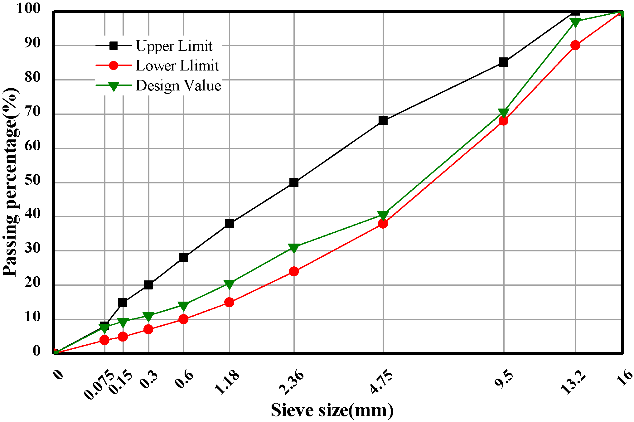
AC-13 asphalt mixture was designed according to JTG F40-2004 [16]. Figure 1 shows mix grading with upper and lower limits. The binders used the styrene-butadiene-styrene (SBS) modified asphalt, is the most common binders used in asphalt pavement [17,18]. Both the coarse and fine aggregates were basalt, and the filler was limestone. Experimental tests are carried out to evaluate the properties, they meet the requirement of the specification [19]. According to the Marshall method [20], the optimum asphalt content was 5.2%, and the filler content was 7%. Samples, with a diameter of 101.6 mm and height of 63.5 ± 1.3 mm, were compacted 75 times on each side according to JTG F40-2004 [16].
2.2. Methods
An image-based model was reconstructed by the DEM, and the discrete element analysis of an indirect tensile fatigue test was carried out. The distribution of the cracks and other simulation test results of the asphalt mixtures were validated by the laboratory test. The steps of the methodology are shown in Figure 2.
2.2.1. Discrete Element Analysis of the Indirect Tensile Fatigue Test
(1) Reconstruction based on the computed tomography (CT) images
Four Marshall samples were compacted in the laboratory. In order to distinguish among the aggregate particles, mortar and voids, an X-ray CT was used to obtain the images of the internal cross-sections of the samples. These images can be transferred to the model geometry in PFC2D. One of the sections at the height of 10–50 mm is present in Figure 3a. The aggregate, asphalt mortar and air voids in the CT image were separated by the image-processing technique. The image was converted to a binary format, in other words, the image was in the form of a digital matrix (from 0 to 255). Then image pixels became the particles in the PFC2D model. The position and geometric information of each phase were introduced into PFC in the form of coordinates, to reconstruct the model. Because of the accuracy and efficiency of calculation, the radius of the particle in the model was set at 0.75 mm, and the discrete element model is illustrated in Figure 3b.
(2) Micromechanical parameters
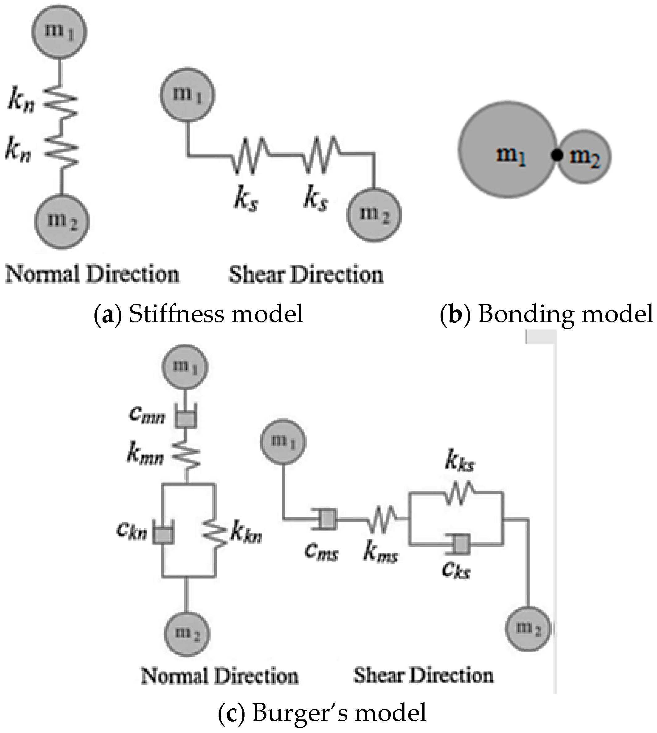
In this paper, the Burgers’ model was utilized to describe the properties of the contacts between the aggregate and asphalt mortar. Because the aggregates were all covered by the asphalt mortar, the contacts between different aggregates were ignored. The schematic diagrams of different contact models are shown in Figure 4. Different contact models between the different particles are present in Table 1. According to the micromechanical parameters in the paper of Feng [21] and Zelelew [13], the model parameters were set based on empirical values [22] and previous experimental results [5,23]. The parameters were also adjusted appropriately to match the experimental results of the indirect tensile test from the laboratory, i.e., peak force and stiffness. The parameters of the Burger’s model are shown in Table 2, the normal stiffness kn and the shear stiffness ks of each phase are illustrated in Table 3. The damp and calculating time-step of the model was a default value.
(3) Fatigue load and boundary conditions
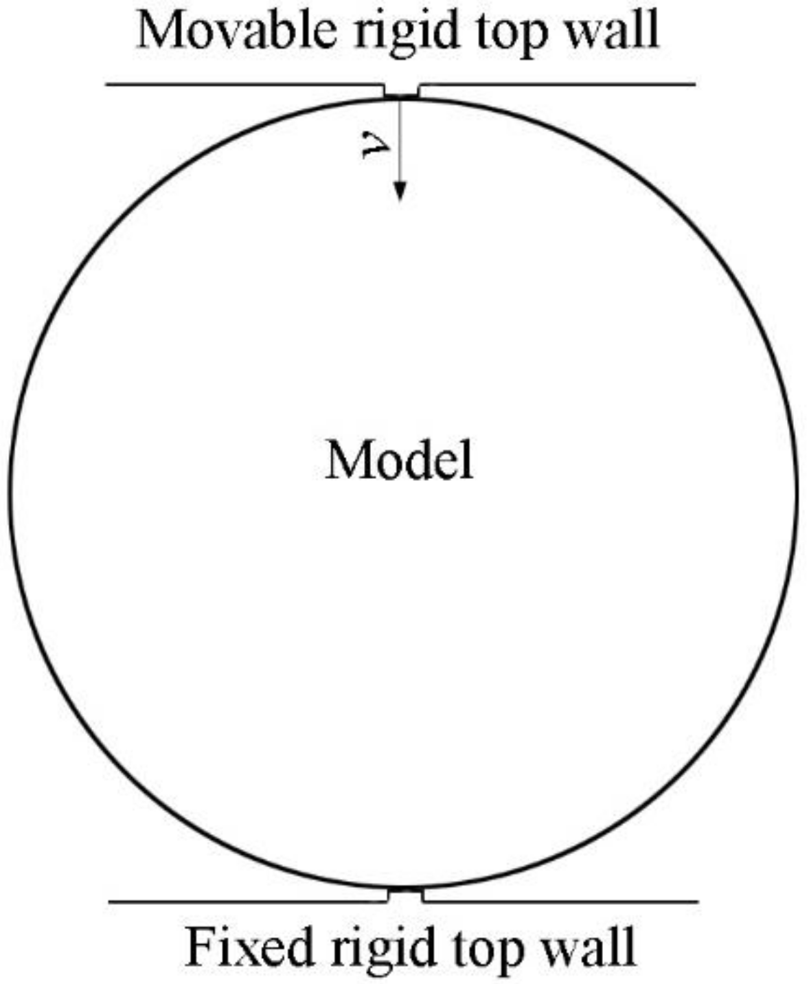
Two rigid walls were set at the top and bottom of the model (as shown in Figure 5). A stress-control mode was used in the simulation test, which was in accordance with the laboratory test. The rigid bottom wall of the model was fixed. In PFC2D, walls are assigned at constant or variable velocity. The variable speed of the top wall can be regulated by writing a servocontrol code. The displacement of the rigid top wall of the model was the vertical deformation of the model. The total stiffness of the particles was updated at each time-step. The multiplication of the total stiffness and the vertical deformation was the load on the model. In each cycle, the moving speed of the top wall could be back-calculated by the target load and stiffness. The speed of the top wall was controlled by the continuous sinusoidal load function. Its frequency was 10 Hz. The unbalanced force collected from the top wall was the fatigue load of the simulation test.
2.2.2. Experimental Test Validation in the Laboratory
To compare and analyze the distribution and development characteristic of the cracks, the indirect tensile fatigue test at the stress level of 0.7 was carried out. Samples with a diameter of 101.6 mm and height of 63.5 ± 1.3 mm were compacted using the Marshall method.
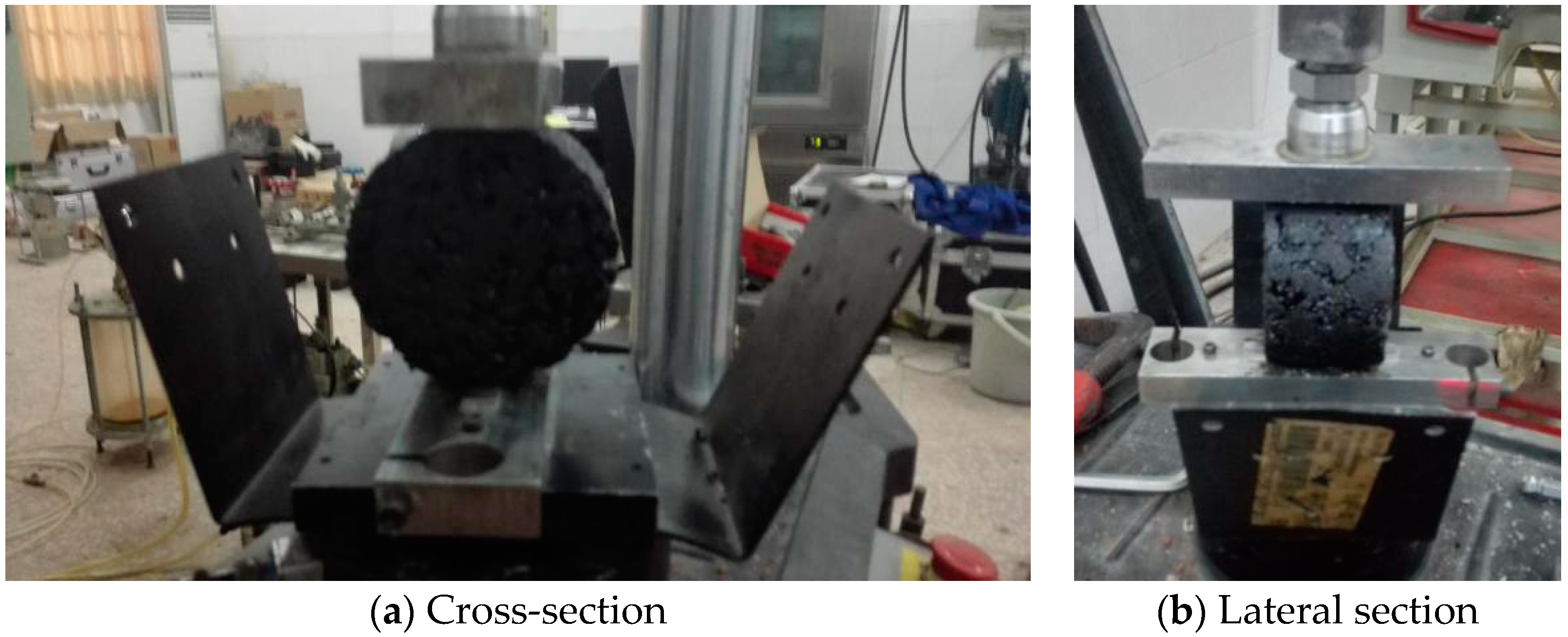
The indirect tensile fatigue test was carried out with an electro-hydraulic closed-loop servo MTS810 (as shown in Figure 6) material test system. The fixture was designed for the indirect tensile test. The width of the loading bar was set for 12.7 mm. In the indirect tensile fatigue test, the stress control mode was adopted, the load was subjected to a continuous semi-positive wave load, and the load level was determined by 0.7 of the indirect tensile strength.
3. Results and Discussions
3.1. Discrete Element Analysis of Indirect Tensile Fatigue Test
The fatigue simulation test has a high requirement for computer performance. The lower the stress level of the fatigue test, the longer the fatigue life the sample will have. In this case, each simulation loading cycle will take about one hour. When the stress level is 0.7, the fatigue life of the sample is more than 300 cycles, which takes about 300 h to calculate on the computer. Therefore, the stress level was set as 0.9 in these simulation tests to reduce the calculating time. The internal forces distribution, contact condition and displacement of the particle during the fatigue simulation test would be analyzed. The simulation test was divided into four stages: no crack, crack initiation, crack development and interconnected crack.
3.1.1. No Crack
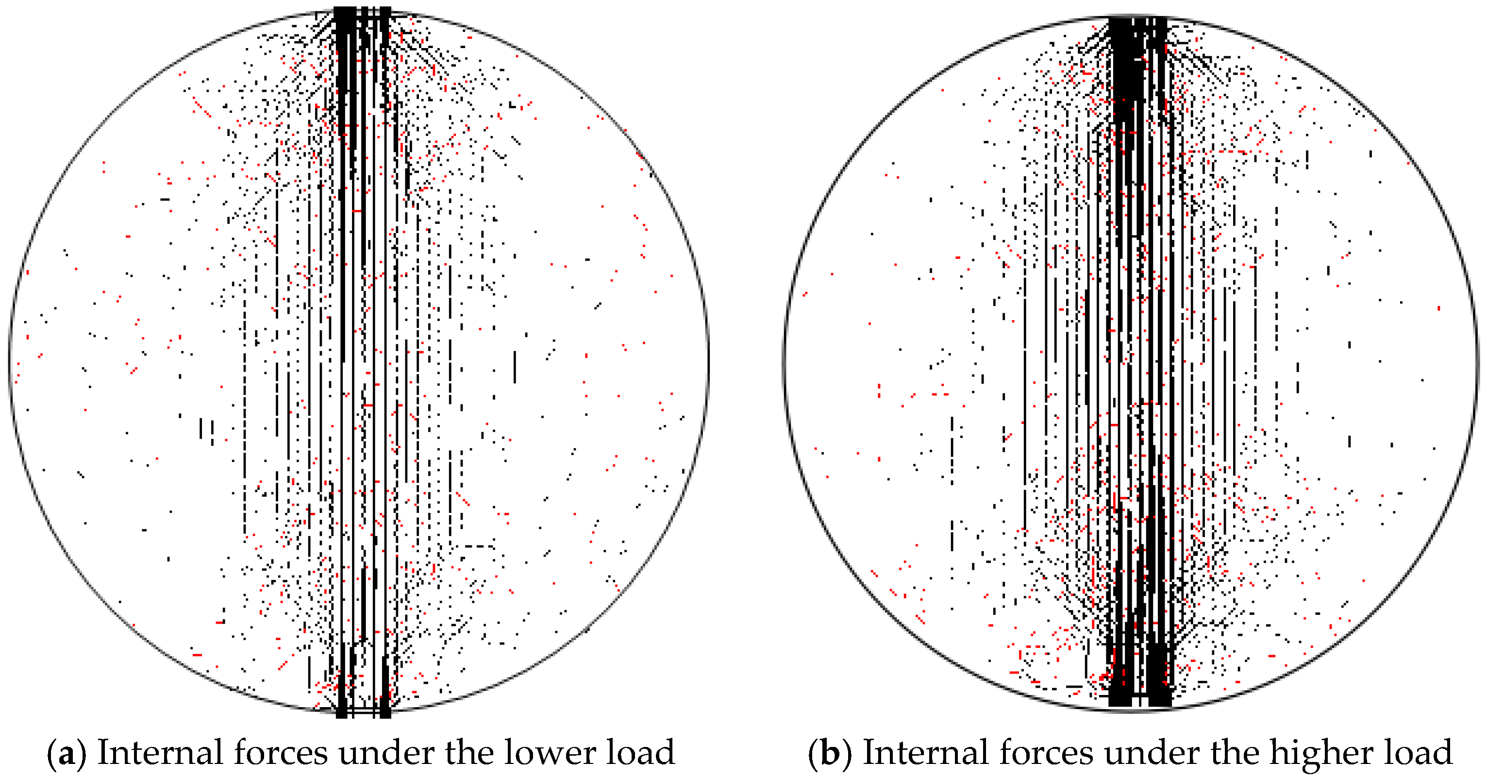
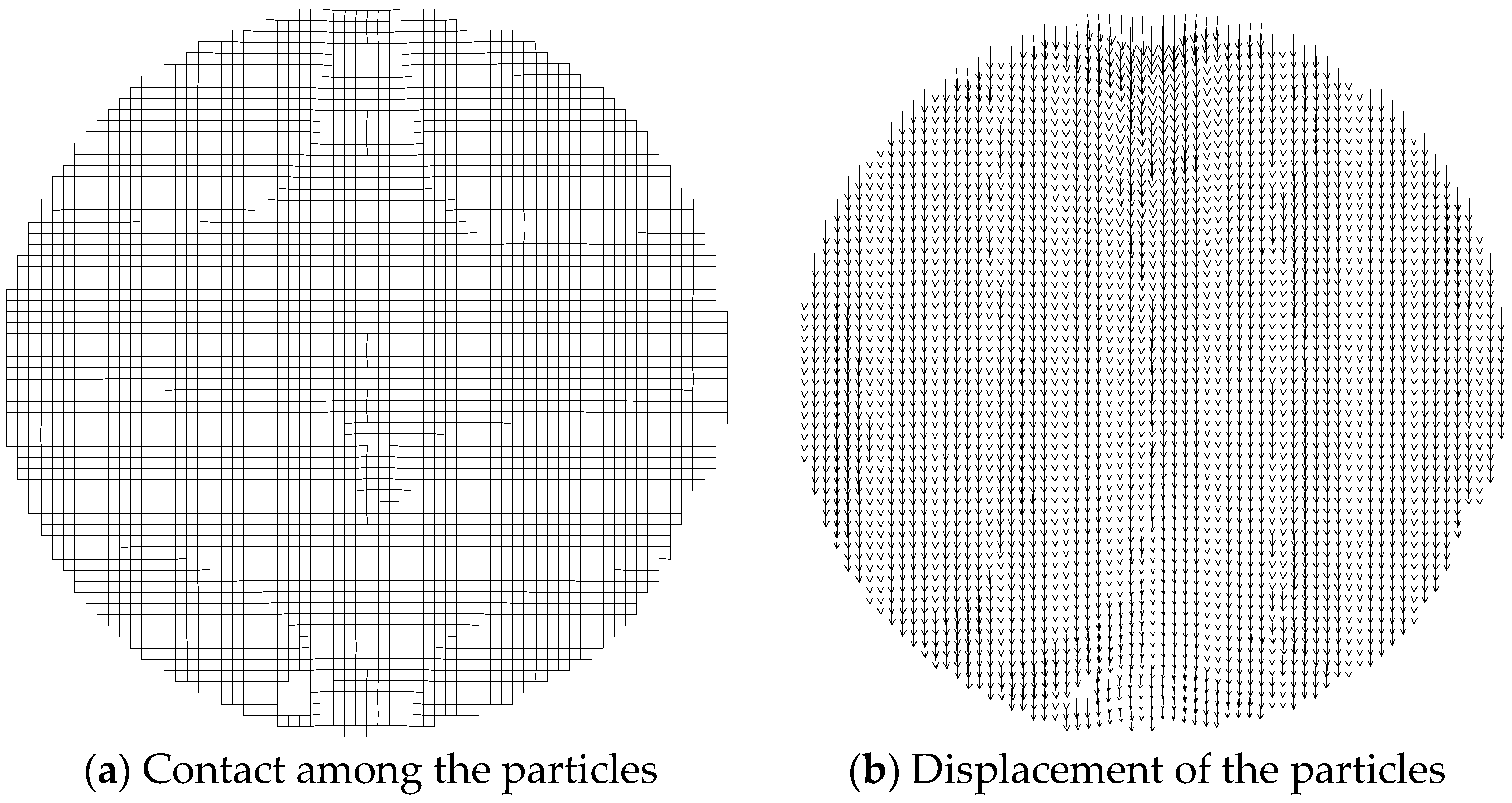
At the early loading stage, the internal force distribution of the model under two different loads is shown in Figure 7a,b. The black chain and red chain in the model are the compression and tension, respectively. Contacts and displacement of particles at early loading stage are illustrated in Figure 8.
- (1)
- From Figure 7, it can be found that internal forces mainly concentrate along the loading axial at the early loading stage. The forces on the bottom and top are bigger, but the forces in the center are smaller. After loading for a while, the force of the center increases, which means the forces are transferred from the top and bottom to the center of the sample.
- (2)
- In Figure 8, although almost all the particles in the model move downward, the contacts among the particles are good, and no crack appears. Moreover, the displacement near the top wall is the biggest, while the displacement near the bottom wall is the smallest.
3.1.2. Crack Initiation
- (1)
- According to Saint Venant’s principle, the transverse tensile forces will come out when the internal forces spread from the top and the bottom of the model to the whole cross-section under the fatigue load [24]. The thicker red force chain appears near the top wall at this stage, as shown in Figure 9a. Those mean that there are more significant tensile forces at the top of the model.
- (2)
- (3)
According to the analysis of the displacement and the forces distribution, it can be found that the crack is a kind of tensile force failure caused by the tensile stress; under the effect of the repeated transverse tensile forces, the contacts among the particles fail, and the cracks initiate.
3.1.3. Crack Development
After loading for a while, the crack develops downwards continually. This is at the crack development stage.
- (1)
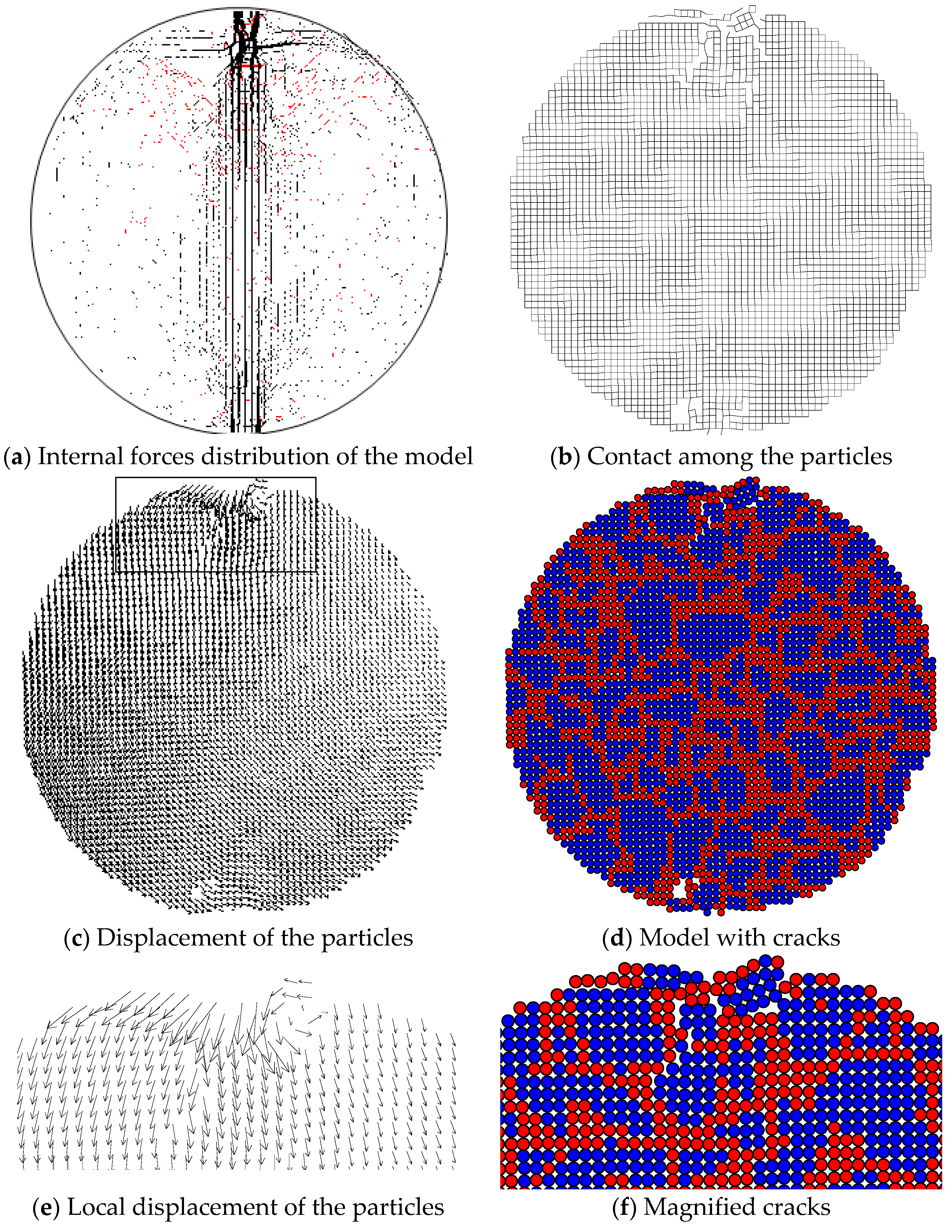
- From the forces distribution in Figure 10a. The chains, especially the red force chains, also continue to move downward, the black force chains change from the linear force chains with a uniform distribution to the curve force chains with the non-uniform distribution.
- (2)
- From the contact condition of the particles in Figure 10b, it can be found that the contact failure mainly distributes linearly near the top wall. This means that the cracks are mostly near the loading axis which connects the top wall.
- (3)
- In Figure 10d, there is displacement in different directions. In addition, there is also plenty of displacement in the same direction and different magnitudes.
Based on the internal forces, crack and displacement, it can be found that besides the failure of the tensile forces, there is also shear failure caused by inhomogeneous compressive forces in the model at this stage. Because of the high stiffness and strength of the aggregates, the cracks primarily come out at the interface between the aggregate and asphalt mortar [22].
3.1.4. Interconnected Crack
- (1)
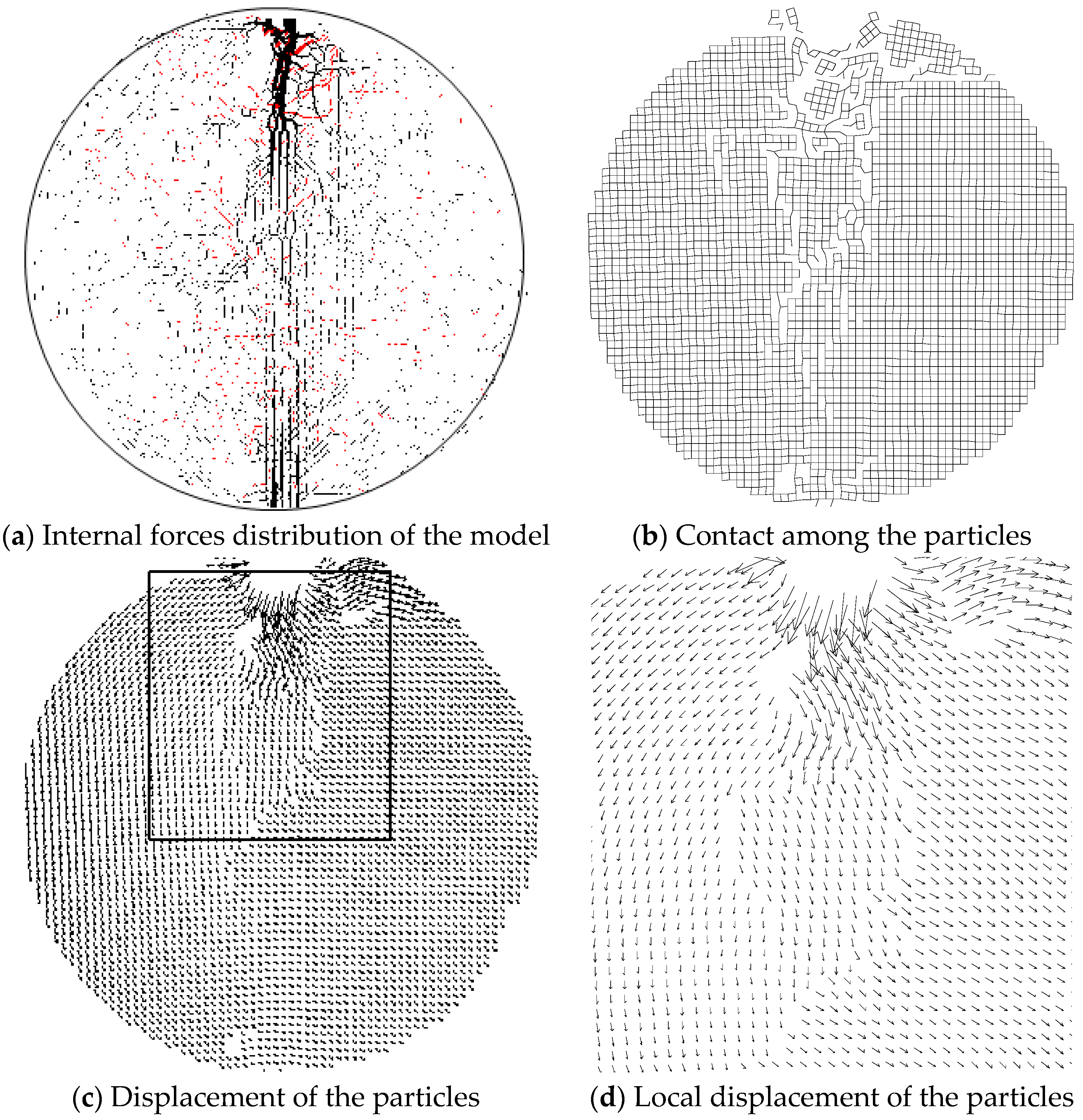
- When the cracks are interconnected, the forces distribution is present in Figure 11a. The internal forces are mainly near the loading axis. There are more intensive tensile forces and compressive forces where the contact fails, and the tensile forces are primarily at the top of the model.
- (2)
- The distribution of the cracks is given in Figure 11b; it is found that the cracks are also mainly near the loading axis. Only a few small cracks at the top of the model develop towards both sides of the model. The cracks primarily come out within the asphalt mortar or extend downwards along the interface between the aggregate and asphalt mortar.
- (3)
- From the displacements of the particles in Figure 11c,d, it is found that the displacement at different directions and displacement in the same direction come out in the model at the same time.
According to the distribution of the force and displacement of the particles, it is found that the forces failure and shear failure happen simultaneously during the failure process. This failure is mainly caused by the shear failure during the latter process. The tensile failure occurs under the repeated transverse tensile forces, and the cracks come out. Under the comprehensive effect of the non-uniform compressive forces and intensive tensile forces, the cracks develop downwards along the interface between the aggregate and asphalt mortar.
3.2. Experimental Test Validation in the Laboratory
The indirect tensile fatigue test at a low-stress level will need too much time, while the samples at the high-stress levels will break quickly. Although the fatigue life is different at different stress levels, the internal stress-strain responses of the model and development process of the crack are similar. Therefore, to compare and analyze the distribution and development characteristic of the crack, the indirect tensile fatigue simulation test and laboratory test were carried out at the stress level of 0.9 and 0.7, respectively. The time-load curves were obtained by both the simulation test and the laboratory test at the stress level of 0.9.
3.2.1. Characteristics of the Crack
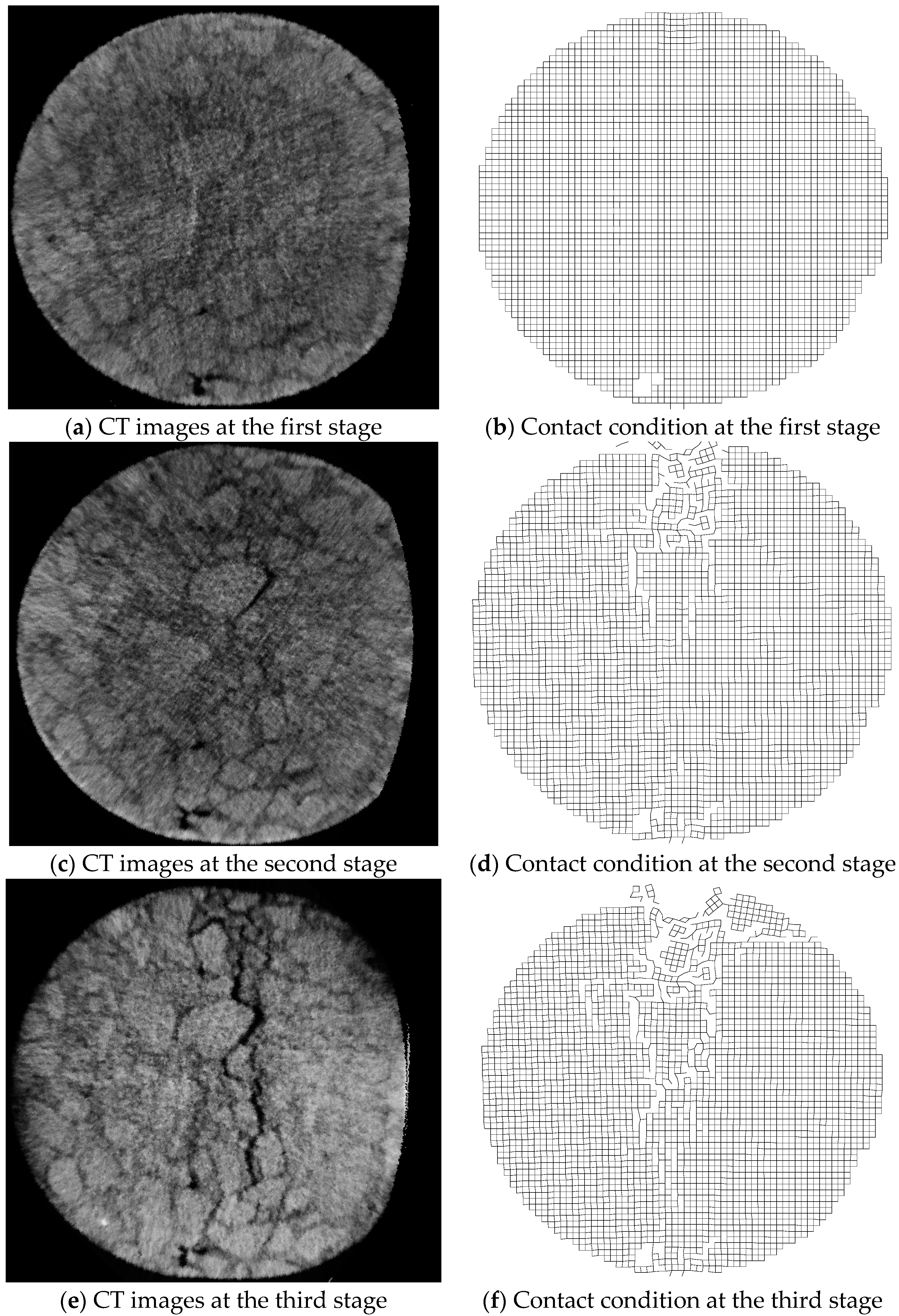
The samples were loaded at several stages. At each stage, the vertical deformation was controlled at 1.5 mm. After each loading stage, the sample was taken out for CT scanning. During the laboratory test, the samples were broken after three loading stages. The CT images at each stage were scanned and analyzed. The distribution and development characteristics of the crack from both simulation test and laboratory test were compared. The contact condition of the model and CT images at these three loading stages: no crack, crack developing, and crack interconnected are shown in Figure 12, respectively. In Figure 12, the CT images of the sample, acquired during the loading stages, are not perfect circles. Some part of the image on the right was missing because one X-ray tube of the CT was damaged. Since the cracks mainly distribute in the middle part of the section, the deficiency of the image can be ignored. According to the development and distribution characteristics of the crack at the three loading stages, the analysis is as follows:
- (1)
- At the first stage, when the vertical deformation of the sample is 1.5 mm, there is no crack in the CT image, as in Figure 12a. The stress is stable and there is no crack under the corresponding contact conditions in Figure 12b. It can be seen that the contacts among particles are intact. From the displacement of the particles in Figure 8c, it can be found that nearly all the particles move downwards under the load, which is in accordant with that in the laboratory test, for the sample is elastically compressed.
- (2)
- The fatigue loading stop after the top wall has moved downwards at the second 1.5 mm. In Figure 12c, the cracks have extended to the middle of the section, and the length is about 50 mm. Most of the cracks distribute near the loading axis of the section. From Figure 12d, it can be found that the contacts within the asphalt mortar, which is near the top wall or the loading axis, are completely damaged. According to Figure 12c,d, the length and distribution of the cracks are consistent.
- (3)
- After loading continually for a while, the cracks continue developing downwards until the main crack is interconnected. That is, the sample is damaged. In Figure 12e, as compared with the former stage, the sample breaks and has lots of small discontinuous cracks. It may result from that that there are only a few aggregates in the top of the model, and the model cannot bear the load after the cracks are interconnected. A few small cracks develop towards two sides of the model, which may be caused by the small cracks near the top wall, because the small cracks will develop outwards under the tensile stress. From Figure 12e,f, it can be found that the shape, length and distribution of the cracks from the simulation test are consistent with those from the laboratory test.
- (4)
- From Figure 12a–f, it can be found that the development and distribution characteristics of the cracks of the sample in each loading stage are in accordance with those of the discrete element model. As far as the characteristics of the crack are concerned, the indirect tensile fatigue simulation test matches the indirect tensile fatigue laboratory test very well.
3.2.2. The Time-Load Curve and Time-Displacement Curve
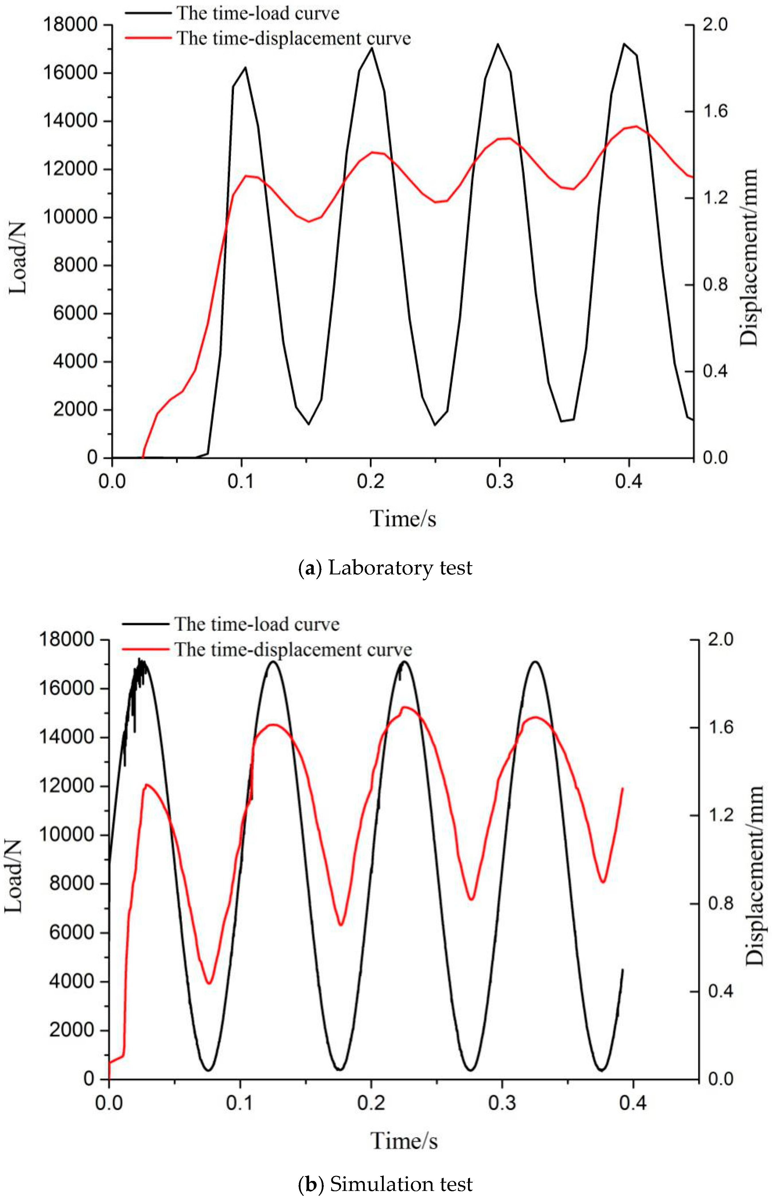
In the laboratory test, the load, loading time and vertical deformation of the sample were collected, and the time-load curve and time-displacement curve are plotted in Figure 13a. In the simulation test, the load is the unbalanced force received from the top wall. The loading time is the multiplication of the time-step length and the cycle times. The time-load curve and time-displacement curve of the simulation test are plotted in Figure 13b. Since the whole experiment would take too much time and produce lots of experimental data, only the first four cycles of the curve were compared between these two tests.
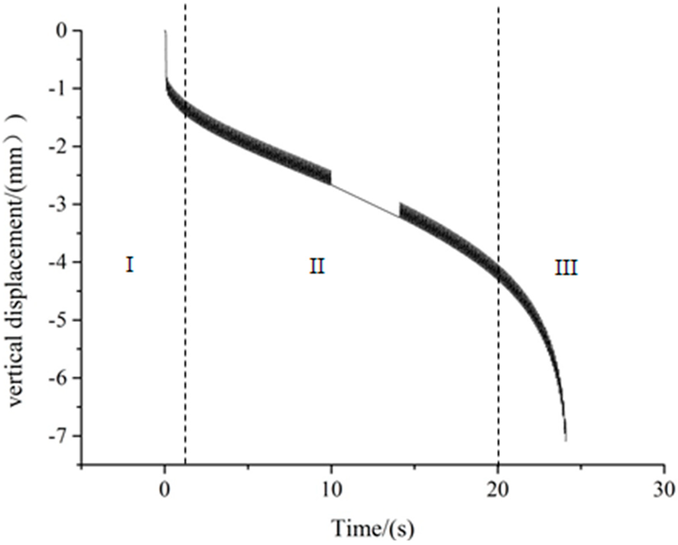
The loads of these two tests are both continuous sinusoidal loads. From the time-displacement curve in Figure 13, it can be found that the tendency of the vertical deformation in both tests is consistent: (1) the elastic deformation comes out under the sinusoidal load. The elastic deformation follows the sinusoidal law, just like the load. (2) The plastic cumulative deformation also occurs at the same time. The time-displacement curve of the model is a rising sinusoidal curve. Firstly, the bottom value of the sinusoidal curve increases rapidly after loading. When the stress becomes stable, it tends to be relatively flat. After the model breaks, it grows again quickly. In the laboratory test, just like the simulation test, the vertical deformation of the sample also can be divided into three stages: growing rapidly, relatively flat, and growing rapidly, as illustrated in Figure 14. Therefore, the stress-strain response of the simulation test is consistent with that of the laboratory test.
4. Conclusions
In this paper, the discrete element model was reconstructed based on the CT image of an actual sample, and an indirect tensile fatigue simulation test was carried out. The distribution characteristics of the cracks and internal forces in the simulation test were verified in the laboratory. The following conclusions can be drawn:
- (1)
- At the beginning of the loading, the internal forces of the model came down from the top of the model. The contacts among the particles were intact. The structure of the model was complete and there was not any crack. When the cracks came out, the contacts among the particles near the top wall were damaged first, and the particles with damaged contacts moved towards both sides of the crack. The failure here was caused by the tensile forces.
- (2)
- The model was loaded continually after cracking, and the particles whose contacts were damaged moved either to the different directions or the same direction with different distances. It was found that the cracks developed from the shear failure under the non-uniform compressive forces and the tensile failure under the intensive tensile forces.
- (3)
- When the model was damaged, the contact failure mainly happened near the loading axis of the model. The damaged contacts came out between the aggregates and asphalt mortar. The displacement at different directions and in the same direction was produced at both sides of the cracks. During the failure process, the shear failure and tensile failure co-occurred, but later development of the crack was mainly caused by the tensile failure.
- (4)
- The corresponding stages of the fatigue failure, development and distribution of the cracks, time-load curve and time-displacement curve of the indirect tensile fatigue simulation test were consistent with those of the laboratory test. That is, the applicability and feasibility of the fatigue simulation test were verified by the experimental test.
Author Contributions
Conceptualization, X.L. (Xuelian Li) and X.L. (Xinchao Lv); Methodology, X.L. (Xuelian Li); Software, X.L. (Xueying Liu); Resources, X.L. (Xuelian Li); Data Curation, X.L. (Xinchao Lv); Writing—Original Draft Preparation, X.L. (Xinchao Lv); Writing-Review & Editing, X.L. (Xuelian Li); Visualization, J.Y.; Project Administration, X.L. (Xuelian Li); Funding Acquisition, X.L. (Xuelian Li).
Funding
This work was funded by the National Natural Science Foundation of China [number 51308075], Department of Transport of Hainan Province (Number JT20160898009), and Open Fund of State Engineering Laboratory of Highway Maintenance Technology (Changsha University of Science & Technology) [number kfj160101, kfj140104].
Acknowledgments
Our special thanks go to all the subjects who participated in the data acquisition.
Conflicts of Interest
The authors declare no conflict of interest.
References
- Zhang, Y.; Luo, R.; Lytton, R.L. Mechanistic Modeling of Fracture in Asphalt Mixtures under Compressive Loading. J. Mater. Civ. Eng. 2012, 25, 1189–1197. [Google Scholar] [CrossRef]
- Said, S.F.; Vieira, J.M.; Hakim, H.; Eriksson, O.; Nilsson, R.; Cocurullo, A. Interlaboratory experiment of asphalt concrete using indirect tensile fatigue test. In Proceedings of the 5th Eurasphalt & Eurobitume Congress, Istanbul, Turkey, 13–15 June 2012. [Google Scholar]
- Chen, J.; Zhang, M.; Wang, H.; Li, L. Evaluation of thermal conductivity of asphalt concrete with heterogeneous microstructure. Appl. Therm. Eng. 2015, 84, 368–374. [Google Scholar] [CrossRef]
- Ma, T.; Zhang, D.; Zhang, Y.; Zhao, Y.; Huang, X. Effect of air voids on the high-temperature creep behavior of asphalt mixture based on three-dimensional discrete element modeling. Mater. Des. 2016, 89, 304–313. [Google Scholar] [CrossRef]
- Ma, T.; Zhang, Y.; Zhang, D.; Yan, J.; Ye, Q. Influences by air voids on fatigue life of asphalt mixture based on discrete element method. Constr. Build. Mater. 2016, 126, 785–799. [Google Scholar] [CrossRef]
- Cao, Q.; Liu, X.; Hao, W.; Huang, X.; Transportation, S.O.; University, S. Simulation and analysis of two-point bending fatigue test of asphalt concrete based on discrete element model. J. Southeast Univ. 2017, 33, 286–292. [Google Scholar]
- Gao, X.; Koval, G.; Chazallon, C. A discrete element model for damage and fracture of geomaterials under fatigue loading. In Proceedings of the 8th International Conference on Micromechanics on Granular Media, Montpellier, France, 3–7 July 2017. [Google Scholar]
- Gao, X. Modelling of Nominal Strength Prediction for Quasi-Brittle Materials: Application to Discrete Element Modelling of Damage and Fracture of Asphalt Concrete under Fatigue Loading. Ph.D. Thesis, University of Strasbourg, Strasbourg, France, 2017. [Google Scholar]
- Yu, H.; Shen, S. Impact of aggregate packing on dynamic modulus of hot mix asphalt mixtures using three-dimensional discrete element method. Constr. Build. Mater. 2012, 26, 302–309. [Google Scholar] [CrossRef]
- You, Z. Development of a Micromechanical Modeling Approach to Predict Asphalt Mixture Stiffness Using the Discrete Element Method. Ph.D. Thesis, University of Illinois at Urbana, Champaign, IL, USA, 2003. [Google Scholar]
- You, Z.; Adhikari, S.; Kutay, M.E. Dynamic modulus simulation of the asphalt concrete using the X-ray computed tomography images. Mater. Struct. 2009, 42, 617–630. [Google Scholar] [CrossRef]
- You, Z.; Buttlar, W.G. Discrete Element Modeling to Predict the Modulus of Asphalt Concrete Mixtures. J. Mater. Civ. Eng. 2004, 16, 140–146. [Google Scholar] [CrossRef]
- Habtamu, M.Z.; Athanassios, T.P. Micromechanical Modeling of Asphalt Concrete Uniaxial Creep Using the Discrete Element Method. Road Mater. Pavement Des. 2015, 11, 613–632. [Google Scholar]
- Ji, Z.; Qiong, T.; Yong-qin, R.; Hong, Y. A DEM Geometric Modeling Method of HMA Based on Digital Imaging Processing. J. Civ. Archit. Environ. Eng. 2012, 34, 136–140. [Google Scholar]
- Tan, X.; Konietzky, H.; Chen, W. Numerical Simulation of Heterogeneous Rock Using Discrete Element Model Based on Digital Image Processing. Rock Mech. Rock Eng. 2016, 49, 4957–4964. [Google Scholar] [CrossRef]
- Technical Specifications for Construction of Highway Asphalt Pavements; JTG F40-2004; China Communications Press: Beijing, China, 2004.
- Behnood, A.; Gharehveran, M.M. Morphology, rheology, and physical properties of polymer-modified asphalt binders. Eur. Polym. J. 2018. [Google Scholar] [CrossRef]
- Li, X.; Zhou, Z.; You, Z. Compaction temperatures of Sasobit produced warm mix asphalt mixtures modified with SBS. Constr. Build. Mater. 2016, 123, 357–364. [Google Scholar] [CrossRef]
- Test Methods Aggregate of Highway Engineering Aggregate; JTG E42-2005; China Communications Press: Beijing, China, 2005.
- Application Handbook of Standard Test Methods of Bitumen and Bituminous Mixtures for Highway Enginerring; JTG E20-2011; China Communications Press Co., Ltd.: Beijing, China, 2011.
- Feng, H.; Pettinari, M.; Stang, H. Study of normal and shear material properties for viscoelastic model of asphalt mixture by discrete element method. Constr. Build. Mater. 2015, 98, 366–375. [Google Scholar] [CrossRef]
- Chen, J.; Zhang, D. Application of Particle Flow Code in Rode Engineering; China Communications Press Co., Ltd.: Beijing, China, 2015. [Google Scholar]
- Liu, X. The Research on Microscopic Mechanism of Top-Down Cracking in Asphalt Pavement. Master’s Thesis, Changsha University of Science & Technology, Changsha, China, 2017. [Google Scholar]
- He, Z.Q.; Liu, Z. Investigation of Bursting Forces in Anchorage Zones: Compression-Dispersion Models and Unified Design Equation. J. Bridge Eng. 2011, 16, 820–827. [Google Scholar] [CrossRef]
Figure 1.
Gradation of aggregate for asphalt mixture AC-13.

Figure 2.
Flowchart of steps of the test.

Figure 3.
The computed tomography (CT) image and the corresponding discrete element model.

Figure 4.
Schematic diagrams of different contact models.

Figure 5.
Boundary condition of the model.

Figure 6.
Indirect tensile fatigue test in the laboratory.

Figure 7.
Internal forces distribution at early loading stage.

Figure 8.
Model at early loading stage.

Figure 9.
Crack initiation.

Figure 10.
Crack development.

Figure 11.
Interconnected crack.

Figure 12.
Cracks in the simulation test and laboratory test.

Figure 13.
Time-load curves and time-displacement curves.

Figure 14.
Time-displacement curve of the sample in the laboratory test.


Table 1.
Contact models of the asphalt mixture.
| Contact Points | Contact Models |
|---|---|
| Between aggregates | Stiffness model + Bonding model |
| Within asphalt mortar | Stiffness model + Burger’s model + Bonding model |
| Between aggregate and asphalt mortar | Stiffness model + Burger’s model + Bonding model |
Table 2.
Micromechanical parameters of different contacts.
| Micro Parameters | kn | ks |
|---|---|---|
| Between aggregates | 4.2 × 10⁸ | 3.0 × 10⁷ |
| Within asphalt mortar | 6.3 × 10⁷ | 0.6 × 10⁷ |
Table 3.
Micromechanical parameters of Burger’s model.
| Parameters | Maxwell | Kelvin | ||
|---|---|---|---|---|
| Stiffness | Viscosity | Stiffness | Viscosity | |
| Normal | 6.04 × 10⁵ | 2.2 × 10⁷ | 1.33 × 10⁵ | 2.77 × 10⁶ |
| Tangential | 2.42 × 10⁵ | 8.81 × 10⁶ | 5.3 × 10⁴ | 1.11 × 10⁶ |
© 2019 by the authors. Licensee MDPI, Basel, Switzerland. This article is an open access article distributed under the terms and conditions of the Creative Commons Attribution (CC BY) license (http://creativecommons.org/licenses/by/4.0/).
Share and Cite
MDPI and ACS Style
Li, X.; Lv, X.; Liu, X.; Ye, J. Discrete Element Analysis of Indirect Tensile Fatigue Test of Asphalt Mixture. Appl. Sci. 2019, 9, 327. https://0-doi-org.brum.beds.ac.uk/10.3390/app9020327
AMA Style
Li X, Lv X, Liu X, Ye J. Discrete Element Analysis of Indirect Tensile Fatigue Test of Asphalt Mixture. Applied Sciences. 2019; 9(2):327. https://0-doi-org.brum.beds.ac.uk/10.3390/app9020327
Chicago/Turabian StyleLi, Xuelian, Xinchao Lv, Xueying Liu, and Junhong Ye. 2019. "Discrete Element Analysis of Indirect Tensile Fatigue Test of Asphalt Mixture" Applied Sciences 9, no. 2: 327. https://0-doi-org.brum.beds.ac.uk/10.3390/app9020327
Note that from the first issue of 2016, this journal uses article numbers instead of page numbers. See further details here.