Article

A Novel Plant Propagation-Based Cascaded Fractional Order PI Controller for Optimal Operation of Grid-Connected Single-Stage Three-Phase Solar Photovoltaic System

Department of Electrical Engineering, Inha University, 100, Inha-ro, Nam-gu, Incheon 402-751, Korea
*
Author to whom correspondence should be addressed.
Submission received: 30 August 2019 / Revised: 1 October 2019 / Accepted: 8 October 2019 / Published: 11 October 2019
(This article belongs to the Special Issue Computational Intelligence in Photovoltaic Systems - Volume II)

Abstract

:
Grid-connected photovoltaic (PV) inverters are gaining attention all over the world. The optimal controller setting is key to the successful operation of a grid-connected PV system. In this paper, a novel plant propagation algorithm-based fractional order proportional-integrator (FOPI) controller for cascaded DC link voltage and inner current control of a grid-connected PV controller has been proposed, which outperforms particle swarm optimization-based PI and elephant herding optimization-based FOPI in terms of multicriteria-based analysis. The performance of the proposed controller also has been measured in terms of total harmonic distortion to maintain the appropriate power quality. Also, the proposed controllers were tested under various solar irradiance and voltage sag conditions to show the effectiveness and robustness of the controllers. The whole system is developed in OPAL-RT using MATLAB/Simulink and RT-LAB as a machine-in-loop (MIL) system to validate the performance in real time.

1. Introduction

Grid-connected photovoltaic (PV) systems have acquired quite a good proportion of usage among different renewable energy sources. Every year, the amount of grid-feeding PV systems in use is increasing. As a result, it is becoming highly required that the grid-connected PV systems operate optimally to perform stable grid operation and meet user demand.
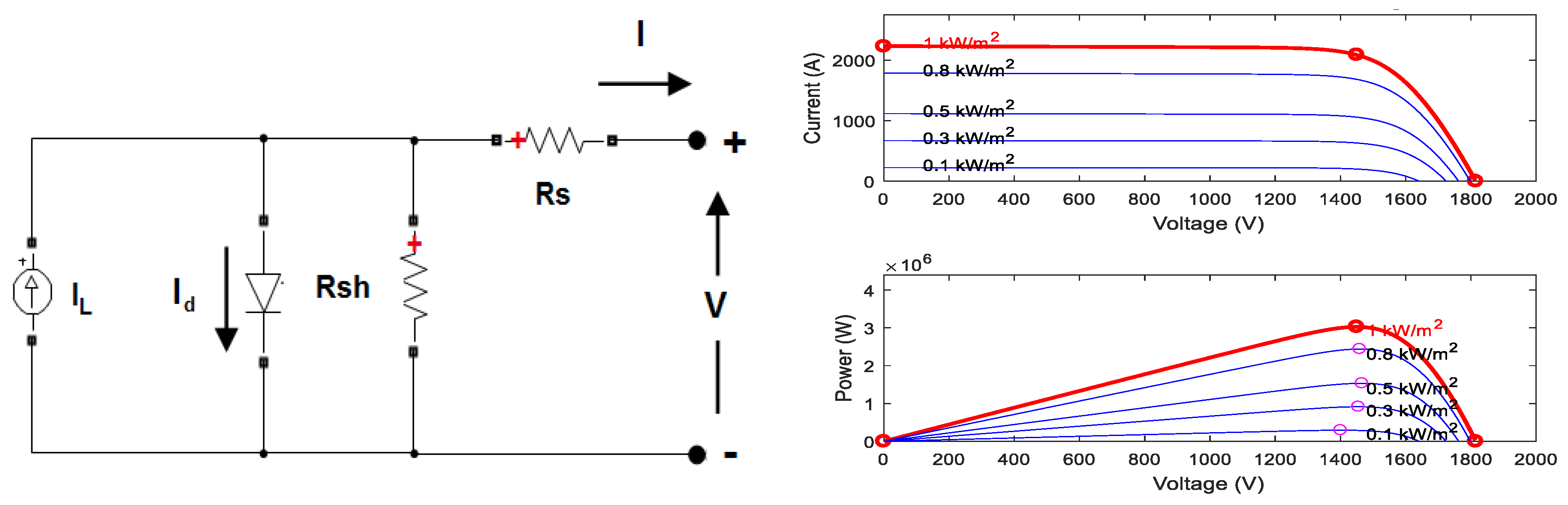
One of the primary models for grid-connected solar PV is single-stage model that uses only a single converter. Such converters either can be voltage source or current source inverters. The control of the converters requires inner current control loops and an outer voltage control loop. The reference of the outer voltage control loop can be found by maximum power point tracking (MPPT) technique, and the output of the voltage control loop can be used a reference for the inner current control loop. These controllers require tuning of their respective parameters for optimal operation of the system. Development of different controllers for optimal operation of grid-connected distributed generation or PV systems has been widely described in different literature. Touqeer et al. [1] proposed a grasshopper optimization algorithm-based optimal power flow controller for a grid-connected Distributed Generation (DG) system. The authors only tuned the outer control loop while keeping fixed internal loop values, which makes the system difficult to tune when the values of internal loop gain parameters are unknown. Sharifian et al. [2] proposed a reactive power control and adaptive predictive current control strategy, where the Reactive Power controller (RPC) generates the reactive current using a PI controller. Tafti et al. [3] proposed a three-level neutral point clamped inverter instead of a two-level Voltage Source Inverter (VSI) with voltage-oriented control strategy using proportional resonant (PR) controller. A fictitious reference iterative tuning method using particle swarm optimization for tuning a DC link voltage controller was proposed in [4]. In [5] authors discussed single-stage topology with a current source inverter (CSI) with MPPT and double tuned resonant filter. They also proposed series addition of a small DC link inductor with double-tuned resonant filter to eliminate harmonics. The authors used proportional resonant controller for voltage and current control loop. Touil et al. [6] proposed sliding mode control to force the output voltage of the PV and grid power factor to follow a certain trajectory reference. This requires rigorous calculation for determination of control law. Azghandi et al. presented a precise phasor model and employed an active power loop cascaded with an inner reactive power loop [7]. Few works also proposed methodologies to work under fault conditions. DC link voltage control of a grid-connected PV system with enhanced fault ride through capability enhancement was proposed by Mohamed et al. [8]. The proposed control scheme includes control without MPPT which activates when DC link voltage exceeds the nominal value. In [9], Khawla et al. proposed a three-phase grid-connected PV system working with MPPT and non-MPPT mode to work under grid fault mode. Recently, Islam et al. [10] designed a proportional resonant controller with resonant harmonic compensator for a grid-connected photovoltaic system. The authors have also proposed a switch-type fault current limiter for fault ride through a capability which can work under asymmetrical faults also.
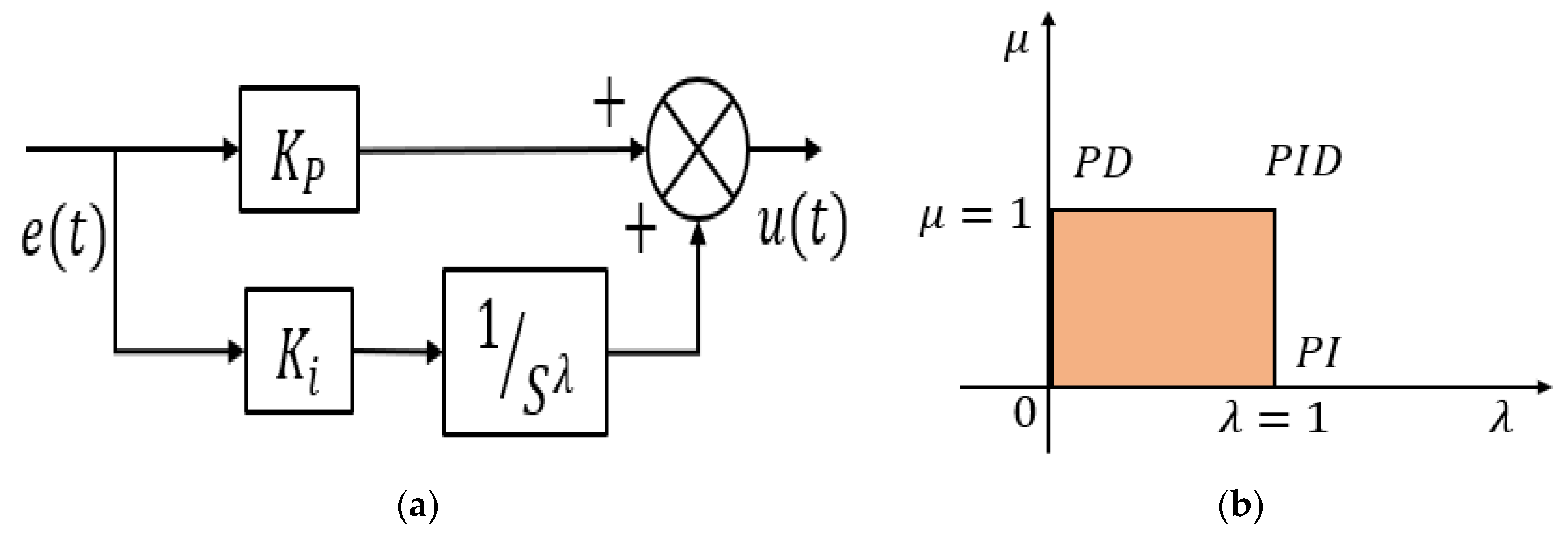
Although different methodologies have been proposed by different authors, almost all of them have considered the controllers with internal gain parameters; these works have rarely discussed any systematic approach for tuning of those parameters irrespective of the controller type, which is one of the most important issues while designing a successful controller. Because trial-and-error or Ziegler–Nichols methods often suffer from huge time consumption and optimal parameter selection uncertainty, it is highly required to discover a systematic optimal tuning process which can guarantee satisfactory results within minimum time and computation effort. Also, as the outer voltage control loop and the inner current loop are cascaded in nature, separate tuning will take time to get optimal results. Hence, simultaneous tuning is required to tune optimally. Moreover, the system response can be suboptimal when applying a conventional PI controller due to the fixed-order integrator. Hence the system can be more sophisticated by applying a well-tuned fractional order PI (FOPI) controller due to its capability of dealing with fractional order integrators. Again, this needs a systematic approach to tune the respective parameters.
Thus, in this work, a novel plant propagation algorithm (PPA)-based simultaneous and cascaded outer DC link voltage and inner current loop controller is proposed. The proposed method is applied with fractional order PI controller instead of the conventional PI controller due to its increase in degree of freedom to control more precisely. The considered objective function consists of two terms (integral of absolute time error and peak difference) which effectively reduces the overshoot, settling time and steady-state error if the controller is tuned properly. The proposed controller is also compared with two other metaheuristic algorithms, namely particle swarm optimization (PSO) and elephant herding optimization (EHO). Using PSO, conventional PI is tuned; using EHO, FOPI is tuned. The differences in results and reasonings are covered in detail to understand the science behind better results with PPA over PSO and EHO. As systems are becoming more and more digitized, the real-time simulation is also required to develop appropriate digital twins to emulate physical systems in the cyber domain. A successful development of an optimal controller in real-time simulators can lead to such achievements proficiently. Thus, the proposed controllers were tested in real-time simulator OPAL-RT. The performance of the proposed controller was also extended by analysis of the total harmonic distortion (THD) of the inverter current and performance during voltage sags and varied irradiance in grid-connected mode.
The paper is arranged in the following order. 
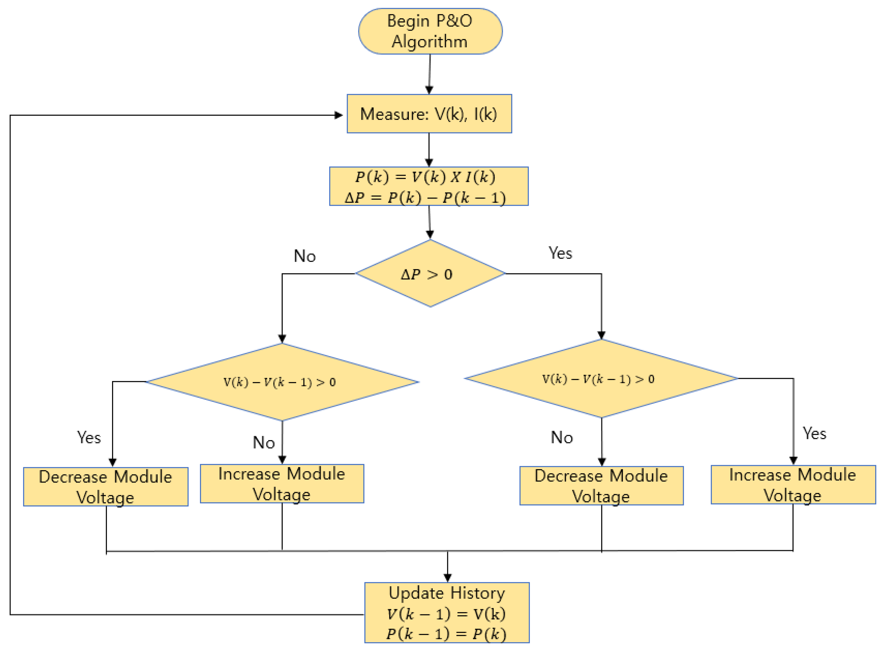
Section 2 describes the system, system components, and mathematical modeling of the considered system along with perturbation-and observation-based MPPT algorithm. In Section 3 the objective function, working flow chart, and algorithms are discussed in detail. Section 4 deals with the experimental setup, parameter selection, and simulation results. Analyses of results and comparative analysis of the experimented optimization methods are also covered in the same section. In Section 5, performance of the selected controller is also tested under varied conditions and in terms of THD criteria. Finally, Section 6 concludes and summarizes the paper with a direction to future prospective work.

2. System Modeling

Figure 1 depicts a conventional single-stage grid-connected PV system, which comprises PV panels, DC link capacitor, DC-to-AC inverter, RLC filter, transformer, and the main grid. The heart of this system is the inverter control section, which controls the inverter by controlling the gate pulses based on the MPPT and control loop techniques. In this work, we have considered the perturbation and observation-based MPPT technique to provide reference voltage for the DC link voltage controller, whereas DC link voltage controller output works as inner current control loop control reference (d-axis current). The q-axis current component reference can be set by setting reactive power requirements.

2.1. PV Panel

In this work, the help of MATLAB/Simulink SimPowerSystem toolbox is taken to use the PV panel. The PV module equivalent circuit and its I–V and P–V characteristics are shown in Figure 2.
The diode I–V characteristics for a single module are defined as [11]:
I d = I 0 [ e x p ( V d V T ) 1 ]
V T = k T q n I N c e l l
where, I d and V d are diode current and voltage, respectively. I 0 is diode saturation current. k , T , and q are Boltzmann constant, cell temperature in kelvin, and electron charge, respectively. n I and N c e l l are known as diode ideality factor and number of cells connected in series in a module, respectively.

2.2. Perturbation and Observation (P&O)-Based MPPT

In P&O technique [12] the tracker operates by periodically increasing or decreasing the voltage. The controller changes the reference voltage for the DC link voltage controller by tracking and comparing the present and one-step-behind power and voltage values. The increasing or decreasing of the reference value is applied with a fixed small value. The flowchart of a perturbation and observation-based algorithm is given below in Figure 3.

2.3. Outer Voltage Control Loop and Inner Current Control Loop

Figure 4 represents the outer voltage and inner current control loops, where, V d c and V d c are the reference voltage fed from MPPT controller and measured DC link voltage, respectively. Q g is the reference reactive power. i d g and i q g are the reference d- and q-axis current components of grid current, respectively. i d g and i q g are the measured d- and q-axis current components of grid current, respectively. V d g and V q g are d- and q-axis components of grid voltage.
R g and L g are resistance and the inductance values, respectively, of the filter and transformer. In general, transformer resistances and inductances are neglected in transformerless systems. But if the system size increases, the necessity of a transformer is inevitable for insulation between high-tension and low-tension sides. Hence the internal transformer impedances must be considered for proper values of PI controller tuning. Thus, the equation for R g and L g can be written as:
R g = R f + R x f ( p r i m a r y ) + R x f ( s e c o n d a r y )   and   L g = L f + L x f ( p r i m a r y ) + L x f ( s e c o n d a r y ) ,
where, z f refers to the filter component; z x f ( p r i m a r y ) and z x f ( s e c o n d a r y ) refer to components associated with the primary and secondary windings of a transformer, respectively. PI/FOPI controllers perform better in dq0 reference frame, hence abc components are converted to dq0 frame using the following relation [13]:
[ x d x q ] = 2 3 [ c o s θ c o s ( θ 2 π 3 ) c o s ( θ 4 π 3 ) s i n θ s i n ( θ 2 π 3 ) s i n ( θ 4 π 3 ) ] [ x a x b x c ] .
The reference value for the inner current control loop i d g and i q g can be found using:
i d g = ( K p V + K i V s ) ( V d c V d c ) ,
or
i d g = ( K p V + K i V s λ V ) ( V d c V d c )
and   i q g = Q g 3 2 V d g .
The nominal value of DC link voltage can be found using:
V d c = 6 V a m a ,
where V a is grid phase voltage and m a is the modulation index.
Considering the cross-decoupling terms, the inner loop equations can be written as:
V d i = ( K P I + K i I s ) ( i d g i d g ) ω g L g i q g + V d g + R g i d g ,
or
V d i = ( K P I + K i I s λ I ) ( i d g i d g ) ω g L g i q g + V d g + R g i d g
and
V q i = ( K P I + K i I s ) ( i q g i q g ) + ω g L g i q g + V q g + R g i q g ,
or
V q i = ( K P I + K i I s λ I ) ( i q g i q g ) + ω g L g i q g + V q g + R g i q g ,
where the indexes associated with the gain parameters ( K p X , K i X , and λ X ) represent the corresponding controller types such as voltage or controller. The objective of this work is to find the optimal values of such parameters for the optimal operation of the system. Due to the similar nature of Equations (7a) and (7b), in Equations (8a) and (8b) we can tune the controller with the same values for both d- and q-axis current control loop, which will reduce computational complexity and time to optimize.
The V d i and V q i are again converted into abc frame to control the gate pulses of the inverter using the following equation [13]:
[ x a x b x c ] = [ c o s θ s i n θ c o s ( θ 2 π 3 ) s i n ( θ 2 π 3 ) c o s ( θ 4 π 3 ) s i n ( θ 4 π 3 ) ] [ x d x q ] .
Equations (4b), (7b), and (8b) are an alternative form of Equations (4a), (7a), and (8a) in terms of the fractional order PI controller. The general block diagram and graphical representation of fractional order PI controller is as follows [14].
From Figure 5b, the difference of fractional order PID controller with the conventional PID controller is the presence of terms λ and μ . These parameters increase the degree of freedom and hence the controller performance improves depending on the type of system and problem in hand.

3. Objective Function

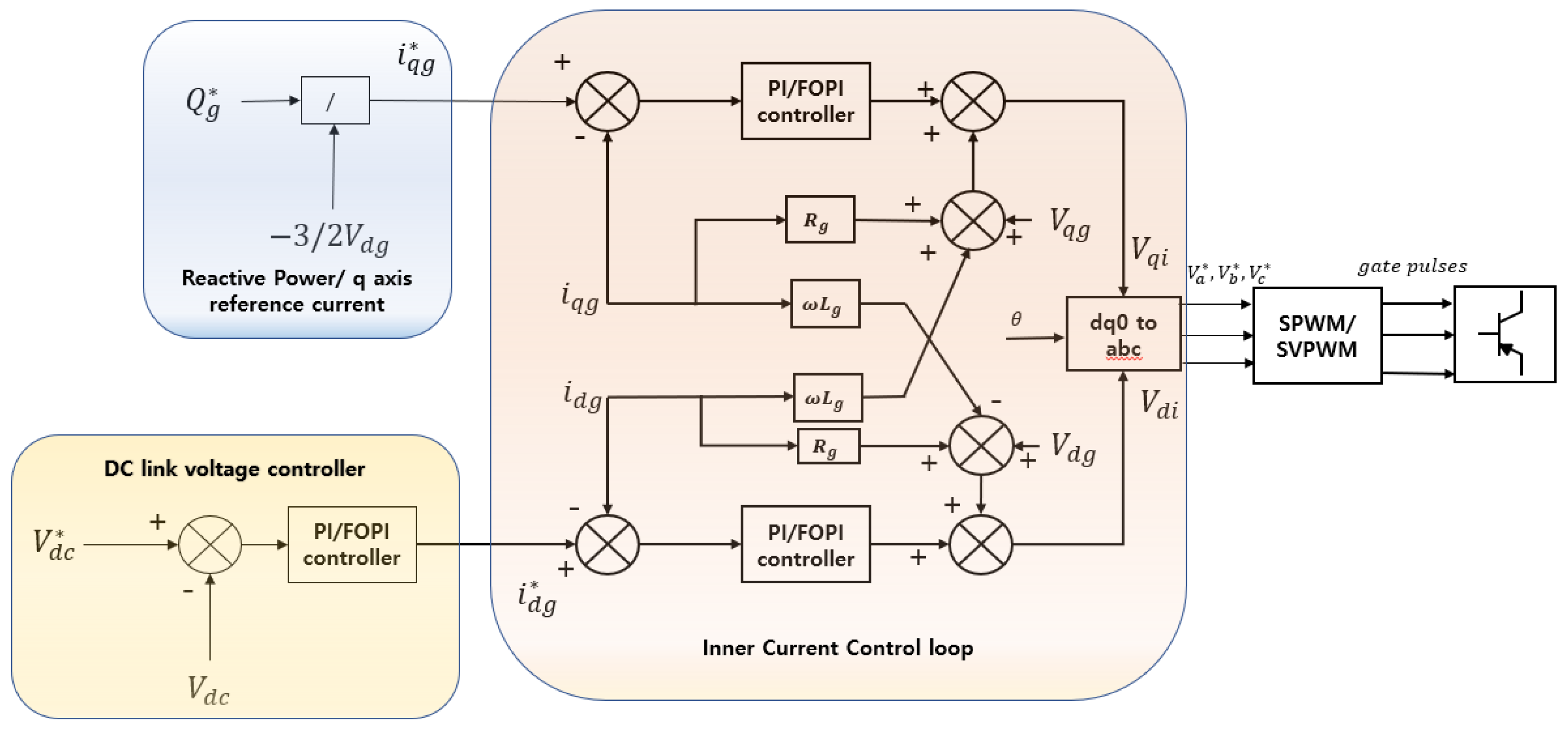
The system consists of cascaded outer voltage and inner d-axis current and reactive power/q-axis current control loops. Due to the cascaded nature of the control system, it is highly required that the inner loop of the designed controller must follow the outer loop with a minimum amount of error. Generally, the errors are calculated using four renowned methods known as IAE, ISE, ITSE, and ITAE [15]. IAE and ISE put equal importance on error irrespective of the time, but ITSE and ITAE put different weight on error with respect to time due to the presence of time in the objective function. In ITSE, due to presence of square term, error drops drastically as the error converges to zero. ITAE is free from such a problem, as it puts different weight to error with respect to time without squaring the error. However, only using such criterions sometimes does not guarantee lesser peak overshoot. Hence, a peak difference term is also added in the objective function to minimize the peak overshoot along with ITAE.
The proposed objective function is as follows:
= min ( P e a k   D i f f e r e n c e + 0 t s i m t | e ( t ) | d t ) ,
where
Peak   Difference = Peak   Value   of   the   response Reference   Value   or   final   value ,
and ,   e ( t ) = r e f e r e n c e   v a l u e m e a s u r e d   v a l u e .
Each portion of the Equation (10) is comprised of three PI/FOPI controllers’ responses. That means three peak differences are calculated for outer voltage and inner current control loops (d- and q-axis), and that three ITAE are calculated as well.

3.1. Optimization Process

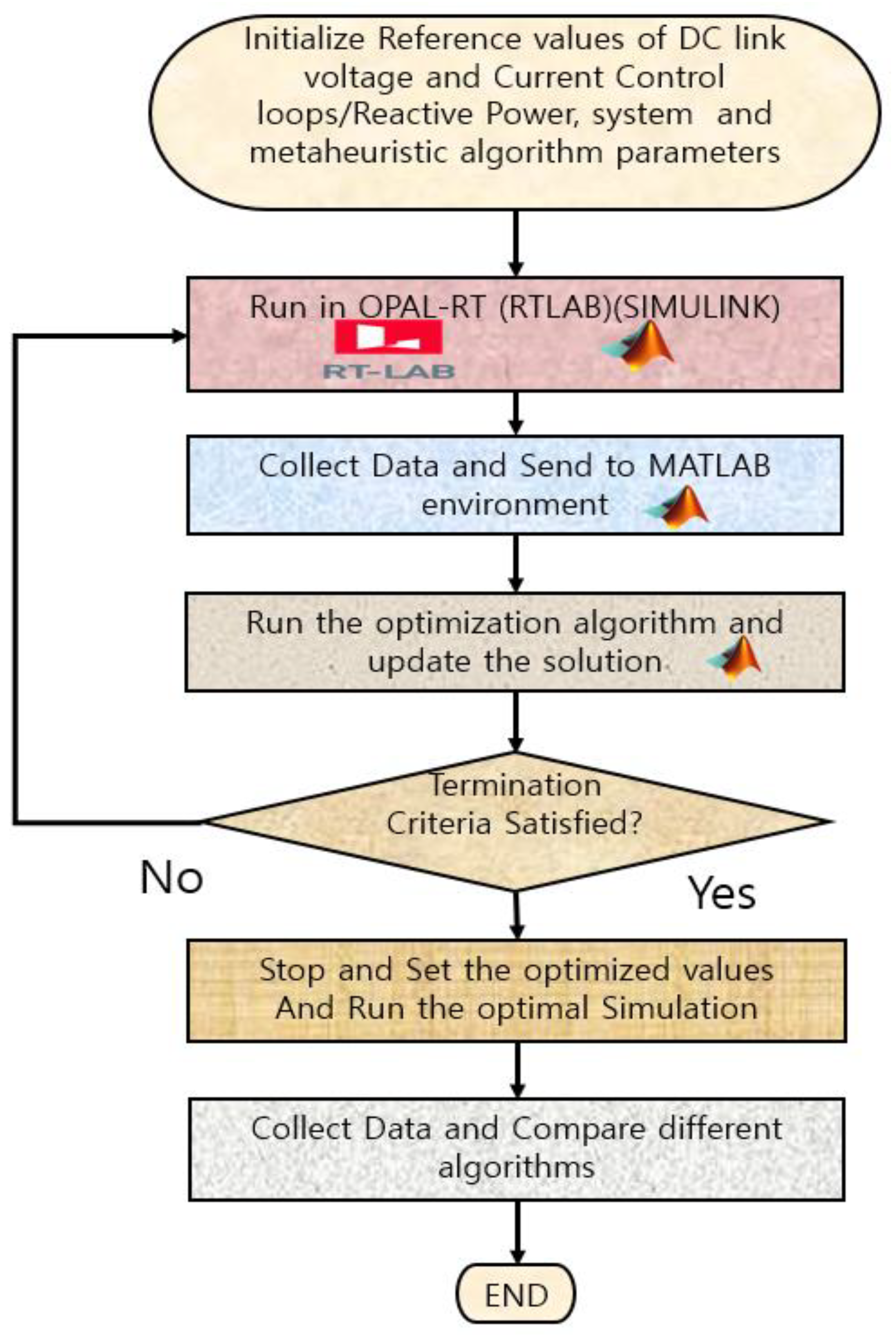
To begin the optimization, the initialization of the system parameters and parameters associated with optimization algorithms must be initiated. Once the initialization is done, the system will be directly simulated in the RTLAB-based Simulink environment, the system responses will be sent to the MATLAB environment, and then optimization algorithms will update the next iteration solutions and feed them into the Simulink environment again. The whole system operates in an iterative manner until the termination criteria or maximum number of generation (iterations) is reached.
Figure 6 describes the operational flowchart for finding the optimal values. The core of the process is the optimization algorithm. In the next section, a brief introduction of three applied optimization algorithms are given.

3.2. Particle Swarm Optimization

Particle swarm optimization (Algorithm 1) [16] is a population-based stochastic optimization technique developed by Eberhart and Kennedy in 1995. The essence of the PSO can be understood by the following equations and the pseudocode:
v g + 1 i = w v g i + c 1 r a n d ( p g i x g i ) + c 1 r a n d ( p g b x g i ) ,
x g + 1 i = x g i + v g + 1 i ,
where x g i and x g + 1 i are particle positions in the g t h and g + 1 t h generations, respectively. v g i and v g + 1 i are particle velocities in g t h and g + 1 t h generations, respectively. w is known as inertia and generally varies within 0 to 1. c 1 and c 2 are known as cognitive and social parameters, respectively, and are generally within the range of 0–2. r a n d is a random number within the range of 0–1. p g i and p g b are best-remembered individual and swarm positions, respectively.
Algorithm 1. PSO
1: Initialize X = Particle/Solution and v = Velocity
2: while gen < max_gen
3:    for each particle x in X do
4:       fx = f(x)
5:          if fx is better than f(xBest)
6:       xBest = x;
7:         end
8:   gBest = best x in X
9:     for each particle x in X do
10:        update velocity and particle position using Equations (11) and (12)
11:    end for
12: end while

3.3. Elephant Herding Optimization

Elephant herding optimization (Algorithm 2) [17] was proposed by Gai-Ge Wang, Suash Deb and Leandro dos S. Coelho in 2015. The algorithm is inspired by the herding behavior of the elephant group. Elephants of different clans live together under the leadership of a matriarch, and male elephants leave the group when they become adults. These two behaviors are modeled into this algorithm, known as clan updating and separating operators. The position of an elephant updates the updating operator. Next, the population diversity is created by separating the operator. The required equations for this optimization given below.
Clan updating operator:
x n e w , c i , j = x c i , j + α ( x b e s t , c i x c i , j ) r ,
where x n e w , c i , j and x c i , j are updated and previous positions of elephant j in clan ci. α [ 0 , 1 ] is a scale factor. x b e s t , c i is the matriarch in the clan. r [ 0 , 1 ] is a uniformly distributed random number.
The fittest elephant in each clan should be updated using Equation (14):
x n e w , c i , j = β x c e n t e r , c i ,
where x c e n t e r , c i , d = 1 n c i j = 1 n c i x c i , j , d and β [ 0 , 1 ] .
Separating Operator:
x w o r s t , c i = x m i n + ( x m a x x m i n + 1 ) r a n d ,
where r a n d [ 0 , 1 ] .
Algorithm 2. EHO
1: Initialize X=Particle/Solution
2: while gen < max_gen
3:  Sort all the elephants according to the fitness
4:  Implement Clan updating operator by Equations (13) and (14)
5:  Implement Separating operator using Equation (15)
6:  Evaluate the population by updated positions
7:  gen = gen + 1;
8: end while

3.4. Plant Propagation Algorithm

The plant propagation algorithm (Algorithm 3) [18] is inspired by propagating plants akin to strawberry plants (Salhi and Fraga, 2011). PPA resembles the way plants, particularly strawberry plants propagate. PPA consists of four simple steps. In step 1, fitness values are normalized using the following equation:
σ [ F ( X j ) ] = F ( X j ) w o r s t B e s t w o r s t ,   j = 1 , 2 , M ,
where j represents the corresponding population. In the next step, few offspring are made to explore the decision space. The number of runners (offspring) created by a solution is proportionate to its normalized fitness value and it is calculated as:
μ j = μ m a x σ j R a n d ,   j = 1 , 2 , M ,
where R a n d [ 0 , 1 ] , and x indicates the ceiling of x.
Next, the distance between the original and the new solutions is calculated as follows:
d i , j = 2 ( 1 σ j ) ( R a n d 0.5 ) j = 1 , 2 , M ,   i = 1 , 2 , N ,
where i is the dimension of the problem.
Then, this distance is used to generate new solutions as follows:
x r , i = x j , i + ( x i U x i L ) d j , i ,
where x i U and x i L are upper and lower bounds of the solution variable, respectively.
Algorithm 3. PPA
1: Initialize X = Particle/Solution
2: while gen < max_gen
3: evaluate the fitness value of solutions
4: for j = 1 to M
5:  evaluate normalized fitness using Equation (16)
6:  evaluate the number of new solutions generated by Equation (17)
7: for i = 1 to N
8:    evaluate the length of the offspring by Equation (18)
9: end for
10: for r = 1 to μ j
11:   for i = 1 to N
12:    evaluate the decision variable ith of new solution rth generated by Equation (19)
13:   end for
14:  end for
15: end for
16: Reform the new population with M best solutions
17: end while
Each of the above algorithms requires an initial value of candidate solutions; an initial velocity is also required for PSO. This can be written as a matrix for ease of computation procedure:
population = [ X 1 X 2 X M ] = [ x 1 , 1 x 1 , 2 x 2 , 1 x 2 , 2 x 1 , N x 2 , N x M , 1 x M , 2 x M , N ] ,
where, X j = jth solution, i = population size, and N = problem dimension.

4. Experimental Setup and Simulation Results

The experiment was set up with the data given in Table 1. For the machine-In-loop experiment, the help of OPAL-RT (OP5600) real-time digital simulator was taken. The model was built in RTLAB using Simulink-based toolbox, and optimization source-codes were written in MATLAB script. The experimental setup is shown in Figure 7.
For a global solution, a closed search space is required, or in other words, the solutions must be bounded within where the optimal value can be tracked. Mathematically,
x m i n x x m a x .
However, in some systems if the search space boundary is unknown then it is difficult to find an initial value for starting the optimization. Hence, before conducting the actual optimization process, we randomly ran the simulation 30 times with a random data range to find a valid search space within where we can find the optimal solution. After such trials, the following range was found for each of the parameters given in Table 2.
In every metaheuristic algorithm, it is required to deal with some parameters to control the convergence speed of the algorithm. These parameters are generally user-defined parameters, which means the user can set those parameters and examine for which set of values optimal results are achieved. For example, for PPA algorithm the only such parameter is μ m a x , which controls the number of runners created by a solution. If this number increases, a solution will create more runners, but simulation time will increase. Hence it should be chosen in such a way that optimal result is found under minimum possible simulation time. For the considered algorithms, the parameters and their values are given in Table 3.
Also, the population number and number of generation were taken as 20 and 30, respectively.
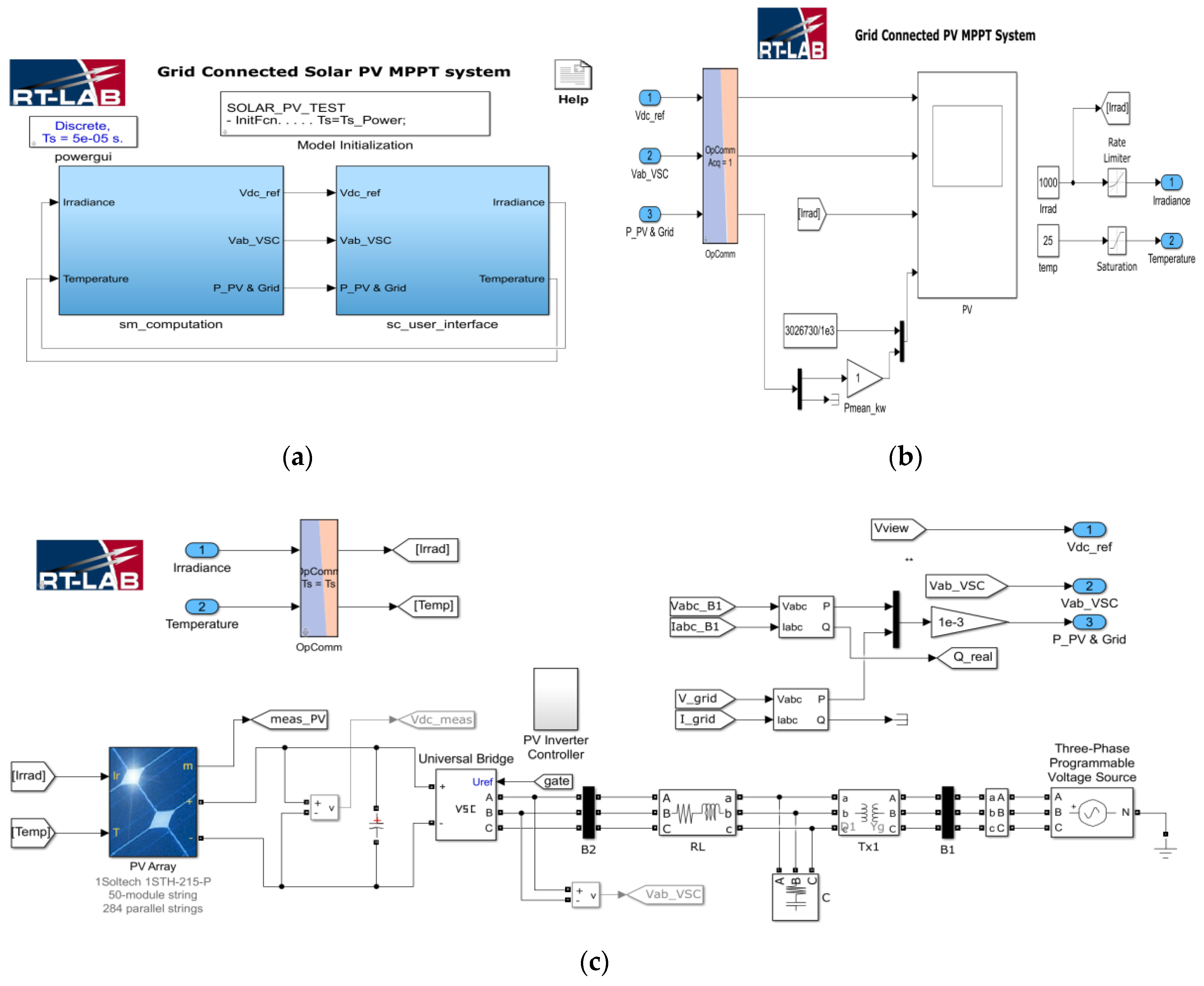
In Figure 8, the simulation figure in the RT-LAB environment has been shown. Unlike Simulink environment, RTLAB-based simulator requires two different blocks for real-time operation. The first block is sm_computation block, where the main system and corresponding controllers were developed. In the second block, sc_user_interface, the input for the system and data visualization blocks are drawn. Fractional order PI controller has been implemented using FOMCON toolbox. The inputs of the system were the solar irradiance and temperature.
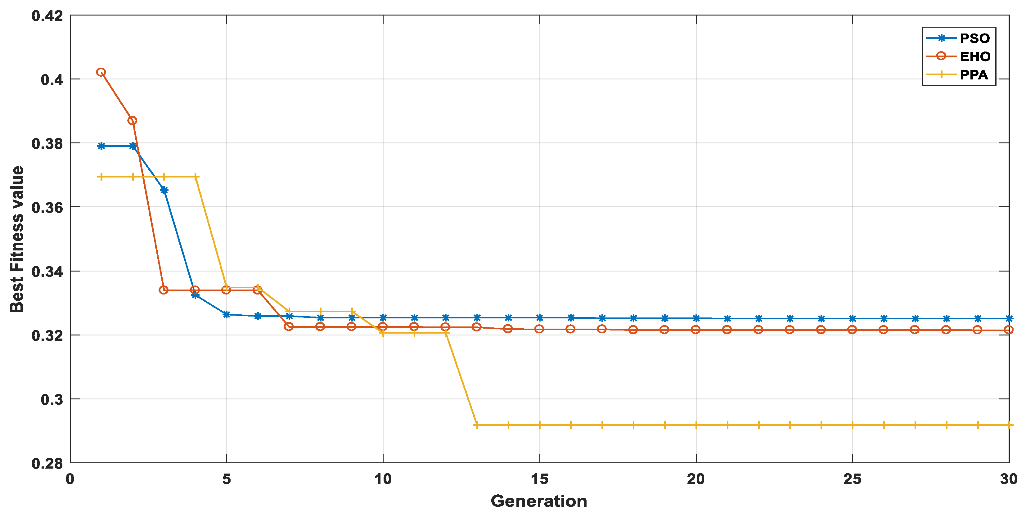
After the completion of the simulation, the best fitness value can be obtained from Figure 9 and it can be understood that PPA outperforms EHO- and PSO-based controllers. For PSO, conventional PI controller was used; for EHO and PPA, FOPI was used. The reason behind the better solution from PPA is due to the creation of multiple runners from each solution (Equation (17)) and storing only the best population in each generation. In this problem we have chosen maximum value of μ m a x as No. of population/5, i.e., 20/5 = 4.
Hence each of the solutions can generate a maximum of four different solutions from its original solution. As a result, in each generation, the total number for population can vary from 20–80. But to maintain uniformity, after completion of each generation only the 20 best populations are chosen from the 20–80 populations. The process repeats in each iteration.
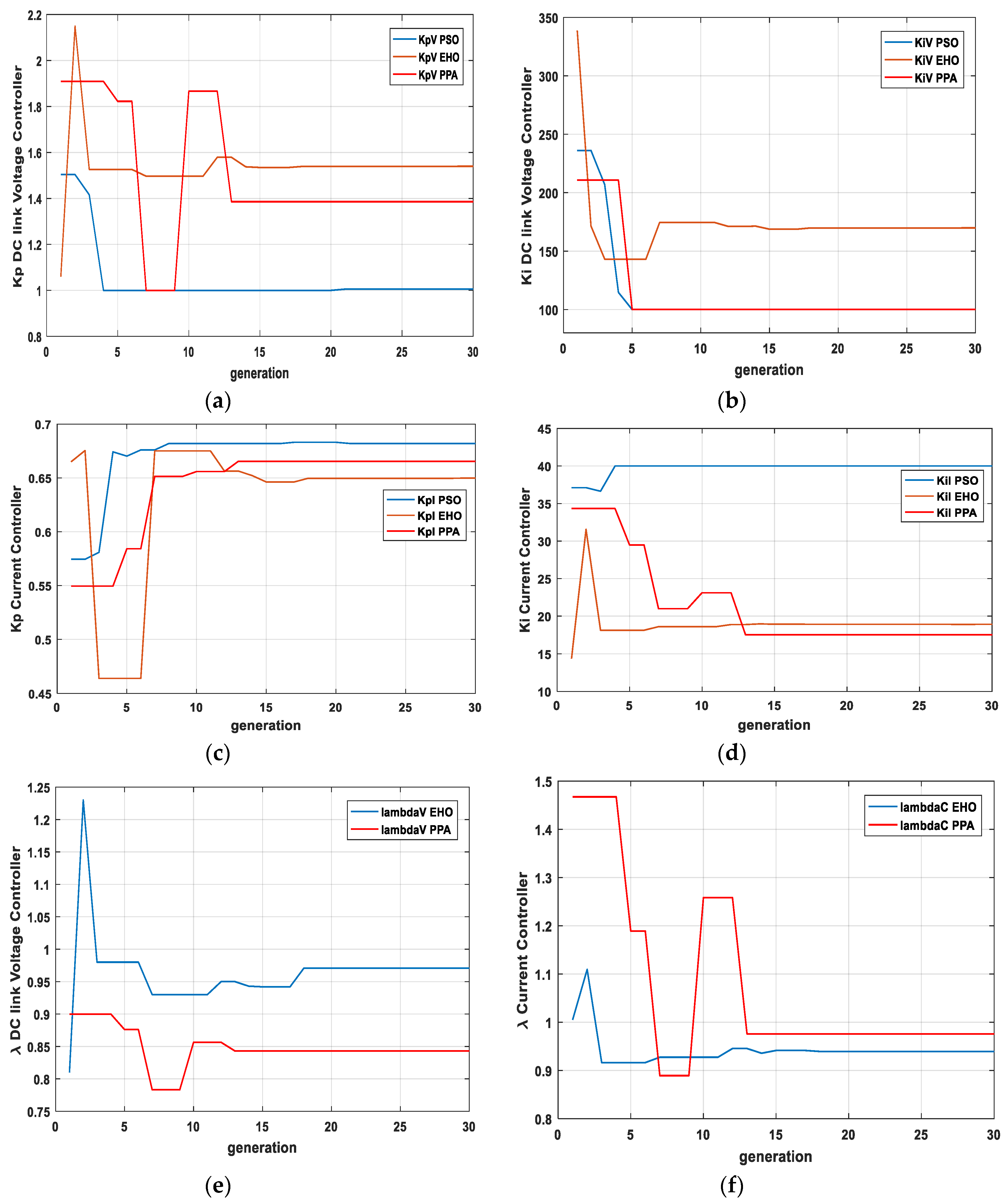
Figure 10 shows the gain parameter trajectory over time. For PSO Kp (DC link voltage controller) gain value changes until the 21st generation, But Ki (DC link voltage controller) gain reaches the minimum value of the range at the fifth generation and could not improve further. Kp (current control loop) for PSO finally stops changing at iteration 21, whereas Ki (current control loop) reaches the maximum value at the fourth generation.
For EHO, there is no such incident of reaching the maximum or minimum values without further improvement.
In the case of PPA, there is only such a case (Ki (DC link voltage controller)) where it reaches the minimum value and could not improve further. However, due to the increase of the degree of freedom in control action with the help of λ parameter, it still improves the overall response and hence reduces the error.
Table 4 represents the optimal values of the controller parameters, in other words, the final values of the gain parameters from the trajectory plot of Figure 10.
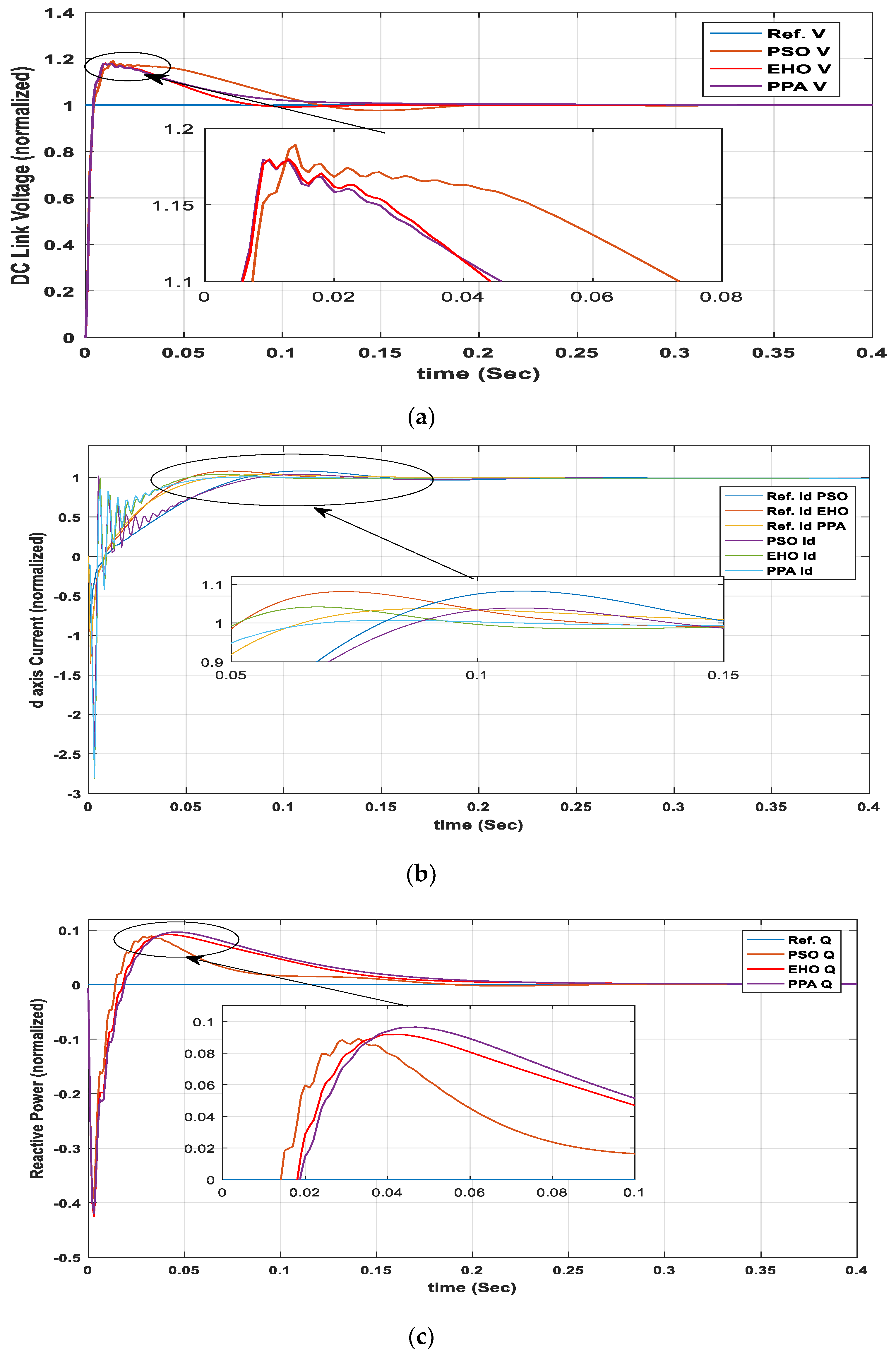
The optimal response of the DC link voltage controller, d-axis current and reactive power/q-axis current control loop is given in Figure 11. Optimization was done under the maximum irradiance of 1000 w/m2 and a fixed temperature of 25 °C. In Figure 11b, unlike Figure 11a,c, there are different individual reference values for each of the optimization algorithms. This is because the reference value for the d-axis current controller comes from the output of the DC link voltage controller. As responses from different optimization techniques provide different outputs from the DC link voltage controller, the reference value also changes for the d-axis current controller.
The settling time was calculated by finding the response when it comes to the ± 2 % band of the desired response. The peak overshoot was calculated using:
%   Peak   Overshoot = P e a k   v a l u e f i n a l   v a l u e f i n a l   v a l u e × 100 .
As the reference value for the reactive power controller is 0 (unity power factor condition), hence the percent peak overshoot for this term was calculated using a modified equation as follows:
%   Peak   Overshoot = P e a k   v a l u e f i n a l   v a l u e f i n a l   v a l u e + ε × 100 .
The value of ε is an arbitrary small number, which should be the same, irrespective of the algorithm to maintain uniformity. The time responses of Figure 11, the objective function, and convergence speed are listed in Table 5.
From Table 5, in terms of objective function, PPA shows a better result over PSO and EHO. However, at the molecular level (settling time and peak overshoot) the performance can be varied. For example, settling time for DC link voltage controller and Iq/Q controller in terms of PPA is greater than PSO and EHO. Also, peak overshoot of Iq/Q for PPA-based controller is greater than PSO- and EHO-based controllers. Hence, it is difficult to say that PPA is better than EHO and PSO from the tabular analysis only. So, a spider graph-based [19] approach is proposed to compare the indexes to find out the best algorithm.

4.1. Index Comparison

For index-based performance analysis, we have considered eight indexes where three are for settling time, three are for peak overshoot, one is for the objective function, and the remaining is for converge speed of the optimization algorithms. As the indexes have different ranges, we have normalized them using their maximum values and plotted them in the spider graph to compare the indexes. The normalized index value is calculated using the following equation:
Index   Value = A c t u a l   I n d e x   V a l u e C o r r e s p o n d i n g   I n d e x   M a x i m u m   V a l u e   a c c r o s s   t h e   A l g o r i t h m s .
From the above equation, it can be understood that any value which is closer to 1 represents the maximum value. As this is a minimization problem, the lesser the value is, the better the index is. Hence, the smaller boundary inside the solid line represents the better solution.
Also, from Figure 12, it can be easily seen that although for some indexes PPA reaches the maximum value, extremely smaller values in other indexes makes the inner area smaller compared to other algorithms. So, it can be said that PPA outperforms PSO and EHO in this problem.

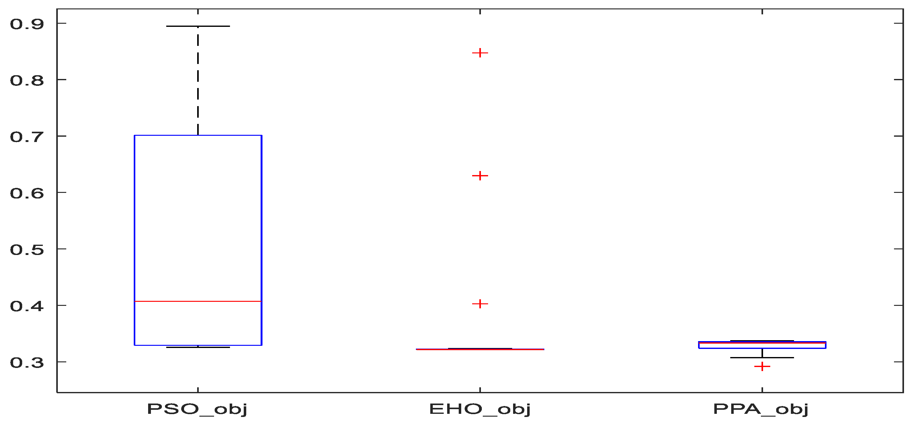
4.2. Boxplot Analysis for Global Optimization Analysis

The boxplot in Figure 13. represents the fitness function values corresponding to the population at the final iteration (generation). The fitness functions for EHO and PPA are distributed over a narrow range, except for a few far points (red + markers) for EHO. Also, the means for PPA and EHO are much less than for PSO. The lowest value of the objective function is found using the PPA-based algorithm which validates the result from Figure 9. The smaller range of objective function signifies that all the population has reached the global optimal solution.

5. Plant Propagation Algorithm-Based Controller Performance Analysis

5.1. Power Quality Analysis Through Total Harmonic Distortion (THD) Analysis

For smoother operation, the current injected by the inverter should not possess harmonics and THD should be less than 5% according to IEEE standards 929–2000 [20]. Using the proposed controllers, from Figure 14 the THD found was only 1.15% which is much less than maximum allowable value.

5.2. Performance under Varied Conditions

During the optimization process, the controller was tuned under only a certain condition, but to be a successful controller it must run optimally irrespective of the environmental (irradiance and temperature) conditions. Hence the controller was tested under varied irradiance conditions. A properly tuned controller should be able to deliver real and reactive power as per the reference values. For the testing purpose, the irradiance of the system varied quickly with a wide range of values. It started with 200 W/m2, then suddenly changed to 800 W/m2 at 3 s, followed by 600, 700, and 400 W/m2 at 4, 5, and 6 s respectively. The temperature was fixed at 25 °C, although it can also be varied. The corresponding reference and simulated power outputs can be seen in Figure 15c. Reference reactive power was also varied during this period in such a way that it does not violate the Q S 2 P 2 condition. The DC link voltage controller was found to track the reference value very efficiently.
The performance of the proposed controllers was also tested under voltage sag condition. With a symmetrical voltage sag of 50% with 0.15 s duration, the controllers were still able to reach the steady-state comfortably. The sudden rises in responses at 0.2 and 0.35 s from Figure 16b,c represent the changes in voltage level.
In Figure 15 and Figure 16, red lines belong to references and blue lines belongs to response values.
To validate the robustness of the PPA-based proposed controller, performance under varied conditions of the system parameters such as filter and transformer resistances and inductances were also conducted. Parameters are varied between −10% to 10% of their nominal values, which can be found in Table 1. The corresponding fitness values are given in Table 6.
From Table 6 it can be seen that although system parameters varied widely between −10% to +10%, the objective function values did not vary much and stayed very near to the tested condition objective function value (0.2918).

6. Conclusions and Future Work

In this work, we have developed PPA- and EHO-based fractional order PI controllers which outperform the PSO-based conventional PI controller for grid-connected three-phase single-stage solar PV systems. The controllers were optimized and tested using a real-time digital simulator (OPAL-RT) by the machine-in-loop approach. The best algorithm was chosen not only based on objective function but with other performance indexes also. The performance indexes have been compared over eight categories with help of spider graphs. Also, convergence to the optimal solution by means of objective functions over the population at the final generation was presented by the boxplot analysis. After all these rigorous processes of analysis, the PPA-based controller was chosen as the best controller over the other two algorithms. The chosen controller performance under varied irradiance, system parameters, and voltage sag is also tested and found to be very efficient with a lower value of THD of inverter-injected current.
This work is a part of the development of Platform Design and Application Technologies for Alphagrid under Korea Electric Power Corporation. The work will be extended to estimate/match the other parameters present in the system with respect to the actual values using the considered metaheuristic algorithms to develop a 1:1 matching digital twin. The developed approach in this work can be effectively applied to system parameter tuning so that the responses from real and cyber systems match each other in real time.

Author Contributions

M.A.Z. devised the idea, completed the simulations and prepared the manuscript. D.W. has supervised and commented on the manuscript. All the authors read and approved the final manuscript.

Acknowledgments

This work was supported by INHA UNIVERSITY Research Grant (59309-01).

Conflicts of Interest

The authors declare no conflict of interest.

References

  1. Jumani, T.A.; Mustafa, M.W.; Rasid, M.M.; Mirjat, N.H.; Baloch, M.H.; Salisu, S. Optimal Power Flow Controller for Grid-Connected Microgrids using Grasshopper Optimization Algorithm. Electronics 2019, 8, 111. [Google Scholar] [CrossRef]
  2. Sharifian, M.B.; Mohamadrezapour, Y.; Torabzade, S.; Hosseinpour, M. Single-Stage Grid Connected Photovoltaic System with Reactive Power Control and Adaptive Predictive Current Controller. J. Appl. Sci. 2009, 9, 1503–1509. [Google Scholar] [CrossRef]
  3. Tafti, H.D.; Maswood, A.I.; Ukil, A.; Gabriel, O.H.P.; Ziyou, L. NPC Photovoltaic Grid-Connected Inverter using Proportional-Resonant Controller. In Proceedings of the 2014 IEEE PES Asia-Pacific Power and Energy Engineering Conference (APPEEC), Hong Kong, China, 7–10 December 2014. [Google Scholar] [CrossRef]
  4. Tripathi, R.N.; Hanamoto, T. FRIT Based Optimized PI Tuning for DC Link Voltage Control of Grid Connected Solar PV. In Proceedings of the IECON 2015-41st Annual Conference of the IEEE Industrial Electronics Society, Yokohama, Japan, 9–12 November 2015. [Google Scholar] [CrossRef]
  5. Anjaneyulu, Y.A.; Khobragade, J. Single Phase Single Stage Grid Connected PV System with Improved Power Quality. In Proceedings of the 2016 International Conference on Automatic Control and Dynamic Optimization Techniques (ICACDOT), Pune, India, 9–10 September 2016. [Google Scholar] [CrossRef]
  6. Touil, S.-A.; Boudjerda, N.; Boubakir, A.; Boudouda, A. Sliding Mode Control of a Grid-Connected Photovoltaic Source via a Three-Phase Inverter using Incremental Conductance MPPT. In Proceedings of the 5th International Conference on Electrical Engineering–Boumerdes (ICEE-B), Boumerdes, Algeria, 29–31 October 2017. [Google Scholar] [CrossRef]
  7. Azghandi, M.A.; Barakati, M.; Wu, B. Dynamic Modeling and Control of Grid-Connected Photovoltaic Systems based on Amplitude-Phase Transformation. Iran. J. Electr. Electron. Eng. 2018, 4, 342–352. [Google Scholar] [CrossRef]
  8. Mohamed, S.R.; Jeyanthy, P.A.; Devaraj, D.; Shwehdi, M.H.; Aldalbahi, A. DC-Link Voltage Control of a Grid-Connected Solar Photovoltaic System for Fault Ride-Through Capability Enhancement. Appl. Sci. 2019, 9, 952. [Google Scholar] [CrossRef]
  9. Khawla, E.M.; Chariag, D.E.; Sbita, L.A. Control Strategy for a Three-Phase Grid Connected PV System under Grid Faults. Electronics 2019, 8, 906. [Google Scholar] [CrossRef]
  10. Islam, S.U.; Zeb, K.; Din, W.U.; Khan, I.; Ishfaq, M.; Busarello, T.D.C.; Kim, H.J. Design of a Proportional Resonant Controller with Resonant Harmonic Compensator and Fault Ride. Trough Strategies for a Grid-Connected Photovoltaic System. Electronics 2018, 7, 451. [Google Scholar] [CrossRef]
  11. MathWorks. Available online: https://www.mathworks.com/help/physmod/sps/powersys/ref/pvarray.html (accessed on 5 August 2019).
  12. Kamran, M.; Mudassar, M.; Fazal, M.R.; Asghar, M.U.; Bilal, M.; Asghar, R. Implementation of improved Perturb & Observe MPPT technique with confined search space for standalone photovoltaic system. J. King Saud Univ.-Eng. Sci. 2018. [Google Scholar] [CrossRef]
  13. Wu, B.; Lang, Y.; Zargari, N.; Kouro, S. Power Conversion and Control of Wind Energy Systems; Wiley: Hoboken, NJ, USA, 2011; pp. 52–148. [Google Scholar]
  14. Ameer, L.; Saleh, A.; Obed, A. Speed Control of Brushless DC Motor based on Fractional Order PID Controller. Int. J. Comput. Appl. 2014, 95, 1–6. [Google Scholar] [CrossRef]
  15. Tan, W.; Liu, J.; Chen, T.; Marquez, H.J. Comparison of some well-known PID tuning formulas. Comput. Chem. Eng. 2006, 30, 1416–1423. [Google Scholar] [CrossRef]
  16. Kennedy, J.; Eberhart, R. Particle Swarm Optimization. In Proceedings of the ICNN’95-International Conference on Neural Networks, Perth, WA, Australia, 27 November–1 December 1995. [Google Scholar] [CrossRef]
  17. Wang, G.-G.; Deb, S.; Coelho, L. Elephant Herding Optimization. In Proceedings of the 2015 3rd International Symposium on Computational and Business Intelligence (ISCBI), Bali, Indonesia, 7–9 December 2015. [Google Scholar] [CrossRef]
  18. Bozorg-Haddad, O.; Solgi, M.; Loaciga, H.A. Meta-Heuristic and Evolutionary Algorithms for Engineering Optimization; Wiley: Hoboken, NJ, USA, 2017. [Google Scholar]
  19. FusionCharts. Available online: https://www.fusioncharts.com/resources/chart-primers/radar-chart (accessed on 1 October 2019).
  20. IEEE. IEEE Recommended Practice for Utility Interface of Photovoltaic (PV) Systems; IEEE: Piscataway, NJ, USA, 2000. [Google Scholar]
Figure 1. Single-stage three-phase grid-connected photovoltaic (PV) system: (a) overall system; (b) inside inverter control block.
Applsci 09 04269 g001
Figure 2. Equivalent circuit of PV cell; I–V and P–V characteristics curves.
Applsci 09 04269 g002
Figure 3. Perturbation and observation-based maximum power point tracking (MPPT).
Applsci 09 04269 g003
Figure 4. Outer voltage and inner current control loops.
Applsci 09 04269 g004
Figure 5. Fractional order PI controller: (a) block diagram; (b) graphical representation.
Applsci 09 04269 g005
Figure 6. Flowchart of the optimal value finding.
Applsci 09 04269 g006
Figure 7. Experimental setup.
Applsci 09 04269 g007
Figure 8. Simulink model for real-time machine-in-loop (MIL) simulation in OPAL-RT: (a) RTLAB-based Simulink interface; (b) sc_user_interface block; (c) sm_computation block.
Applsci 09 04269 g008
Figure 9. Fitness value.
Applsci 09 04269 g009
Figure 10. Gain parameters’ trajectory with respect to generation: (a) Kp gain of DC link voltage controller; (b) Ki gain of DC link voltage controller; (c) Kp gain of d- and q-axis current controller; (d) Ki gain of d- and q-axis current controller; (e) λ of DC link voltage controller; (f) λ of current controller.
Applsci 09 04269 g010
Figure 11. Controller time response. (a) DC link voltage controller; (b) d-axis current controller; (c) q-axis current/reactive power controller.
Applsci 09 04269 g011
Figure 12. Eight-axis spider graph for index comparison among the algorithms.
Applsci 09 04269 g012
Figure 13. Box plot for the objective function of the final generation population for every optimization technique.
Applsci 09 04269 g013
Figure 14. Total harmonic distribution (THD) analysis of inverter-injected current
Applsci 09 04269 g014
Figure 15. Performance of the proposed controller under different irradiance conditions.
Applsci 09 04269 g015
Figure 16. Controller performance under symmetrical 50% voltage sag.
Applsci 09 04269 g016
Table 1. System parameters.
ParametersValuesParametersValues
Plant Capacity 3026 kVAFilter Resistance0.0015 pu
Grid Voltage 4.16 kV ( V L L , r m s ) Filter Inductance0.15 pu
Frequency 60 HzFilter Capacitance0.1 pu
DC Link Capacitance0.0720 FTransformer Resistance0.0012 pu
DC Link Voltage 1450 VdcTransformer Inductance0.03 pu
Each Unit Capacity 213.15 WSwitching Frequency1980 Hz
No. of Series Units50Sampling Time50 µs
No. of Parallel Units213
Table 2. Search space boundary values for gain parameters.
Parameter K p v K i v λ v K p I K i I λ I
Max value0.8401.544001.5
Min value0.2100.7511000.75
K p v ,   K i v , and λ v are parameters related to the outer voltage control loop, and K p I ,   K i I , and λ I are related to inner current control loop.
Table 3. Parameters for different metaheuristic algorithms.
AlgorithmParameterValues
PSO C 1 , C 2 , w 1.5, 1.5, 0.9
EHO α ,   β 0.5, 0.5
PPA μ m a x Population number/5
Table 4. Optimal value of gain parameters.
ControllerDC Link Voltage ControllerCurrent Controller
ParameterKpKi λ KpKi λ
PSO1.0054100-0.682040-
EHO1.5398169.85230.97070.649818.90240.9394
PPA1.38581000.84310.665417.50340.9757
Table 5. Objective function, time responses and convergence speed of different algorithms.
IndexPSOEHOPPA
Objective Function0.3250940.3214710.2918
DC link controller Settling time (sec)0.12500.09000.1270
Id controller settling time (sec)0.14900.10600.0720
Iq/Q controller settling time (sec)0.10300.15500.1670
DC link controller Peak Overshoot (%)18.917817.991217.9831
Id controller peak overshoot (%)4.73175.04021.580398
Iq/Q Controller peak overshoot (%)89.105691.919196.4454
Convergence Speed (iteration)211813
Table 6. Fitness values under varied parameter values.
Parameters R g and L g
% Changes of the Nominal Values−10%−5%+5%+10%
Objective function values0.30460.29690.28500.3121

