Comparing AutoDock and Vina in Ligand/Decoy Discrimination for Virtual Screening

Abstract

AutoDock and Vina are two of the most widely used protein–ligand docking programs. The fact that these programs are free and available under an open source license, also makes them a very popular first choice for many users and a common starting point for many virtual screening campaigns, particularly in academia. Here, we evaluated the performance of AutoDock and Vina against an unbiased dataset containing 102 protein targets, 22,432 active compounds and 1,380,513 decoy molecules. In general, the results showed that the overall performance of Vina and AutoDock was comparable in discriminating between actives and decoys. However, the results varied significantly with the type of target. AutoDock was better in discriminating ligands and decoys in more hydrophobic, poorly polar and poorly charged pockets, while Vina tended to give better results for polar and charged binding pockets. For the type of ligand, the tendency was the same for both Vina and AutoDock. Bigger and more flexible ligands still presented a bigger challenge for these docking programs. A set of guidelines was formulated, based on the strengths and weaknesses of both docking program and their limits of validation.

1. Introduction

The use of computational methods is a crucial part of the drug discovery, development, and optimization process. Protein–ligand docking and virtual screening are two of the most used techniques in this field that continue to show promise in hit identification and subsequent optimization [1]. They are also helpful tools for drug repositioning [2,3,4]. These methods are effective and fast, and allow researchers to evaluate large virtual databases of molecular compounds as a first attempt to guide the selection of more limited sets of compounds for experimental testing. They do, however, possess few limitations [5,6].

Protein–ligand docking is a computational technique that predicts the conformation and orientation (pose) of a ligand when it is bound to a given protein [1,7,8,9,10,11,12]. With this method, the ligand-target interactions are modeled to achieve an optimal complementarity of steric and physicochemical properties [13]. This methodology has made possible the visualization of the potential interactions between a ligand and its target [14].

Docking, however, still faces difficulties, particularly regarding the correct modeling of ligand and protein flexibility [15,16,17,18] and of water-mediated interactions [18,19]. It is widely used for small molecules, but its use for small peptides and other larger biomolecules has only been under development in the last decade [20,21,22].

Typically, the docking software is an interplay between the search algorithm, which explores and generates different poses of the ligand, and the scoring function, which estimates the binding affinities of the poses previously created, discriminating between the best and not so good alternatives [1,5]. This estimate, which in some cases is a prediction of the free energy of binding, must be able to discriminate between molecules that bind to the target and those that do not [23]. When looking at the two enantiomers, for example, it is still not possible to identify the most active form with most of the scoring functions used by the most common docking software [24].

Even with all the significant improvements in computational power and docking software, considering all interactions that happen when a ligand binds to its target is an extremely challenging task. In order to be rigorous, the scoring functions would have to be much more complex, involve quantum calculations and, thus, these assays would turn out to be considerably expensive and time-consuming. When applying a virtual screening protocol, one wishes to screen very large databases of compounds in a relatively small period of time and, therefore, scoring functions are often simplified to improve the speed and cost of the computational screenings [6]. These simplifications come with a cost in accuracy, which might not be problematic for one ligand-target situation but takes a much more challenging scope when talking about virtual screening of thousands or millions of compounds [5].

The goal of virtual screening (VS) is to guide the selection of molecules for experimental testing. In these assays, millions of compounds are docked into one specific target and only a selection of the top scores proceeds for experimental testing. If a scoring functions fails to identify a potential strong binder, then, it remains hidden among those million compounds, despite their pharmacological potential. In fact, that is one of the main problems in VS, the false negatives, or molecules that the docking fails to identify as strong ligands. False positives are also a problem, that is, molecules that are incorrectly identified as strong binders. These molecules, however, are easily discarded in the preliminary experimental assays [25].

It is, however, difficult to compare the performance of different docking alternatives because each software handles the target and ligand in different manners. Additionally, it has been shown that the docking and VS results vary according to the type of target and ligand molecule [26,27,28,29,30]. In this study, two of the most commonly used docking tools—AutoDock (version 4.2.6) and Vina (AutoDock Vina)—were evaluated for different types of targets and ligands, using an unbiased reference validation set—Directory of Useful Decoys–Enhanced (DUD–E) [31]. Both docking programs are widely used to this day, for a large diversity of targets and problems [32,33,34,35,36,37,38,39].

AutoDock 4 is a well-known docking program developed by Morris and co-workers [40,41,42,43] at the Scripps Research Institute. Its free availability to academic users, together with the good accuracy and high versatility shown, had made it a very popular first choice for new users and have contributed to a widespread use of AutoDock, well portrayed in its impressively high number of citations. AutoDock 4 offers a variety of search algorithms and a scoring function that is based on a linear regression analysis, the Assisted Model Building with Energy Refinement (AMBER) force field, and a large set of diverse protein–ligand complexes with known inhibition constants. The program could be used with a visual interface called AutoDock Tools (ADT) which ensures an efficient analysis of the docking results.

AutoDock Vina [44,45,46] is a docking program developed by Trott and Olson also at the Scripps Research Institute, La Jolla, California, following the success of previous AutoDock versions. Vina is freely accessible to a large number of users, as it is open source. AutoDock Vina inherits some of the ideas and approaches of AutoDock 4, but it is designed in a conceptually different way. It offers significant improvements in the average accuracy of the binding mode predictions, while also being up to two orders of magnitude faster than AutoDock 4. It also features new search algorithm and a hybrid scoring function, combining empirical and knowledge-based scoring function. Its multi-core capability, high performance and enhanced accuracy, ease-of-use and free availability have contributed to an extremely fast dissemination through the docking community, well-portrayed in the high number of citations of the original paper. Its high computational efficiency and ability to use multiple CPUs or CPU cores also makes this program a competitive alternative for virtual screening.

The Directory of Useful Decoys–Enhanced (DUD–E) [31] holds a collection of decoys and ligands for benchmarking virtual screening, containing 22,432 active compounds and their affinities against 102 targets set by Huang et al. For each of the active compounds (i.e., the ligands), this database contains a set of 50 “decoys”, i.e., molecules with similar 1-D physico-chemical properties to remove bias (e.g., molecular weight, calculated LogP), but dissimilar 2-D topology to be likely non-binders, i.e., inactives. These characteristics make DUD–E a challenging dataset to test scoring functions and protein–ligand docking algorithms. Ideally, the perfect scoring function would rank the active molecules higher than the decoys, but that is not often the case.

2. Materials and Methods

The performance of AutoDock 4 and Vina was measured using the Directory of Useful Decoys–Enhanced (DUD–E). DUD–E contains a large collection of decoys and ligands that can be used for benchmarking ligand/decoys discrimination in virtual screening tests. The DUD–E dataset has been widely used to validate data from other open source such as Dock [47,48] and commercial programs such as Gold, Glide, Surflex, and FlexX [48]. It is also frequently used to validate the development of new consensus scoring functions [38,49,50,51,52,53,54].

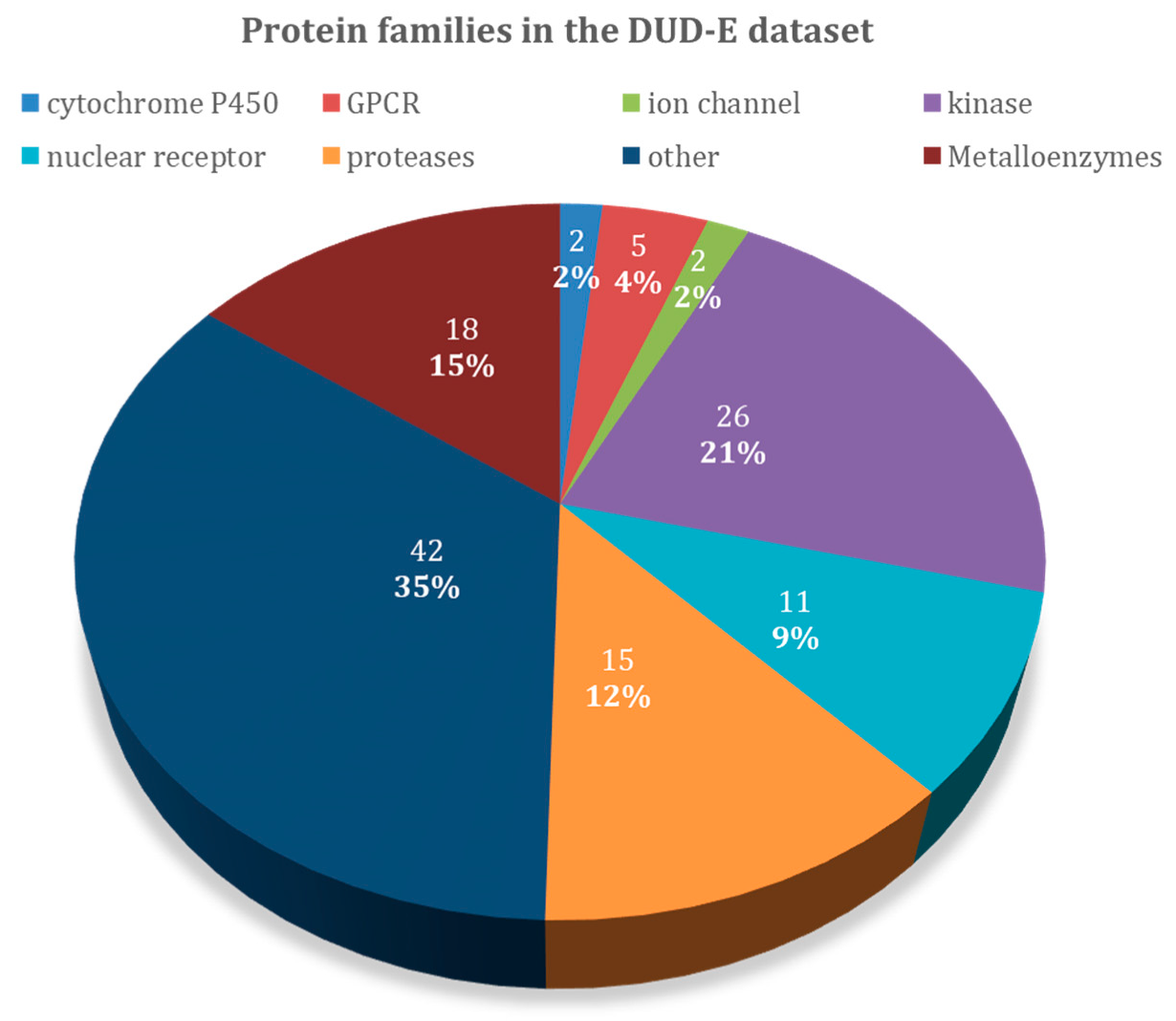
An overview of the 102 protein-targets in DUD–E can be found in Figure 1, and

Table 1. Protein targets evaluated in this study as part of DUD–E with indication of the different classes of targets considered.

Target Class	DUD–E Code	PDB Code	Protein Name	Ligands	Decoys	Metal
cytochrome P450	CP2C9	1R9O	Cytochrome P450 2C9	120	7446
	CP3A4	3NXU	Cytochrome P450 3A4	170	11,796
G protein-coupled receptor	AA2AR	3EML	Adenosine A2a receptor	482	31,498
	ADRB1	2VT4	Beta-1 adrenergic receptor	247	15,843
	ADRB2	3NY8	Beta-2 adrenergic receptor	231	14,994
	CXCR4	3ODU	C-X-C chemokine receptor type 4	40	3406
	DRD3	3PBL	Dopamine D3 receptor	480	34,022
Ion channel	GRIA2	3KGC	glutamate receptor ionotropic AMPA2	158	11,832
	GRIK1	1VSO	glutamate receptor ionotropic kainate 1	101	6547
Kinases	ABL1	2HZI	Tyrosine-protein kinase ABL	182	10,750
	AKT1	3CQW	Serine/threonine-protein kinase AKT	293	16,426	Mn2+
	AKT2	3D0E	Serine/threonine-protein kinase AKT2	117	6893
	BRAF	3D4Q	Serine/threonine-protein kinase B-raf	152	9942
	CDK2	1H00	Cyclin-dependent kinase 2	474	27,830
	CSF1R	3KRJ	Macrophage colony stimulating factor receptor	166	12,144
	EGFR	2RGP	Epidermal growth factor receptor erbB1	545	35,020
	FAK1	3BZ3	Focal adhesion kinase 1	100	5350
	IGF1R	2OJ9	Insulin-like growth factor I receptor	148	9291
	JAK2	3LPB	Tyrosine-protein kinase JAK2	107	6495
	KIT	3G0E	Stem cell growth factor receptor	166	10,447
	KITH	2B8T	Thymidine kinase	57	2850
	KPCB	2I0E	Protein kinase C beta	135	8692
	LCK	2OF2	Tyrosine-protein kinase LCK	420	27,374
	MAPK2	3M2W	MAP kinase-activated protein kinase 2	101	6147
	MET	3LQ8	Hepatocyte growth factor receptor	166	11,240
	MK01	2OJG	MAP kinase ERK2	79	4548
	MK10	2ZDT	c-Jun N-terminal kinase 3	104	6599
	MK14	2QD9	MAP kinase p38 alpha	578	35,810
	MP2K1	3EQH	Dual specificity mitogen-activated protein kinase 1	121	8147	Mg2+
	PLK1	2OWB	Serine/threonine-protein kinase	107	6797	Zn2+
	ROCK1	2ETR	Rho-associated protein kinase 1	100	6297
	SRC	3EL8	tyrosine-protein kinase SRC	524	34,454
	TGFR1	3HMM	TGF-beta receptor type I	133	8498
	VGFR2	2P2I	Vascular endothelial growth factor receptor 2	409	24,927
	WEE1	3BIZ	Serine/threonine-protein kinase	102	6148
Nuclear receptor	ANDR	2AM9	Androgen Receptor	269	14,344
	ESR1	1SJ0	Estrogen receptor alpha	383	20,663
	ESR2	2FSZ	Estrogen receptor beta	367	20,182
	GCR	3BQD	glucocorticoid receptor	258	14,987
	MCR	2AA2	Mineralocorticoid receptor	94	5146
	PPARA	2P54	Peroxisome proliferator-activated receptor alpha	373	19,356
	PPARD	2ZNP	Peroxisome proliferator-activated receptor delta	240	12,223
	PPARG	2GTK	Peroxisome proliferator-activated receptor gamma	484	25,256
	PRGR	3KBA	Progesterone receptor	293	15,642
	RXRA	1MV9	retinoid X receptor alpha	131	6935
	THB	1Q4X	Thyroid hormone receptor beta-I	103	7441
Proteases	ACE	3BKL	Angiotensin-converting enzyme	282	16,864	Zn2+
	ADA17	2OI0	protease	532	35,809	Zn2+
	BACE1	3L5D	Beta-secretase 1	283	18,082
	CASP3	2CNK	Caspase-3	199	10,692
	DPP4	2I78	Dipeptidyl peptidase IV	533	40,916
	FA10	3Kl6	Coagulation factor X	537	20,023
	FA7	1W7X	Coagulation factor VII	114	6245
	HIVPR	1XL2	human immunodeficiency virus type 1 protease	536	35,688
	LKHA4	3CHP	Leukotriene A4 hydrolase	171	9448	Zn2+
	MMP13	830C	Matrix metalloproteinase 13	572	37,126	Zn2+
	RENI	3G6Z	Renin	104	6956
	THRB	1YPE	Thrombin	461	26,948
	TRY1	2AYW	Trypsin I	449	25,914
	TRYB1	2ZEC	Tryptase beta-I	148	7643
	UROK	1SQT	Urokinase-type plasminogen activator	162	9841
Miscellaneous	AMPC	1L2S	Beta-lactamase	48	2832
	HIVRT	3NF7	human immunodeficiency virus type 1 integrase	100	6644
	KIF11	3CJO	Kinesin-like protein 1	116	6848	Mg2+
Other	ACES	1_e66	Acetylcholinesterase	453	26,234
	ADA	2E1W	Adenosine deaminase	93	5449	Zn2+
	ALDR	2HV5	Aldose reductase	159	8995
	AOFB	1S3B	Monoamine oxidase B	122	6900
	CAH2	1BCD	Carbonic anhydrase II	492	31,132	Zn2+
	COMT	3BWM	Catechol O-methyltransferase	41	3848	Mg2+
	DEF	1LRU	Peptide deformylase	102	5696	Zn2+
	DHI1	3FRJ	11-beta-hydroxysteroid dehydrogenase 1	330	19,340
	FGFR1	3C4F	Fibroblast growth factor receptor 1	139	4206
	DYR	3NXO	Dihydrofolate reductase	231	17,170
	FABP4	2NNQ	Fatty acid binding protein adipocyte	47	2749
	FKB1A	1J4H	FK506-binding protein 1A	111	5800
	FNTA	3E37	protein farnesyltransferase/geranyl genaryltransferase type I alpha subunit	592	51,430	Zn2+
	FPPS	1ZW5	Farnesyl diphosphate synthase	85	8822	Mg2+
	GLCM	2VF3	beta glucocerebrosidade	54	3799
	HDAC2	3MAX	histone deacetylase 2	185	10,300	Zn2+
	HDAC8	3F07	histone deacetylase 8	170	10,448	Zn2+
	HIVINT	3NF7	human immunodeficiency virus type 1 integrase	100	6644
	HMDH	3CCW	HMG-CoA reductase	170	8743
	HS90A	1UYG	heat shock protein HSP 90-alpha	88	4848
	HXK4	3F0M	hexokinase type IV	92	4696
	INHA	2H7L	Enoyl-[acyl-carrier-protein] reductase	44	2300
	ITAL	2ICA	Leukocyte adhesion glycoprotein LFA-1 alpha	138	8487
	NOS1	1QW6	Nitric-oxide synthase, brain	100	8050	Zn2+
	NRAM	1B9V	Neuraminidase	98	6199
	PA2GA	1KVO	Phospholipase A2 group IIA	99	5146
	PARP1	3L3M	Poly [ADP-ribose] polymerase-1	508	30,035
	PDE5A	1UDT	Phosphodiesterase 5A	398	27,521
	PGH1	2OYU	Cyclooxygenase-1	195	10,797
	PGH2	3LN1	Cyclooxygenase-2	435	23,135
	PNPH	3BGS	Purine nucleoside phosphorylase	103	6950
	PTN1	2AZR	Protein-tyrosine phosphatase 1B	130	7243
	PUR2	1NJS	GAR transformylase	50	2694
	PYGM	1C8K	Muscle glycogen phosphorylase	77	3940
	PYRD	1D3G	Dihydroorotate dehydrogenase	111	6446
	SAHH	1LI4	adenosylhomocysteinase	63	3450
	TYSY	1SYN	Thymidylate synthase	109	6738
	XIAP	3HL5	Inhibitor of apoptosis protein 3	100	5145	Zn2+
Metallo-enzymes	MP2K1	3EQH	Dual specificity mitogen-activated protein kinase 1	121	8147	Mg2+
	ACE	3BKL	Angiotensin-converting enzyme	282	16,864	Zn2+
	AKT1	3CQW	Serine/threonine-protein kinase AKT	293	16,426	Mn2+
	ADA17	2OI0	protease	532	35,809	Zn2+
	MMP13	830C	Matrix metalloproteinase 13	572	37,126	Zn2+
	PLK1	2OWB	Serine/threonine-protein kinase	107	6797	Zn2+
	CAH2	1BCD	Carbonic anhydrase II	492	31,132	Zn2+
	LKHA4	3CHP	Leukotriene A4 hydrolase	171	9448	Zn2+
	FNTA	3_e37	protein farnesyltransferase/geranyl genaryltransferase type I alpha subunit	592	51,430	Zn2+
	KIF11	3CJO	Kinesin-like protein 1	116	6848	Mg2+
	ADA	2E1W	Adenosine deaminase	93	5449	Zn2+
	COMT	3BWM	Catechol O-methyltransferase	41	3848	Mg2+
	NOS1	1QW6	Nitric-oxide synthase, brain	100	8050	Zn2+
	DEF	1LRU	Peptide deformylase	102	5696	Zn2+
	FPPS	1ZW5	Farnesyl diphosphate synthase	85	8822	Mg2+
	HDAC2	3MAX	histone deacetylase 2	185	10,300	Zn2+
	HDAC8	3F07	histone deacetylase 8	170	10,448	Zn2+
	XIAP	3HL5	Inhibitor of apoptosis protein 3	100	5145	Zn2+

specifies the types of protein targets and the number of ligands and decoys in the dataset. DUD–E contains a wide variety of protein target types, including 26 kinases, 15 proteases, 11 nuclear receptors, 5 G protein-coupled receptor (GPCR), 2 ion channels, 2 cytochrome P450s, 36 other enzymes, and 5 miscellaneous proteins. About 18 of these proteins contain metal atoms, while the other 84 do not. Proteases, kinases, and metalloenzymes are the largest groups present in the DUD–E dataset and are the ones that were emphasized on in the discussion. We also included GPCRs, since this large class of proteins was structurally very similar and was the focus of many other studies. The results presented in this study here might guide the selection of the most adequate docking software for these specific families.

Using the DUD–E dataset, the performance of a scoring function in virtual screening could be expressed through a graphical representation of the true positive rate versus the false positive rate in terms of receiver operating characteristic (ROC) plots. In ROC plots, the true positive rate (TPR = TP/P) was plotted against the false positive rate (FPR = FP/N), where TP is the number of true positives, P is the total number of positives (actives), FP is the number of false positives, and N is the total number of negatives (decoys). A useful measure is the area under the curve (AUC). The higher the AUC value in a ROC curve, the better the discrimination between the true positive and the false positive poses.

As previously mentioned, a successful scoring function for virtual screening should rank active compounds very early on a large score list, so metrics that emphasize early recognition of ligands are normally used. One of such measures is the enrichment factor at 1% (abbreviated EF1%). This value measures the number of active ligands recovered at 1% of the ligand/decoy database, over the number of active ligands that should be expected at the same fraction of the database with random selection. Other values such as the EF20% were also used sometimes.

After an initial analysis of all the DUD–E targets, there was one (FGFR pdb:3C4F) that did not have the 1/50 proportion for active/decoys, so it was decided to exclude it from this test.

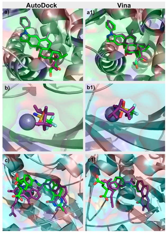
For each target in the DUD–E dataset, an initial analysis of the PDB file associated was performed. The binding pocket was studied and evaluated. Similar PDB structures with co-crystallized ligands were also inspected. Re-docking of the ligands for which there was a ligand-target structure available was performed with AutoDock and with Vina. The docking protocol for both programs was adjusted so as to reproduce the known experimental binding poses for each target, a standard protocol, when validating a docking program/protocol for a specific target [24], as presented in Figure 2. Parameters adjusted in this process with Vina included in the box size and position, number of generated binding modes and exhaustiveness. In AutoDock, the parameters optimized also included the box size and position, number of grid points and spacing, number of genetic algorithm (GA) runs, population size, maximum number of energy evaluations, and maximum number of generations. After the first optimization stage performed for each target, the box dimensions and center coordinates used for both AutoDock and Vina were the same. The exhaustiveness value used for Vina was 8. As for AutoDock, the grid spacing was set to 0.375 Å and the number of GA runs was set to 10. All this information is provided in Table S1 in the Supplementary Materials.

With the current protocol, the computational time for the virtual screening of the complete DUD–E dataset for Vina was of approximately 60 days in 24 CPUs. Calculations in AutoDock took on average 100 times more.

At the end of this stage an optimized docking protocol was selected for each target with each docking program. These protocols were used for the corresponding 101 protein targets to dock the associated ligands and decoys. For each target, ranked lists of ligands and decoys were prepared with AutoDock and Vina, based on the corresponding scores. These lists were used to determine the values of AUCs, EF1% and EF20%, allowing a comparison of the performance of the two docking programs in discriminating between ligands and decoys for each target. Average AUC, EF1% and EF20% were determined for the different families of protein targets and for the full 101 targets.

All protein targets were characterized in terms of the number of the total amino acid residues and molecular weight. The corresponding binding pockets were evaluated in terms of their percentage of hydrophobic, polar, and charged amino acid residues. Average AUC, EF1% and EF20% were determined for different classes of protein targets based on the protein’s size and type of residues at the binding pocket.

The Molecular Operating Environment (MOE) [55] program was used to calculate the chemical and structural properties for all ligands tested. Some of these properties were analyzed in more detail. Examples include the ligand’s molecular weight, volume, area, fraction of rotatable bonds, fraction of hydrophobic accessible surface area (FASA_H), fraction of polar accessible surface area (FASA_P), and fraction of positive and negative accessible surface areas (FASA+ and FASA−). Average AUC, EF(1%) and EF(20%) were also determined for the different classes of ligands based on the ligand’s size, fraction of rotatable bonds and electrostatic nature.

3. Results

3.1. Evaluation of the Performance of AutoDock and Vina

The chemical and structural properties of different proteins and enzymes can vary quite significantly, in features that include the nature, type, and range of interactions around the binding pocket, the pocket size and shape, and the exposure to solvent. Therefore, the challenges that such systems offer to docking and to virtual screening can also be quite different. Some programs and scoring functions are better able to capture some of these characteristics, while other show improved performance in targets with other features.

Table 2. Performance of Vina and AutoDock in the discrimination between ligands and decoys for different classes of targets.

				Vina			AutoDock
Target Class	Targets	Actives	Decoys	EF1%	EF20%	AUC	EF1%	EF20%	AUC
cytochrome P450	2	290	19,242	3.1 ± 0.8	1.4 ± 0.3	57.6 ± 0.6	2.9 ± 1.8	1.0 ± 0.1	50.4 ± 0.4
G protein-coupled receptor	5	1480	99,763	2.8 ± 2.8	1.9 ± 0.9	64.9 ± 6.6	16.6 ± 13.7	3.2 ± 1.3	78.5 ± 15.4
ion channel	2	259	18,379	4.2 ± 3.1	2.6 ± 0.9	66.7 ± 10.3	4.7 ± 3.1	2.8 ± 0.1	75.3 ± 4.4
kinases	23	5065	317,746	13.3 ± 12.0	2.8 ± 0.8	75.2 ± 9.6	5.7 ± 10.2	1.7 ± 0.8	62.1 ± 13.0
nuclear receptor	11	2995	162,175	15.0 ± 8.6	3.0 ± 0.7	73.5 ± 10.4	18.4 ± 13.1	3.3 ± 0.8	79.0 ± 8.8
Proteases	11	3526	208,948	5.3 ± 4.9	2.6 ± 0.7	72.1 ± 8.8	6.9 ± 7.3	1.7 ± 0.9	59.6 ± 10.0
other	29	4663	276,475	9.3 ± 8.9	2.3 ± 1.0	69.6 ± 12.9	6.8 ± 8.3	2.1 ± 1.2	65.1 ± 16.0
metalloenzymes	18	4154	277,785	8.2 ± 10.1	2.2 ± 1.1	64.6 ± 15.1	8.8 ± 10.7	2.2 ± 1.3	61.2 ± 21.9
non-metalloenzymes	83	18,278	1,102,728	10.0 ± 9.6	2.6 ± 0.9	71.4 ± 10.9	8.51 ± 10.5	2.2 ± 1.1	66.1 ± 14.7
Total/Average	101	22,432	1,380,513	7.6 ± 4.7	2.4 ± 0.5	68.0 ± 5.8	8.9 ± 5.6	2.3 ± 0.8	66.4 ± 10.2

compares the performance of AutoDock and Vina across the different classes of targets. The average results obtained for the set of 101 target showed that AutoDock and Vina exhibit a similar average performance in discriminating between ligands and decoys. In fact, the average EF1% values obtained were 7.6 and 8.9 for Vina and AutoDock, respectively (AUCs of 68.0 and 66.4). The EF1% values calculated for this extended data set show that these programs are able to rank in the top 1% of the total ligands (active and decoys) docked against each target, 7.6- and 8.9-times more active ligands than what would be expected from random selection, considering the relative percentage of actives and decoys available for each target.

However, the discrimination ability across different target classes could vary significantly. For GPCRs, for example, AutoDock exhibited superior discrimination ability, with an average EF1% of 16.6 against only 2.8 with VINA. AutoDock also demonstrated improved performance over Vina for Nuclear Receptors (EF1% of 18.4 versus 15.0). However, for kinases and metalloproteins the discrimination ability of Vina is on average better than that of AutoDock.

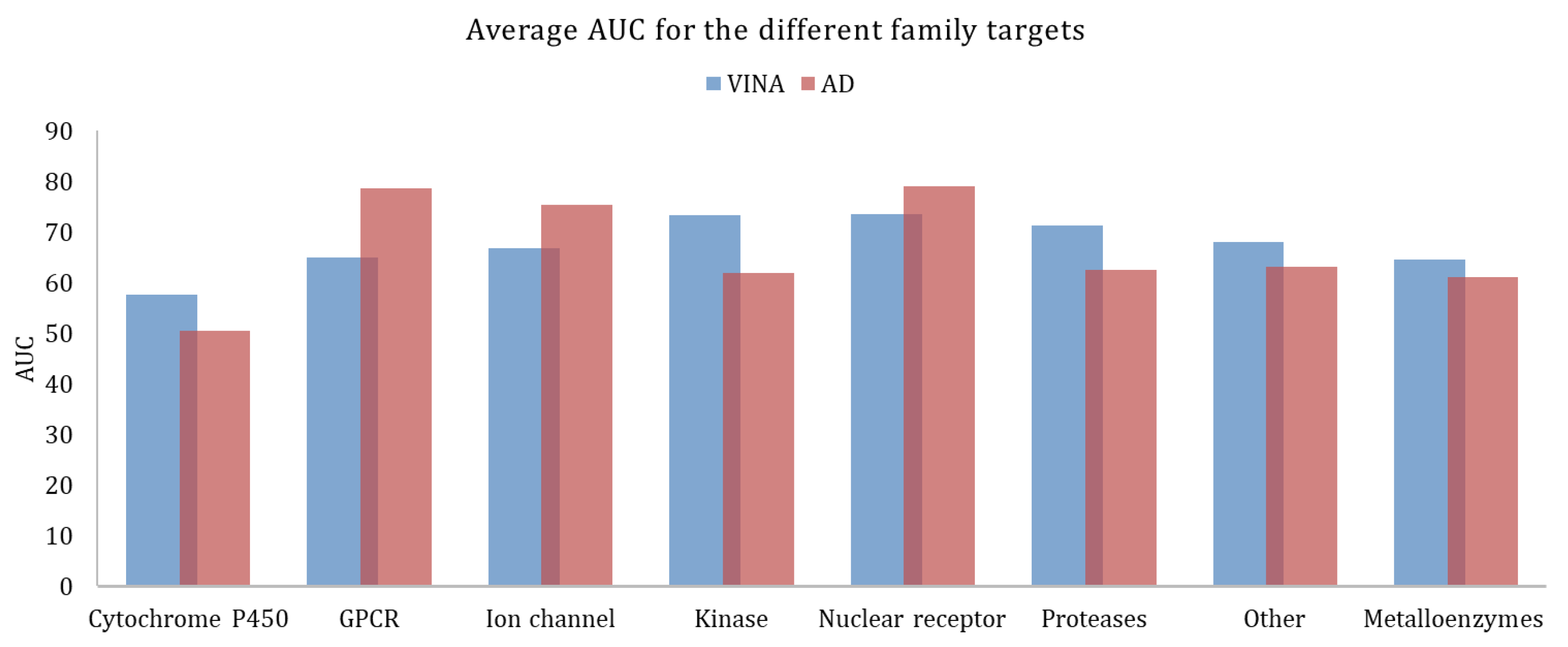
Figure 3, shows the average AUC values, calculated for the different target families. As previously mentioned, the higher the AUC, the better the discrimination ability between actives and decoys. AutoDock provided better results for GPCRs, ion channels, and nuclear receptors. Vina worked better for all the other families.

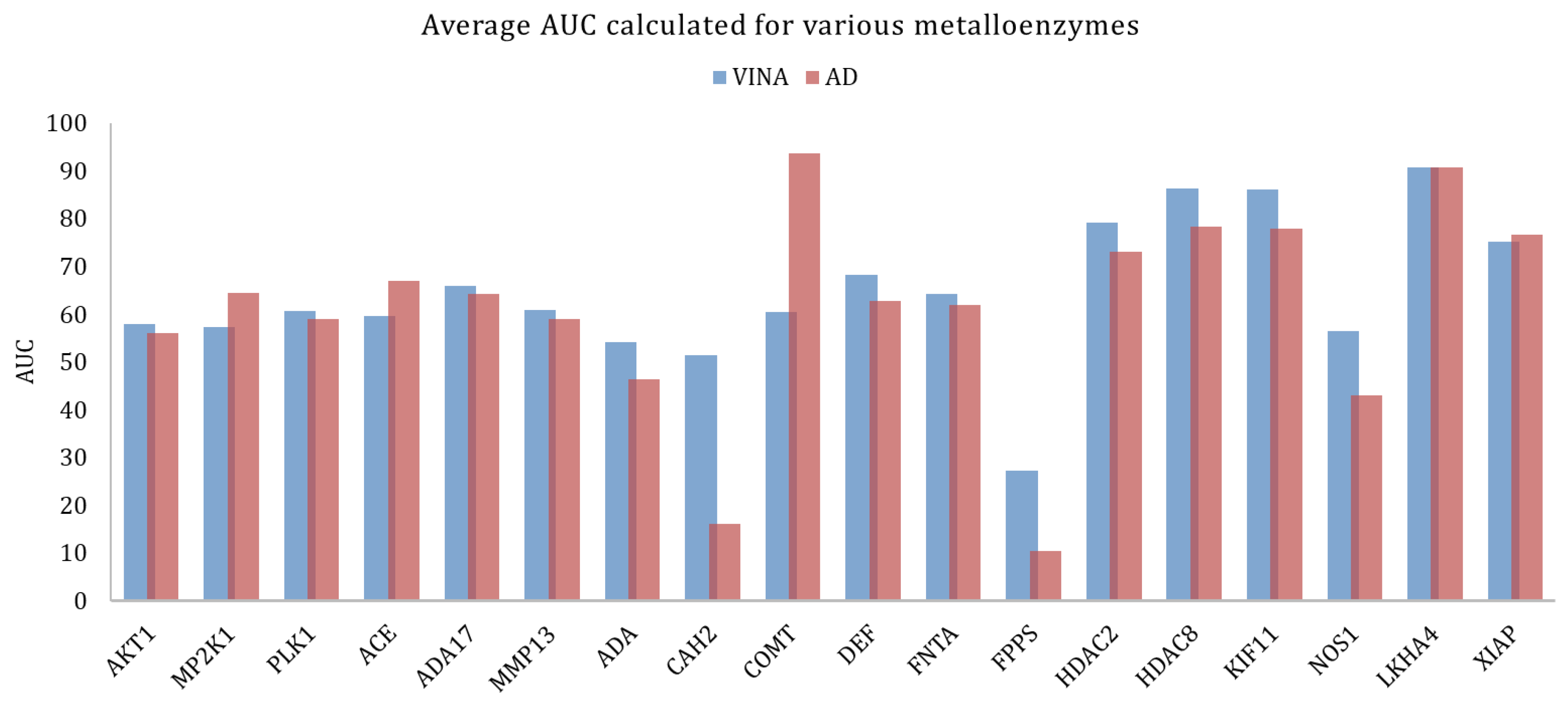
However, across large families of proteins there could be significant variations in the docking results, when looking into individual proteins. In the case of metalloenzymes, for example, Vina provided better results, on average. Analyzing each target in particular (Figure 4) it could be seen that for some targets the AutoDock performed significantly better. This might be explained by the fact that in this family there is a large variability of types of proteins as this group includes kinases, proteases, and others.

Table 3. Performance of Vina and AutoDock in the discrimination between ligands and decoys for the targets of different sizes based on the number of amino acid residues of each target (number of aa).

Target Size (Number of aa)	Vina		AutoDock
	EF1%	AUC	EF1%	AUC
Small (0–250 aa)	8.6 ± 10.1	70.7 ± 11.0	9.4 ± 12.3	66.6 ± 16.0
Medium (250–400 aa)	11.5 ± 10.0	71.8 ± 12.5	7.9 ± 9.7	64.3 ± 15.8
Large (>400 aa)	6.1 ± 7.0	65.4 ± 11.0	8.9 ± 10.6	65.8 ± 18.2

analyzes the performance of AutoDock and VINA taking into consideration the number of amino acid residues that constitute the target. For smaller targets, the driving force for ligand-binding tends to be more concentrated in a smaller number of key specific residues. Additionally, the binding pockets tended to be smaller, or often more exposed to the solvent. On the other hand, in larger protein-targets, the range of interactions involved in ligand-binding tended to be larger and more diffused. In addition, the extra number of amino acid residues present in the larger targets could confer a more controlled environment to the corresponding binding pockets, shielding the interactions formed from the effect of the solvent. The non-specific protein environment could play a more important role for ligand-binding in these targets. Therefore, the number of amino acid residues that constituted the different targets could offer different trials for docking and virtual screening.

The results from Table 3 show that Vina was, on average, better in discriminating ligands from decoys in medium-sized targets, with 250 to 400 amino acid residues (average EF1% of 11.5, AUC 71.8). For targets with more than 400 amino acid residues, the performance of Vina was significantly lower (average EF1% of only 6.1, AUC of 65.4)

AutoDock exhibited a more uniform behavior, with average EF1% values in the range 7.9–9.4 for small (less than 250 aa) and large targets (more than 400 aa), resulting in an improved performance over Vina for the small targets (<250 aa) and the large targets (>400 aa).

Another important aspect regarding the nature of the target protein concerns the type of amino acid residues that constitute each binding pocket. For this analysis, all amino acid residues defining each binding pocket were grouped into polar, charged (negative and positive), and hydrophobic amino acid residues. Binding pockets were characterized based on the relative percentage of each of these types of residues. Average EF1% and AUC values were calculated with AutoDock and Vina for each category. The results are presented in

Table 4. Performance of Vina and AutoDock in the discrimination between ligands and decoys for targets with binding pockets with different percentages of polar, charged, and hydrophobic amino acid residues.

		Vina		AutoDock
Polarity	Number of Targets	EF1%	AUC	EF1%	AUC
Poorly Polar (0–25%)	25	9.9 ± 8.86	68.1 ± 12.9	11.7 ± 12.5	68.7 ± 15.7
Moderately Polar (25–35%)	36	10.7 ± 9.32	71.7 ± 11.7	8.0 ± 9.5	63.7 ± 16.4
Very Polar (>35%)	40	8.6 ± 10.6	70.0 ± 13.1	7.0 ± 9.8	64.2 ± 16.5
Hydrophobicity
Poorly Hydrophobic (0–30%)	38	11.1 ± 11.5	72.4 ± 13.4	8.5 ± 10.1	66.7 ± 17.2
Moderately Hydrophobic (30–40%)	25	8.3 ± 8.5	68.4 ± 13.3	8.2 ± 13.3	62.9 ± 18.1
Very Hydrophobic (>40%)	38	9.1 ± 8.4	69.0 ± 9.3	8.8 ± 9.3	65.0 ± 14.2
Charge
Poorly Charged (0–15%)	40	9.9 ± 9.1	69.2 ± 11.4	10.2 ± 10.9	68.8 ± 15.5
Moderately Charged (15–20%)	24	7.7 ± 8.6	68.2 ± 11.9	5.8 ± 8.7	55.1 ± 17.5
Very Charged (>20%)	37	10.7 ± 10.9	72.4 ± 12.7	8.5 ± 10.9	67.5 ± 13.8
Positive Charge
Poorly Positive (0–5%)	24	10.2 ± 8.5	67.9 ± 11.6	12.6 ± 11.6	68.8 ± 15.6
Moderately Positive (5–10%)	34	8.5 ± 10.8	69.6 ± 14.2	6.9 ± 11.1	62.1 ± 17.5
Very Positive (>10%)	43	10.5 ± 9.4	72.6 ± 9.7	7.9 ± 8.8	65.4 ± 15.3
Negative Charge
Poorly Negative (0–5%)	22	11.0 ± 9.5	70.8 ± 9.8	11.7 ± 10.7	73.5 ± 11.9
Moderately Negative (5–10%)	44	8.1 ± 8.3	70.2 ± 11.8	7.2 ± 10.2	62.2 ± 17.4
Very Negative (>10%)	35	10.9 ± 11.2	69.7 ± 13.8	8.2 ± 10.7	63.5 ± 10.7

.

The results presented in Table 4 showed that for poorly polar binding pockets (less than 25% of polar residues) AutoDock was on average better than Vina in discriminating between ligands and decoys, particularly among the top 1% of ranked solutions. For moderately polar and very polar binding pockets, Vina exhibited a better performance than AutoDock. The results also showed that both programs had more difficulty in discriminating ligands and decoys for very polar binding pockets (>35% of polar amino acid residues).

In terms of the percentage of hydrophobic residues, the results showed that Vina was significantly better than AutoDock in ligand/decoy discrimination for poorly hydrophobic binding pockets. As the percentage of hydrophobic residues at the binding pocket increased, the performance of Vina and AutoDock became increasingly similar, both in terms of EC1% and in terms of AUC values.

In terms of charge, the results showed that AutoDock was better in discriminating ligands and decoys in poorly charged binding pockets (<15%) than in moderate or highly charged ones. Vina, on the other hand, gave best results in highly charged binding pockets. These general tendencies concerning the presence of a charge at the binding pocket were also observed when particularly looking into positively charged residues or into negatively charged residues.

In general, these results showed that AutoDock was better in discriminating ligands and decoys in more hydrophobic, poorly polar, and poorly charged pockets, while Vina exhibited early recognition metrics that did not vary so significantly with the type of amino acid residues at the binding pocket. Vina tended to give better results for polar and charged binding pockets, which was particularly interesting, taking into consideration that the scoring function of Vina did not explicitly include charges, while that of AutoDock had an explicit electrostatic term.

3.2. Substrates

The type of molecule to be evaluated and its physico-chemical characteristics also offer different challenges for virtual screening, in terms of docking and its ability to discriminate between actives and decoys. For each specific target, the decoys included in the DUD–E were generated by having similar 1-D physico-chemical properties to the actives from which they originated, to remove bias [32]. Hence, to analyze how the different substrate properties affected the discriminating ability of each target, the physical properties of all actives identified in the ligands ranked as the top 1% were evaluated and compared with the other actives that were ranked the worst.

In this study, four fundamental properties of the ligands were analyzed—the size of the ligands, polarity, charge, and the number of rotatable bonds.

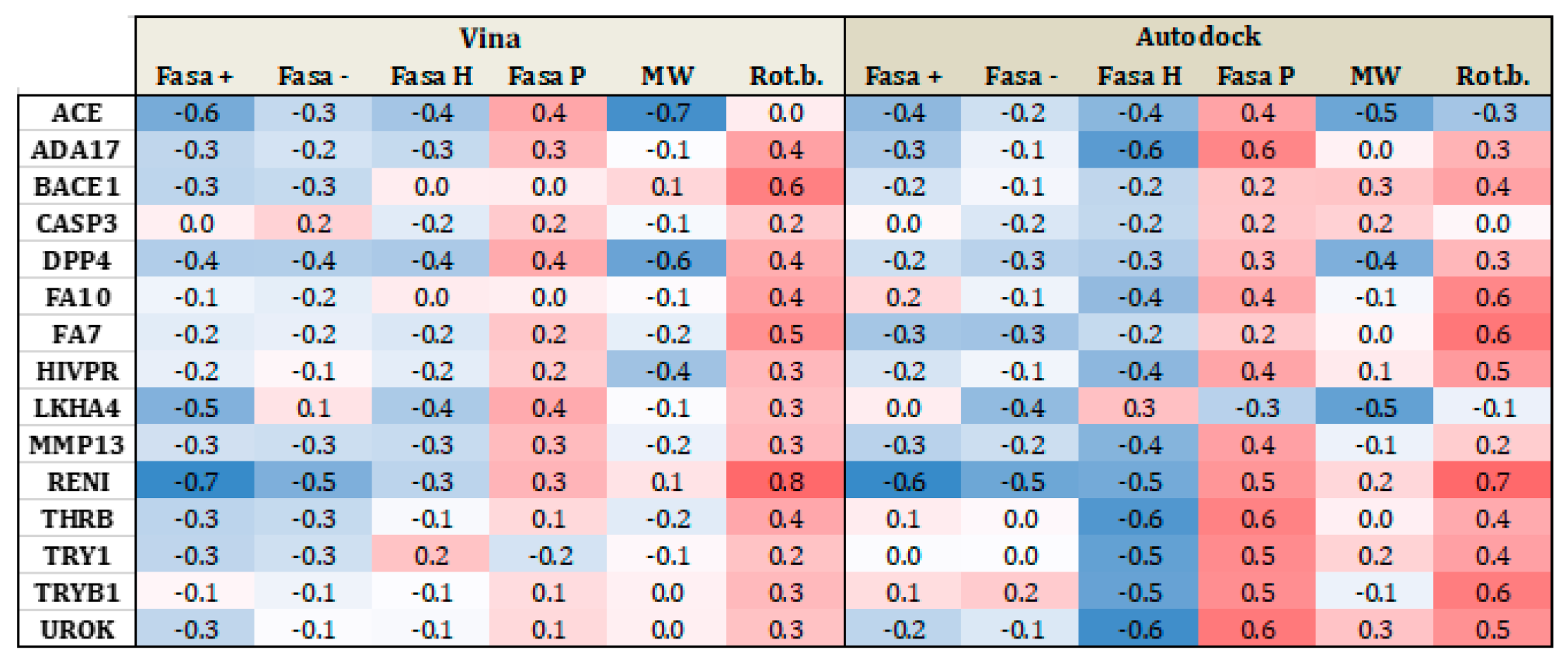
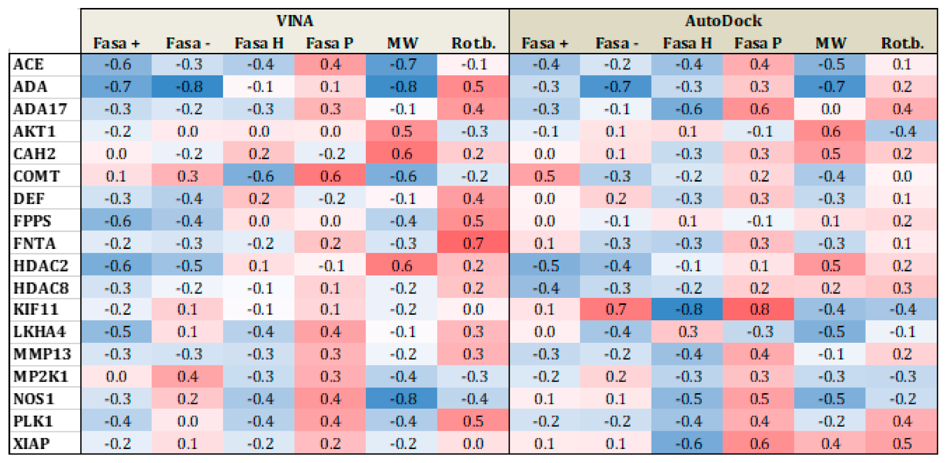
Figure 5 and Figure 6 present heat maps of the correlation between the substrate properties and their position in the ranking according to the type of target family (proteases and metalloenzymes, respectively). Darker red (+1) yield perfect positive correlation while darker blue (−1), yield perfect negative correlation. From Figure 5, it is clear that polarity and number of rotational bonds is important for both Vina and is even more distinct for AutoDock, since it presents a positive correlation, that is, as the ranking number increases, the polarity and number of rotational bonds also increase. This means that the molecules with more rotatable bonds and which are more polar, are ranked worst in the list. This leads to the conclusion that more polar and more flexible molecules present a bigger challenge for AutoDock, in particular. For metalloenzymes, the correlation profile is a little bit different from proteases. It is not easy to find a clear tendency because while some targets present a positive correlation for some property, others have a negative correlation for the same property. This could again be explained by the large variability of protein types in this particular family.

3.1.1. Influence of Molecular Weight

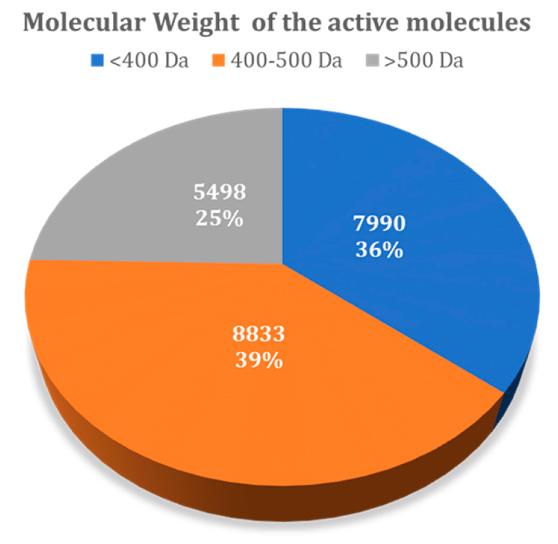
Figure 7 summarizes the variability of all molecules present in the DUD–E dataset, taking into account the molecular weight. The results showed that from the total of 22,321 active ligands considered for all 101 DUD–E targets, 7990 have a molecular weight below 400 Da, while 8833 have a molecular weight in the range of 400–500 Da, with 5498 with a molecular weight over 500 Da. The distribution of decoys across these ranges was the same, as they were generated automatically from the known ligands included.

Table 5. Influence of the molecular weight for actives found in the top 1% of the database.

	Vina	AutoDock
	No. of Ligands within Top 1%	No. of Ligands within Top 1%
Total	2002 (8.9%)	1935 (8.6%)
<400 Da	536 (2.4%)	395 (1.8%)
400–500 Da	885 (3.9%)	1043 (4.7%)
>500 Da	581 (2.6%)	497 (2.2%)

decomposes the number of ligands identified in the top 1% of compounds ranked, according to the molecular weight. AutoDock identified a total of 1935 actives in the top 1% of ligands, while in Vina, this number was of 2002. The results showed that Vina was, on average, better than AutoDock in identifying actives in the top 1% of small ligands (<400 MW) (536 versus 395 actives) and for large-sized ligands (>500 MW) (581 versus 497 actives). However, AutoDock was able to rank more medium-sized actives (400–500 MW) among the top 1% of the results (1043 versus 885).

Regarding each family of proteins, all exhibited the same tendency—smaller ligands were more difficult to discriminate and appeared at worst ranking positions for both Vina and AutoDock.

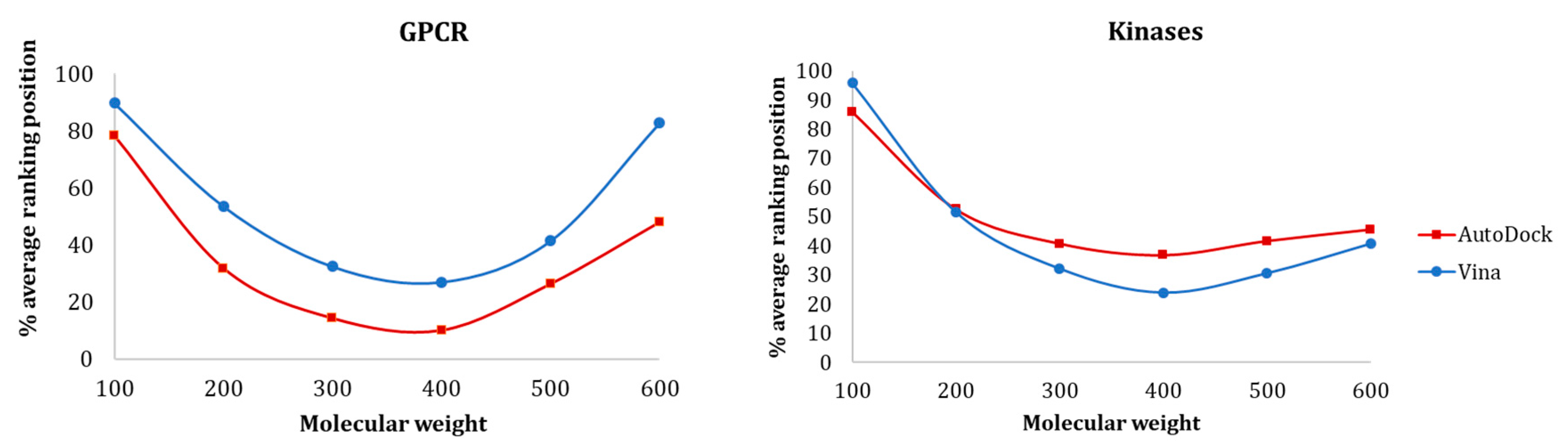
Figure 8 shows the influence of molecular weight on the average ranking distribution of the molecules within the full-ranked list determined for each protein target. The results showed that there was a similar tendency for both GPCR and kinase protein families, where the smaller ligands were ranked worst and the medium ligands were ranked better. For both GPCRs and kinases, AutoDock could rank smaller ligands better than Vina, even though their ranking position was relatively high. As for the medium-sized active molecules (300–400), these two families exhibited opposite results—while Vina provided better recognition for kinases, AutoDock was more effective in discriminating actives and decoys for GPCRs.

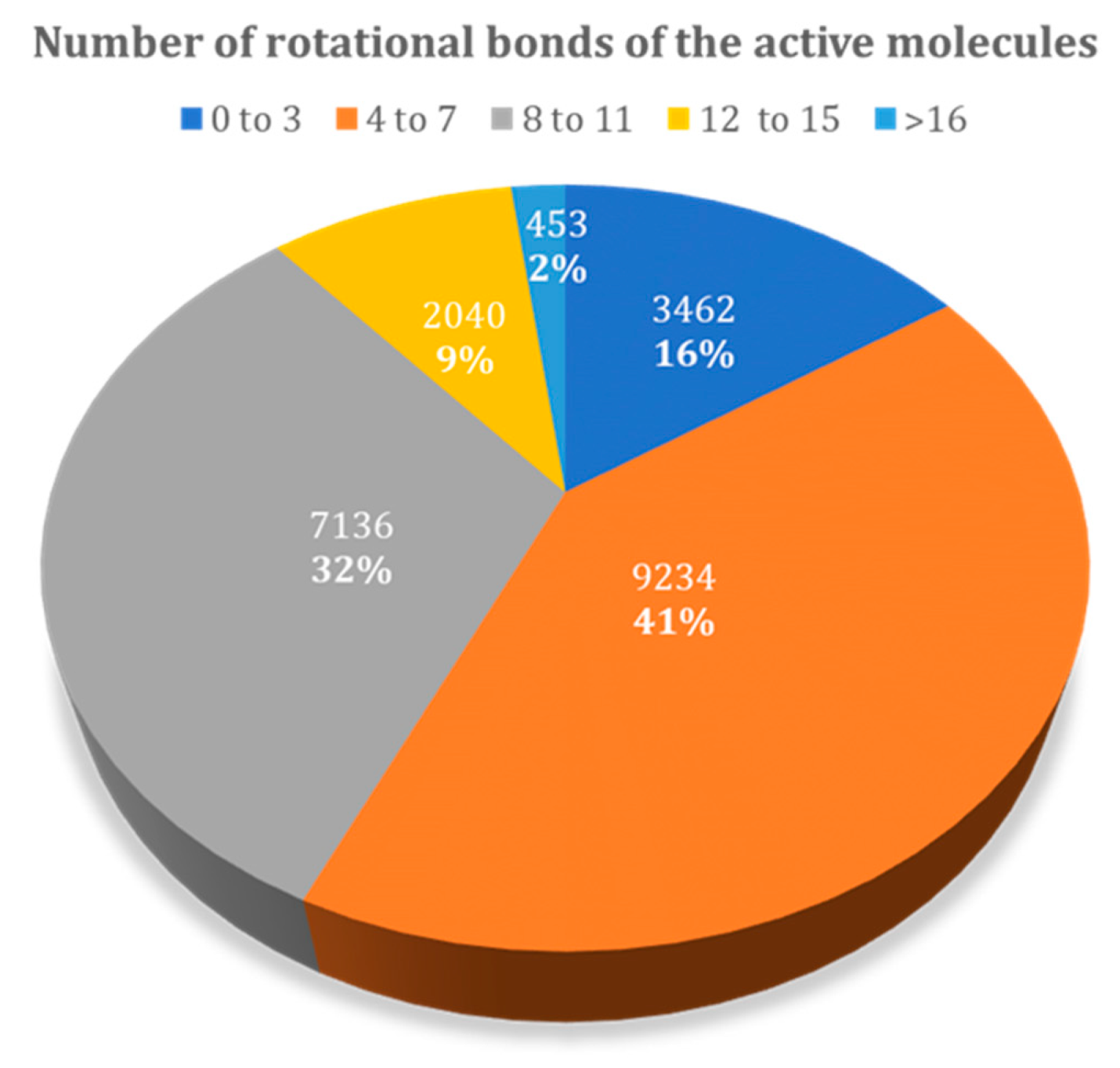
3.1.2. Influence of the Number of Rotational Bonds

Figure 9 presents the relative distribution of all active ligands in the DUD–E dataset taking into consideration the number of rotational bonds present. There is a higher prevalence in molecules with 4 to 7, and 8 to 11 rotational bonds, representing 73% of the dataset. The remaining 27% corresponds to molecules with 0 to 3 and higher than 12 rotational bonds.

Ligands with more rotatable bonds presented a higher challenge for docking because they could adopt a larger number of possible conformations. Discriminating actives with many rotatable bonds from decoys with many rotatable bonds hence became more difficult, because correctly identifying the real pose of the ligand was more challenging. Hence, ligands with a higher number of rotational bonds were placed at the worst position in the database, when comparing with the ligands with fewer rotatable bonds. In this study, this was observed for all studied families.

In Figure 10, the data for nuclear receptors and GPCRs are presented. For both families, AutoDock was able to rank more ligands early on. While in GPCRs there was a clear difference in the discrimination ability between Vina and AutoDock, for nuclear receptors, there was a similar behavior between both alternatives (exception—compounds with 4 rotatable bonds in nuclear receptors). According to our study, molecules with 5 to 10 rotational bonds ensured a better prediction with both AutoDock and Vina.

4. Discussion

AutoDock and Vina are efficient software alternatives for virtual screening, exhibiting on average similar performance when evaluating the ligand/decoy discriminating ability, across a large number of proteins. In spite of the similar average performance exhibited, both docking programs can present a marked difference when studying a particular protein target, or even when looking into proteins or enzymes from specific families, or for different types of ligands. Hence, for the common user wishing to embark in a virtual screening study, it is not easy to select a priori the alternative that should be used.

The goal of this study was to guide the selection of the docking software according to the type and characteristics of the target and its substrates. As demonstrated, the type of target, and specially the characteristics of the binding pocket could influence the outcome of the docking software. The results showed that AutoDock was clearly better in discriminating ligands and decoys in smaller targets, with more hydrophobic, poorly polar, and poorly charged pockets, while Vina tended to give better results for bigger targets with polar and charged binding pockets. According to the results presented, Vina provided better metrics for kinases, proteases, and cytochrome P450. On the other hand, ligand/decoy discrimination for GPCR, ion channels, and nuclear receptors was improved with AutoDock.

For the substrates, however, this analysis across 22,432 active compounds and 1,380,513 decoy molecules showed that AutoDock and Vina exhibited comparable trends with the ligands size, charge, and the number of rotatable bonds. Bigger, more flexible, and more polar ligands were more difficult to discriminate from decoys for both docking programs but the performance of Vina and AutoDock was quite similar.

5. Conclusions

While the present study offered useful guidelines that could help researchers to choose between AutoDock or Vina before starting a new virtual screening, according to the characteristics of their specific target, it also highlighted another important aspect. The performance of both programs could in some cases vary significantly, even for very similar proteins. Therefore, for very specific systems, it is recommended that researchers test both alternatives wisely, before starting a large virtual screening study.

References

- Kitchen, D.B.; Decornez, H.; Furr, J.R.; Bajorath, J. Docking and Scoring in Virtual Screening for drug discovery: Methods and applications. Nat. Rev. Drug Discov. 2004, 3, 935–949. [Google Scholar] [CrossRef] [PubMed]
- Kinnings, S.L.; Liu, N.; Buchmeier, N.; Tonge, P.J.; Xie, L.; Bourne, P.E. Drug discovery using chemical systems biology: Repositioning the safe medicine Comtan to treat multi-drug and extensively drug resistant tuberculosis. PLoS Comput. Biol. 2009, 5, e1000423. [Google Scholar] [CrossRef]
- Ma, D.L.; Chan, D.S.H.; Leung, C.H. Drug repositioning by structure-based virtual screening. Chem. Soc. Rev. 2013, 42, 2130–2141. [Google Scholar] [CrossRef] [PubMed]
- Govindaraj, R.G.; Naderi, M.; Singha, M.; Lemoine, J.; Brylinski, M. Large-scale computational drug repositioning to find treatments for rare diseases. NPJ Syst. Biol. Appl. 2018, 4, 1–10. [Google Scholar] [CrossRef] [PubMed]
- Sousa, F.S.; Fernandes, P.A.; Ramos, M.J. Protein—Ligand Docking: Current Status and Future Challenges. Proteins Struct. Funct. Bioinforma 2006, 26, 15–26. [Google Scholar] [CrossRef]
- Sousa, S.F.; Cerqueira, N.M.F.S.A.; Fernandes, P.A.; Ramos, M.J. Virtual screening in drug design and development. Comb. Chem. High Throughput Screen. 2010, 13, 442–453. [Google Scholar] [CrossRef]
- Lohning, A.E.; Levonis, S.M.; Williams-Noonan, B.; Schweiker, S.S. A Practical Guide to Molecular Docking and Homology Modelling for Medicinal Chemists. Curr. Top. Med. Chem. 2017, 17, 2023–2040. [Google Scholar] [CrossRef] [Green Version]
- Sousa, S.F.; Ribeiro Antonio, J.M.; Coimbra, J.T.S.; Neves, R.P.P.; Martins, S.A.; Moorthy, N.S.H.N.; Fernandes, P.A.; Ramos, M.J. Protein-Ligand Docking in the New Millennium—A Retrospective of 10 Years in the Field. Curr. Med. Chem. 2013, 20, 2296–2314. [Google Scholar] [CrossRef]
- Ferreira, L.G.; Dos Santos, R.N.; Oliva, G.; Andricopulo, A.D. Molecular docking and structure-based drug design strategies. Molecules 2015, 20, 13384–13421. [Google Scholar] [CrossRef]
- Kroemer, R.T. Structure-based drug design: Docking and scoring. Curr. Protein Pept. Sci. 2007, 8, 312–328. [Google Scholar] [CrossRef]
- Taylor, R.D.; Jewsbury, P.J.; Essex, J.W. A review of protein-small molecule docking methods. J. Comput. Aided Mol. Des. 2002, 16, 151–166. [Google Scholar] [CrossRef] [PubMed]
- Huang, S.; Zou, X. Advances and challenges in Protein-ligand docking. Int. J. Mol. Sci. 2010, 11, 3016–3034. [Google Scholar] [CrossRef] [PubMed]
- Zhou, Z.; Cheng, T.; Li, Q.; Bryant, S.H.; Wang, Y. Structure-Based Virtual Screening for Drug Discovery: A Problem-Centric Review. AAPS J. 2012, 14, 133–141. [Google Scholar]
- Ban, T.; Ohue, M.; Akiyama, Y. Multiple grid arrangement improves ligand docking with unknown binding sites: Application to the inverse docking problem. Comput. Biol. Chem. 2018, 73, 139–146. [Google Scholar] [CrossRef] [PubMed]
- Totrov, M.; Abagyan, R. Flexible ligand docking to multiple receptor conformations: A practical alternative. Curr. Opin. Struct. Biol. 2008, 18, 178–184. [Google Scholar] [CrossRef]
- Huang, S.-Y. Comprehensive assessment of flexible-ligand docking algorithms: Current effectiveness and challenges. Brief. Bioinform. 2018, 19, 982–994. [Google Scholar] [CrossRef]
- Kong, X.; Sun, H.; Pan, P.; Zhu, F.; Chang, S.; Xu, L.; Li, Y.; Hou, T. Importance of protein flexibility in molecular recognition: A case study on Type-I1/2 inhibitors of ALK. Phys. Chem. Chem. Phys. 2018, 20, 4851–4863. [Google Scholar] [CrossRef]
- Sahai, M.A.; Biggin, P.C. Quantifying water-mediated protein-ligand interactions in a glutamate receptor: A DFT study. J. Phys. Chem. B 2011, 115, 7085–7096. [Google Scholar] [CrossRef]
- Munawar, S.; Vandenberg, J.I.; Jabeen, I. Molecular Docking Guided Grid-Independent Descriptor Analysis to Probe the Impact of Water Molecules on Conformational Changes of hERG Inhibitors in Drug Trapping Phenomenon. Int. J. Mol. Sci. 2019, 20, 3385. [Google Scholar] [CrossRef]
- Rentzsch, R.; Renard, B.Y. Docking small peptides remains a great challenge: An assessment using AutoDock Vina. Brief. Bioinform. 2015, 16, 1045–1056. [Google Scholar] [CrossRef]
- Hauser, A.S.; Windshügel, B. LEADS-PEP: A Benchmark Data Set for Assessment of Peptide Docking Performance. J. Chem. Inf. Model. 2016, 56, 188–200. [Google Scholar] [CrossRef] [PubMed]
- Isa, D.M.; Chin, S.P.; Chong, W.L.; Zain, S.M.; Rahman, N.A.; Lee, V.S. Dynamics and binding interactions of peptide inhibitors of dengue virus entry. J. Biol. Phys. 2019, 45, 63–76. [Google Scholar] [CrossRef] [PubMed]
- Cerqueira, N.M.; Gesto, D.; Oliveira, E.F.; Santos-Martins, D.; Brás, N.F.; Sousa, S.F.; Fernandes, P.A.; Ramos, M.J. Receptor-based virtual screening protocol for drug discovery. Arch. Biochem. Biophys. 2015, 582, 56–67. [Google Scholar] [CrossRef] [PubMed]
- Ramírez, D.; Caballero, J. Is it reliable to use common molecular docking methods for comparing the binding affinities of enantiomer pairs for their protein target? Int. J. Mol. Sci. 2016, 17, 525. [Google Scholar] [CrossRef]
- Muegge, I.; Rarey, M. Small Molecule Docking and Scoring. In Reviews in Computational Chemistry; Kenny Lipkowitz, K.B., Boyd, D.B., Eds.; John Wiley & Sons, Inc.: Hoboken, NJ, USA, 2001; Volume 17, pp. 1–60. [Google Scholar]
- Cole, J.C.; Murray, C.W.; Nissink, J.W.M.; Taylor, R.D.; Taylor, R. Comparing protein-ligand docking programs is difficult. Proteins Struct. Funct. Bioinform. 2005, 60, 325–332. [Google Scholar] [CrossRef]
- Kontoyianni, M.; McClellan, L.M.; Sokol, G.S. Evaluation of Docking Performance: Comparative Data on Docking Algorithms. J. Med. Chem. 2004, 47, 558–565. [Google Scholar] [CrossRef]
- Xu, W.; Lucke, A.J.; Fairlie, D.P. Comparing sixteen scoring functions for predicting biological activities of ligands for protein targets. J. Mol. Graph. Model. 2015, 57, 76–88. [Google Scholar] [CrossRef] [Green Version]
- Wang, Z.; Sun, H.; Yao, X.; Li, D.; Xu, L.; Li, Y.; Tian, S.; Hou, T. Comprehensive evaluation of ten docking programs on a diverse set of protein-ligand complexes: The prediction accuracy of sampling power and scoring power. Phys. Chem. Chem. Phys. 2016, 18, 12964–12975. [Google Scholar] [CrossRef]
- Vieira, T.F.; Magalhaes, R.; Sousa, S.F. Tailoring specialized scoring functions for more efficient virtual screening. Front. Drug, Chem. Clin. Res. 2019, 2, 1–4. [Google Scholar]
- Mysinger, M.M.; Carchia, M.; Irwin, J.J.; Shoichet, B.K. Directory of Useful Decoys, Enhanced (DUD-E): Better Ligands and Decoys for Better Benchmarking. J. Med. Chem. 2012, 55, 6582–6594. [Google Scholar] [CrossRef]
- Bartuzi, D.; Kaczor, A.; Targowska-Duda, K.; Matosiuk, D. Recent Advances and Applications of Molecular Docking to G Protein-Coupled Receptors. Molecules 2017, 22, 340. [Google Scholar] [CrossRef] [PubMed]
- Seong, S.H.; Ali, M.Y.; Kim, H.-R.; Jung, H.A.; Choi, J.S. BACE1 inhibitory activity and molecular docking analysis of meroterpenoids from Sargassum serratifolium. Bioorg. Med. Chem. 2017, 25, 3964–3970. [Google Scholar] [CrossRef] [PubMed]
- Nisha, C.M.; Kumar, A.; Vimal, A.; Bai, B.M.; Pal, D.; Kumar, A. Docking and ADMET prediction of few GSK-3 inhibitors divulges 6-bromoindirubin-3-oxime as a potential inhibitor. J. Mol. Graph. Model. 2016, 65, 100–107. [Google Scholar] [CrossRef] [PubMed]
- Ravindranath, P.A.; Forli, S.; Goodsell, D.S.; Olson, A.J.; Sanner, M.F. AutoDockFR: Advances in Protein-Ligand Docking with Explicitly Specified Binding Site Flexibility. PLoS Comput. Biol. 2015, 11, e1004586. [Google Scholar] [CrossRef] [PubMed]
- Labbé, C.M.; Rey, J.; Lagorce, D.; Vavrusa, M.; Becot, J.; Sperandio, O.; Villoutreix, B.O.; Tufféry, P.; Miteva, M.A. MTiOpenScreen: A web server for structure-based virtual screening. Nucleic Acids Res. 2015, 43, W448–W454. [Google Scholar] [CrossRef] [PubMed]
- Koebel, M.R.; Schmadeke, G.; Posner, R.G.; Sirimulla, S. AutoDock VinaXB: Implementation of XBSF, new empirical halogen bond scoring function, into AutoDock Vina. J. Cheminform. 2016, 8, 27. [Google Scholar] [CrossRef]
- Quiroga, R.; Villarreal, M.A. Vinardo: A scoring function based on autodock vina improves scoring, docking, and virtual screening. PLoS ONE 2016, 11, e0155183. [Google Scholar] [CrossRef]
- Di Muzio, E.; Toti, D.; Polticelli, F. DockingApp: A user-friendly interface for facilitated docking simulations with AutoDock Vina. J. Comput. Aided Mol. Des. 2017, 31, 213–218. [Google Scholar] [CrossRef]
- Morris, G.M.; Huey, R.; Lindstrom, W.; Sanner, M.F.; Belew, R.K.; Goodsell, D.S.; Olson, A.J. Software news and updates AutoDock4 and AutoDockTools4: Automated docking with selective receptor flexibility. J. Comput. Chem. 2009, 30, 2785–2791. [Google Scholar] [CrossRef]
- Morris, G.M.; Goodsell, D.S.; Huey, R.; Olson, A.J. Distributed automated docking of flexible ligands to proteins: Parallel applications of AutoDock 2.4. J. Comput. Aided Mol. Des. 1996, 10, 293–304. [Google Scholar] [CrossRef]
- Goodsell, D.S.; Morris, G.M.; Olson, A.J. Automated docking of flexible ligands: Applications of AutoDock. J. Mol. Recognit. 1996, 9, 1–5. [Google Scholar] [CrossRef]
- Morris, G.M.; Goodsell, D.S.; Halliday, R.S.; Huey, R.; Hart, W.E.; Belew, R.K.; Olson, A.J. Automated Docking Using a Lamarckian Genetic Algorithm and an Empirical Binding Free Energy Function. J. Comput. Chem. 1998, 19, 1639–1662. [Google Scholar] [CrossRef]
- Trott, O.; Olson, A.J. AutoDock Vina: Improving the speed and accuracy of docking with a new scoring function, efficient optimization and multithreading. J. Comput. Chem. 2010, 31, 455–461. [Google Scholar] [CrossRef] [PubMed]
- Jaghoori, M.M.; Bleijlevens, B.; Olabarriaga, S.D. 1001 Ways to run AutoDock Vina for virtual screening. J. Comput. Aided Mol. Des. 2016, 30, 237–249. [Google Scholar] [CrossRef] [PubMed]
- Coleman, R.G.; Carchia, M.; Sterling, T.; Irwin, J.J.; Shoichet, B.K. Ligand Pose and Orientational Sampling in Molecular Docking. PLoS ONE 2013, 10, e75992. [Google Scholar] [CrossRef]
- Allen, W.J.; Balius, T.E.; Mukherjee, S.; Brozell, S.R.; Moustakas, D.T.; Lang, P.T.; Case, D.A.; Kuntz, I.D.; Rizzo, R.C. DOCK 6: Impact of new features and current docking performance. J. Comput. Chem. 2015, 36, 1132–1156. [Google Scholar] [CrossRef] [Green Version]
- Chaput, L.; Martinez-Sanz, J.; Saettel, N.; Mouawad, L. Benchmark of four popular virtual screening programs: Construction of the active/decoy dataset remains a major determinant of measured performance. J. Cheminform. 2016, 8, 1–17. [Google Scholar] [CrossRef]
- Uehara, S.; Tanaka, S. AutoDock-GIST: Incorporating Thermodynamics of Active-Site Water into Scoring Function for Accurate Protein-Ligand Docking. Molecules 2016, 21, 1604. [Google Scholar] [CrossRef]
- Ericksen, S.S.; Wu, H.; Zhang, H.; Michael, L.A.; Newton, M.A.; Hoffmann, F.M.; Wildman, S.A. Machine Learning Consensus Scoring Improves Performance Across Targets in Structure-Based Virtual Screening. J. Chem. Inf. Model. 2017, 57, 1579–1590. [Google Scholar] [CrossRef] [Green Version]
- Zhou, H.; Cao, H.; Skolnick, J. FINDSITE comb2.0: A New Approach for Virtual Ligand Screening of Proteins and Virtual Target Screening of Biomolecules. J. Chem. Inf. Model. 2018, 58, 2343–2354. [Google Scholar] [CrossRef]
- Ebejer, J.P.; Finn, P.W.; Wong, W.K.; Deane, C.M.; Morris, G.M. Ligity: A Non-Superpositional, Knowledge-Based Approach to Virtual Screening. J. Chem. Inf. Model. 2019, 59, 2600–2616. [Google Scholar] [CrossRef] [PubMed] [Green Version]
- Wang, D.; Cui, C.; Ding, X.; Xiong, Z.; Zheng, M.; Luo, X.; Jiang, H.; Chen, K. Improving the Virtual Screening Ability of Target-Specific Scoring Functions Using Deep Learning Methods. Front. Pharmacol. 2019, 10. [Google Scholar] [CrossRef] [PubMed]
- Chen, P.; Ke, Y.; Lu, Y.; Du, Y.; Li, J.; Yan, H.; Zhao, H.; Zhou, Y.; Yang, Y. DLIGAND2: An improved knowledge-based energy function for protein–ligand interactions using the distance-scaled, finite, ideal-gas reference state. J. Cheminform. 2019, 11, 52. [Google Scholar] [CrossRef] [PubMed]
- Molecular Operating Environment (MOE), 2013.08; Chemical Computing Group ULC, Montreal, Canada. 2019. Available online: https://www.chemcomp.com/index.htm (accessed on 18 October 2019).
Figure 1.
Overview of the protein target families of the Directory of Useful Decoys–Enhanced (DUD–E) dataset.
Figure 2.
Comparison between the crystallographic (green) and “docked” (purple) poses of (a) glucocorticoid receptor (GCR) Autodock, (a1) GCR Vina, (b) CAH2 AutoDock, (b1) CAH2 Vina, (c) TYSY AutoDock, and (c1) TYSY Vina.
Figure 3.
Average AUC calculated for the different family targets, obtained with Vina and AutoDock.
Figure 4.
Average AUC calculated for the various metalloenzymes, obtained with Vina and AutoDock.
Figure 5.
Heat map correlation for proteases between Vina and AutoDock scores and ligand properties, such as fraction of hydrophobic accessible surface area (FASA_H), fraction of polar accessible surface area (FASA_P), fraction of positive and negative accessible surface areas (FASA+ and FASA−), molecular weight (MW), and number of rotational bonds (Rot. B.).
Figure 6.
Heat map correlation for metalloenzymes between Vina and AutoDock scores and ligand properties, such as fraction of hydrophobic accessible surface area (FASA_H), fraction of polar accessible surface area (FASA_P), fraction of positive and negative accessible surface areas (FASA+ and FASA−), molecular weight (MW), and number of rotational bonds (Rot. B.).
Figure 7.
Molecular weight of all active molecules present in the DUD–E database.
Figure 8.
Influence of MW on (a) GPCR and (b) Kinase ligands ranking position with Vina and AutoDock.
Figure 9.
Relative distribution of active molecules present in the DUD–E database by the number of rotational bonds.
Figure 10.
Influence of the number of rotational bonds of the active molecules in the ranking position for nuclear receptors and GPCRs.