Uncertainty Analysis of Two Methods in Hydrocarbon Prediction under Different Water Saturation and Noise Conditions


Centre of Excellence in Subsurface Seismic Imaging & Hydrocarbon Prediction, Universiti Teknologi Petronas, Seri Iskandar 32610, Malaysia
*
Author to whom correspondence should be addressed.
Appl. Sci. 2019, 9(23), 5239; https://0-doi-org.brum.beds.ac.uk/10.3390/app9235239
Submission received: 14 August 2019
/
Revised: 23 September 2019
/
Accepted: 25 September 2019
/
Published: 2 December 2019
(This article belongs to the Section Earth Sciences)
Abstract
:The uncertainty of two recently proposed methods, “new fluid factor” and “delta K”, is analyzed under different water saturation and noise conditions through Monte Carlo modelling. The new fluid factor performs reliably (all metric parameters are above 0.9) when the water saturation is up to 95%. The delta K has better performance (all metric parameters are close to 1) such that it is able to distinguish hydrocarbon from brine without the interference of high water saturation. The results prove the performances of the two methods are stable in a high water-saturation scenario. The analysis of noise indicates the methods are sensitive to noise in the input data in that the performance is excellent when the noise is relatively low (−20 dB) and decreases with increasing noise energy. The new fluid factor, which is in the interface domain, is more sensitive than delta K in the impedance domain. The metric parameters of the new fluid factor and delta K are in the range of 0.5 to 0.8 when the noise is high (−7 dB). High-quality input data and integration with other geophysical methods can effectively reduce these risks. In addition, two widely used traditional methods (fluid factor and Lambda-Rho) are analyzed as comparisons. It turns out the new fluid factor and delta K have better performance than traditional methods in both high water saturation and noise conditions.
1. Introduction
The seismic attribute is a useful tool for hydrocarbon prediction, which is important in the petroleum industry. Many methods are proposed for hydrocarbon prediction from both reflectivity and impedance domains. The fluid factor in the reflectivity domain is one of the most popular and useful tools although it was introduced for more than 20 years ago. The fluid factor is defined as the difference between measured and estimated P wave velocity [1]. Its expressions are as follows:
where and are the coefficients related to the Mudrock line [2] and fluid substitution, respectively.
A recent work has been called “new fluid factor ()” [3]. It is based on the J attribute [4] which is proposed to reduce the ambiguity using the amplitude versus offset (AVO) method in hydrocarbon prediction. To relate seismic amplitudes to geology, it is necessary to understand all the physical factors that influence seismic amplitudes [5]. Seismic amplitude is affected by pore fluid, rock matrix and porosity. J attribute is proven to be able to eliminate the porosity effect and enhance the accuracy in hydrocarbon prediction. The new fluid factor modified the equation of J attribute with consideration of the effect of the rock matrix. Mathematically, the new fluid factor is expressed as follows:
where,
where is the new fluid factor, is the J attribute, and is the correct term related to the rock matrix. The new fluid factor is improved for hydrocarbon prediction with lower uncertainty. The brine responses are close to zero. Hydrocarbons are obviously separated from brine. The uncertainty of the new fluid factor value in the various cases are reduced to an acceptable degree without mixing between brine and hydrocarbons. The new fluid factor is stable in this scenario with various porosity and [3].
In the impedance domain, there are two popular methods to utilize the well log data or the inversion result. One is the cross plot of acoustic impedance () and , which is introduced by Ødegaard and Avseth [6]. The brine sands and the shales in the sedimentary basin have a trend with the depth: low and high in the shallow, and high and high in the shallow. The response of brines and shales in the cross plot of vs. is called the “background trend”. Both and shift towards lower values from the background trend when the rock contains hydrocarbons. Thus, this cross plot can be used to identify the hydrocarbon by the anomaly selection.
Another technique is the Lambda–Mu–Rho (--) to improve fluid dictation and lithology discrimination, where is 1st Lamé parameters, is 2nd Lamé parameters or shear modulus, and ρ is density [7]. Mathematically, can be represented by bulk modulus and shear modulus . The common attributes in the -- technique ( and ) can be linked with acoustic impedance and shear wave impedance (). Generally, the hydrocarbon reservoir can be identified because it has lower than brine sands. and are defined as follows:
The above methods work successfully in many hydrocarbon reservoirs, in particular, gas layers. Although these two methods have been proposed for more than 10 years, they are still applied in recent works [8,9,10].
A new method is named “delta K ” [11]. It is defined as the difference of bulk modulus between the real case () and water-substituted rock () as follows:
The definition of conventional fluid factor contains the information of shear modulus and density, which are affected by porosity, rock matrix and pore fluid, simultaneously. However, delta K only focuses on bulk modulus, which is more sensitive to fluid changing. Furthermore, the consideration of the water-substituted case in the definition makes the delta K more precise.
Uncertainty exists in the hydrocarbon prediction. The uncertainty is defined as the estimated amount or percentage by which an observed or calculated value may differ from the true value [12]. In the fluid prediction, it refers to the proportion of match or not match between predicted or true fluid types. Uncertainty is quantitatively analysed using five metric parameters (precision, recall, accuracy, F-measure and the area under the curve (AUC) in this study.
2. Research Methodology
The Monte Carlo method is a useful algorithm that has been applied in many aspects. It consists of repeated random sampling to generate a series of data. Then, these data are input into a model/system to obtain a numerical result. In principle, the Monte Carlo method takes advantage of its stochastic nature to solve complex problems. The typical application of the Monte Carlo method includes sampling, estimation and optimization [13]. This method has been applied in the field of petroleum exploration, including seismic processing, inversion, reservoir identification and uncertainty quantification [14,15,16,17].
The Monte Carlo method is used in the forwarding model in this study. The range of random sampling can be adjusted conveniently, and the combination of the variables can cover most scenarios when the number of samples is sufficient. The responses of these scenarios can be visualized and analysed in the different methods of hydrocarbon prediction.
Some empirical equations are used for Monte Carlo modelling. Three empirical relationships [18] are used to derive Vp, Vs, and the density of sand in this model for the sand layer:
In addition, the equations for the shale layer which is used for the analysis of the interface-domain attribute are as follows:
Hydrocarbon prediction can be regarded as binary classification which contains bool values, true and false. One of the standard ways to judge the performance is the confusion matrix. A confusion matrix consists of the counts of each predicted label: true positive (TP), false positive (FP), false negative (FN) and true negative (TN). TP and TN refer to correct predictions, and FP and FN are incorrect predictions. The metrics which are usually used are the precision, recall, accuracy and F-measure as shown in Table 1. Each metric ranges from 0 to 1, with 1 representing best performance.
The receiver operating characteristic (ROC) curve is usually used to evaluate the binary classifier. The AUC is equal to the probability that a classifier will rank a randomly chosen positive instance higher than a randomly chosen negative one (assuming ‘positive’ ranks higher than ‘negative’) [19]. The AUC which equals 1 means the best prediction. A good classifier has the ROC which is above the line of no-discrimination (a line from the left bottom to the top right corner, also called ‘random guess line’). The ROC and AUC analysis, which are based on the evaluation metrics and confusion matrix, output a threshold for a specific binary classification problem.
3. Results
In previous works [3,11], the effectiveness of and in various porosity and scenarios are well explained. However, the uncertainty, which is essential to the application, remains to be discussed. Two scenarios are selected to be used to analyse the performance of the attributes. One is high-water saturation. The water saturation range, which is discussed in previous works is 0% to 80%. The performance of the new attributes in higher saturation cases will be discussed. Another one is noise, since it is difficult for the data to be noise-free. The uncertainty in different noise level is needed to be understood. The Monte Carlo model is established using the empirical equations (Equations (8)–(12)). The porosity and are assigned randomly in the ranges of 3% to 30% and 0% to 40%, respectively. In addition, the traditional fluid factor and are analyzed to compare with the new fluid factor and delta K, respectively.
3.1. Uncertainty Analysis under Different Water Saturation Conditions
3.1.1. FFnew
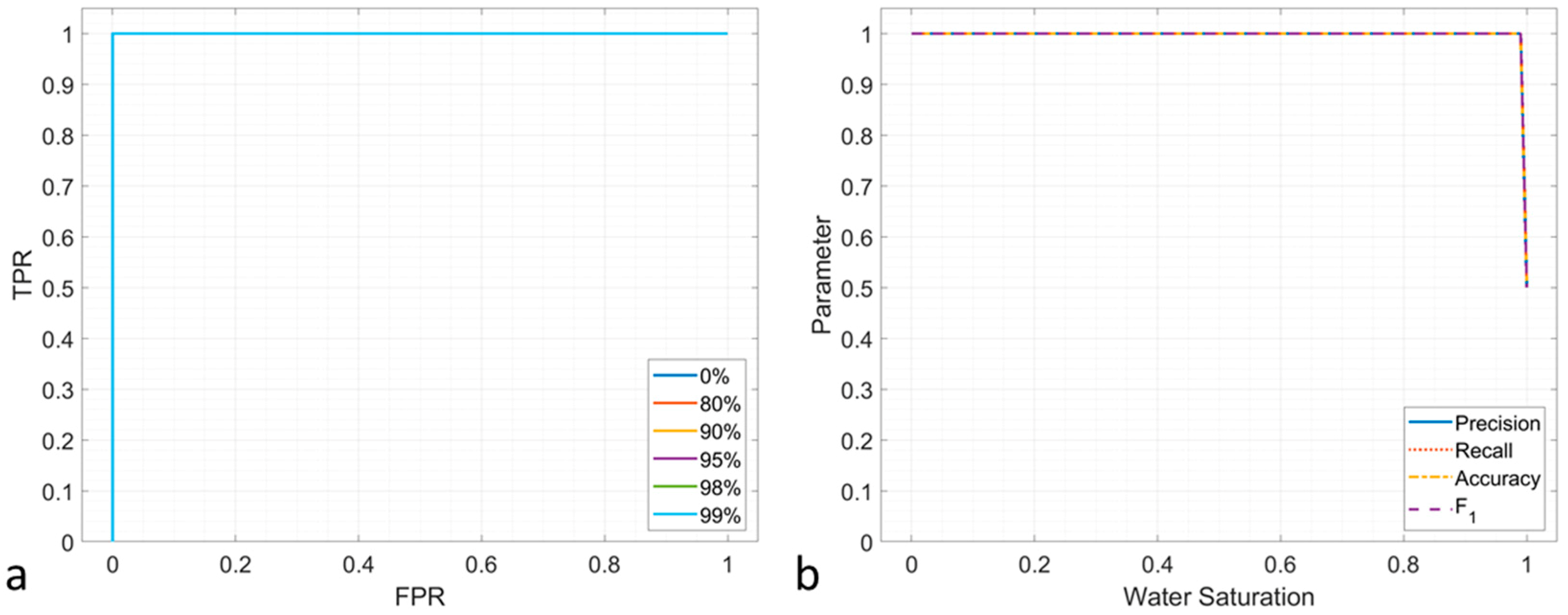
The sensitivity of water saturation in the new fluid factor () is analyzed as shown in Figure 1a. The can distinguish the hydrocarbons accurately when the water saturation is less than 80%. The true prediction ratio (TPR) decreases with increasing water saturation. When the water saturation is 99%, the TPR is approximately 0.75. The performances of the from 0% to 95% of water saturation do not differ significantly. The evaluation metrics of the (the AUC, the precision, the recall, the accuracy and F1) are shown in Figure 1b. These metrics are approximately 0.98 when the water saturation is less than 80%. After that, they start to decrease. Their values are above 0.9, which indicates good performance when the water saturation is less than 90%. When the water saturation is higher than 90%, their values reduce rapidly. The ability of the hydrocarbon prediction is strong even for high water saturation, for example, 95%, which qualifies as good performance in the hydrocarbon prediction field. However, in another aspect, high water saturation is usually not the target in the oil and gas industry.
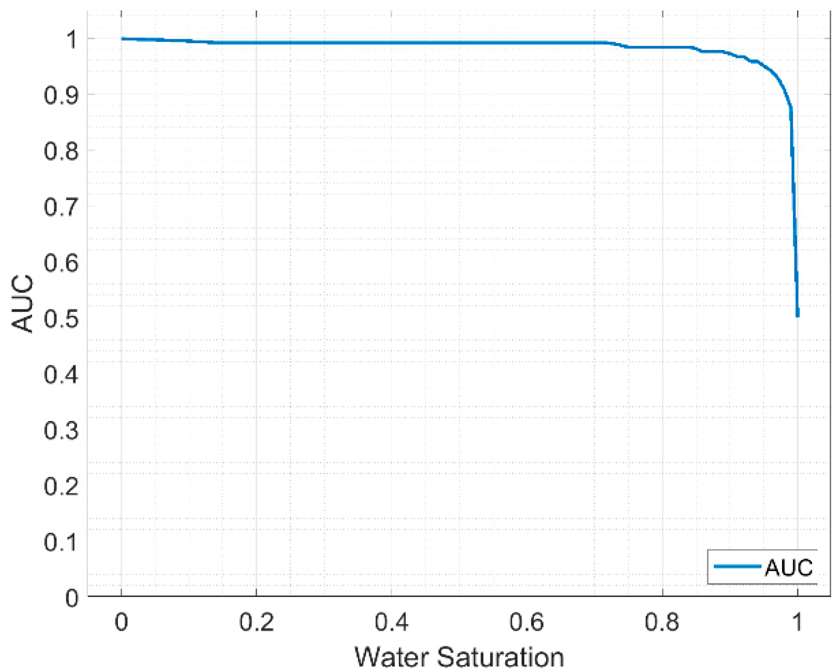
The AUC, which indicates the performance of a binary classifier, is plotted in Figure 2. Its value is higher than 0.95 when the water saturation ranges from 0% to 95%; after that, the AUC decreases rapidly. The performance of the is good when the water saturation of the reservoirs is less than 95%.
3.1.2. Delta K
The ROC of the is plotted in Figure 3a, where the curves for different water saturation conditions overlap entirely. The results show that the performance of is very stable in the different water saturation scenarios. Regardless of the water saturation, can clearly separate the hydrocarbon and brine. Correspondingly, the evaluation metrics of (the precision, the recall, the accuracy and F1) are 1, as shown in Figure 3b.
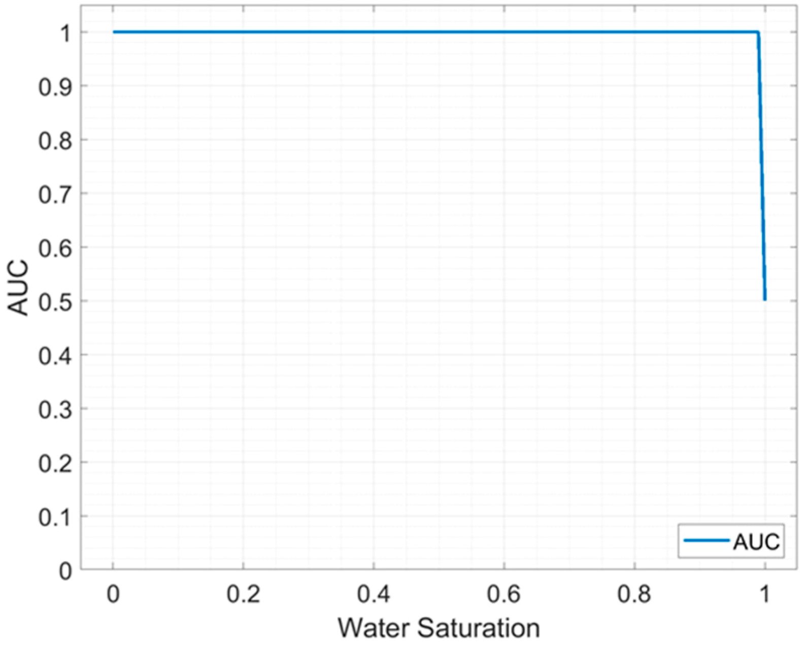
The AUC curve is shown in Figure 4. Its value is 1 when the water saturation ranges from 0 to 99%. The is able to identify the presence of hydrocarbon without the effect of water saturation. It is determined by its definition which is the difference between the in situ pore fluid and the brine. Hence, can detect a hydrocarbon reservoir with a high water saturation.
3.1.3. FFSmith
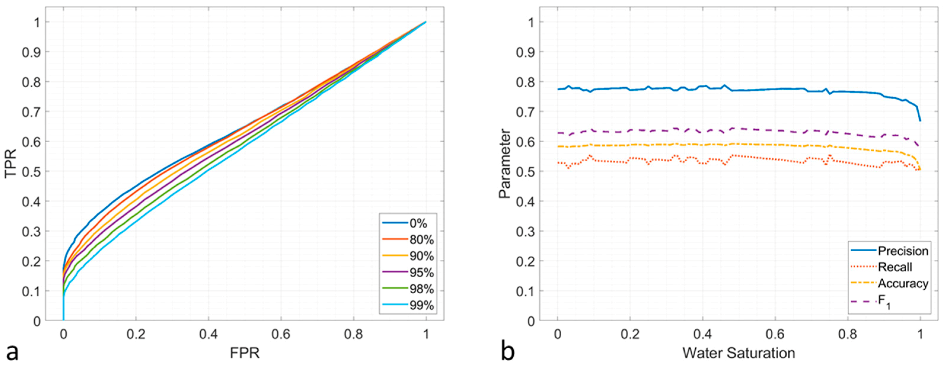
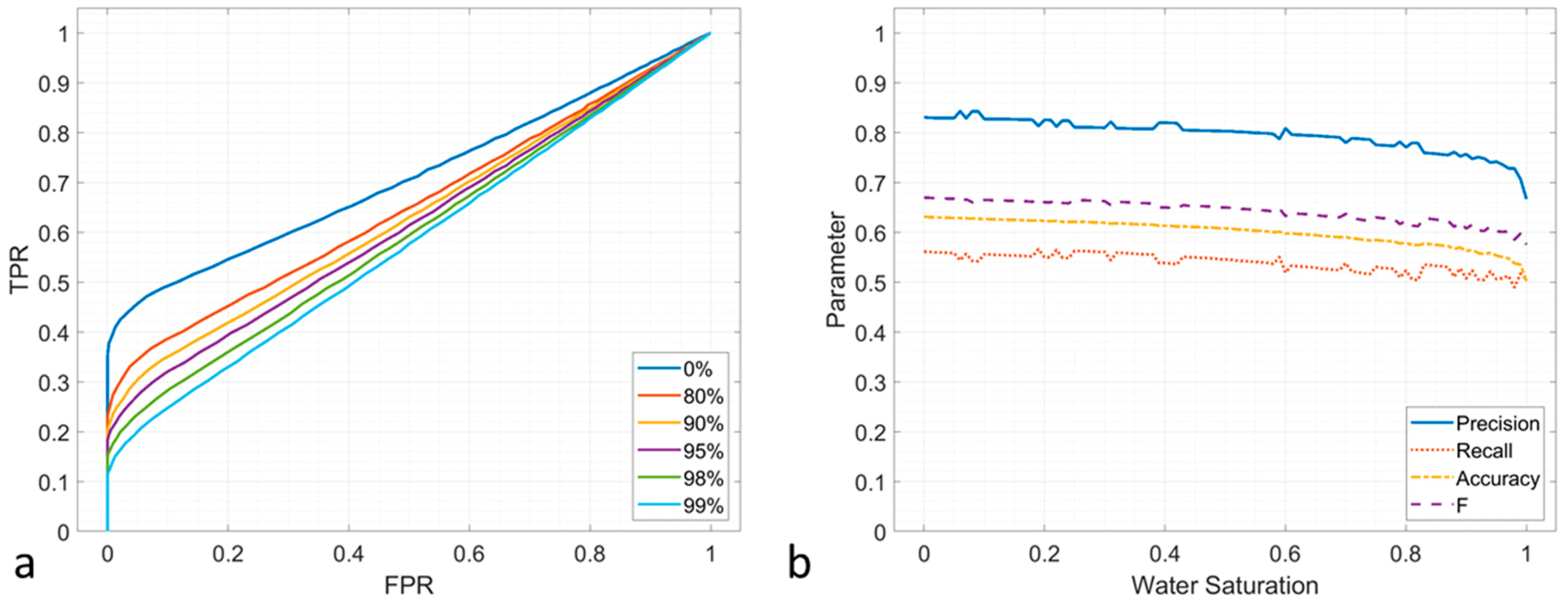
The performances of the traditional fluid factor () are shown in Figure 5. The ROC curves of the in different water saturation scenarios is shown in Figure 5a. The performance is significantly reduced compared with the shown in Figure 1a. The curves for different water saturation plot near the random guess line. The evaluation metrics, which are shown in Figure 5b, indicate the best precision is less than 0.8, while the recall, the accuracy and the F1 have worse performances than the precision.
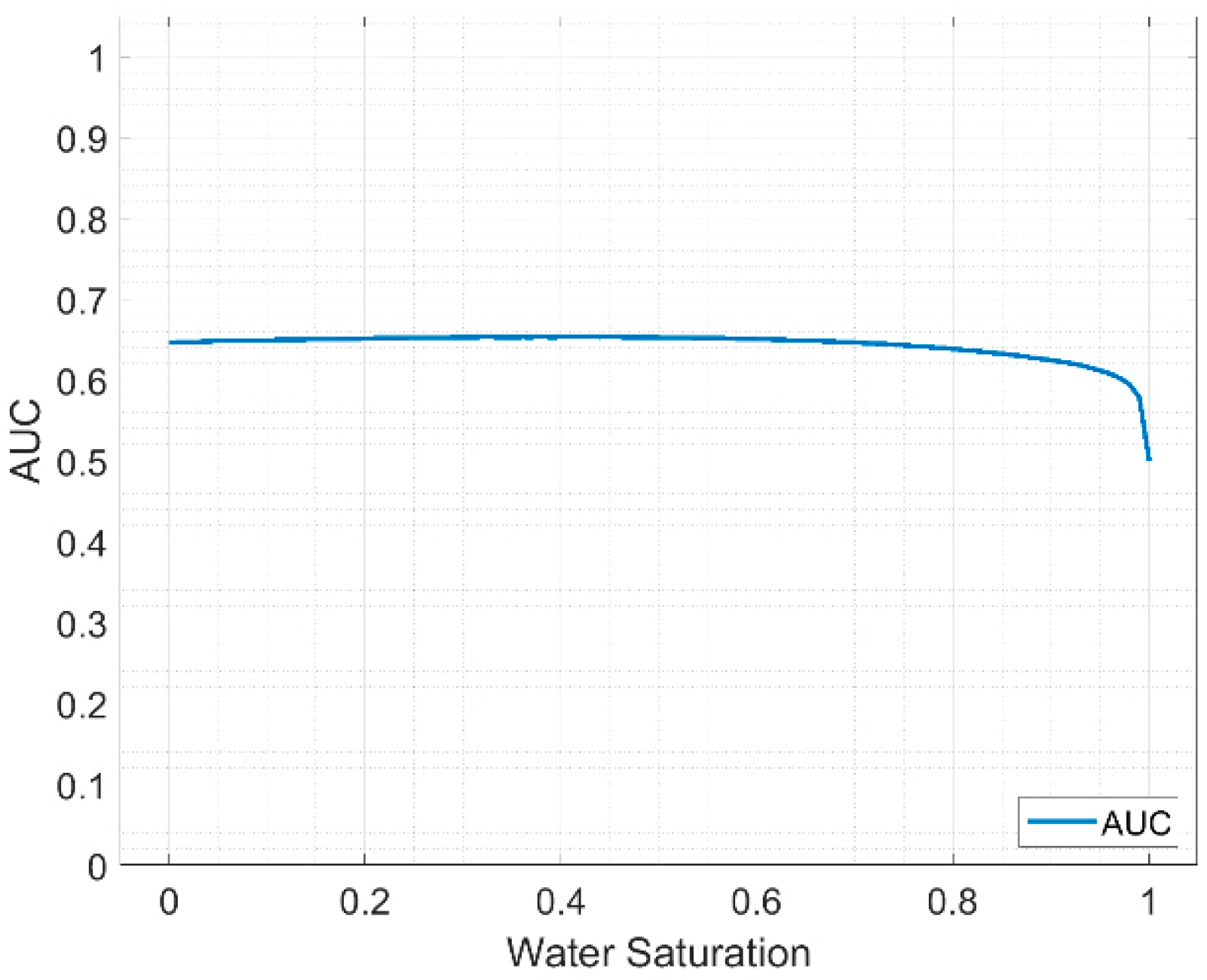
The AUC is plotted in Figure 6. The values are around 0.65 when the water saturation ranges from 0% to 90%. Then the AUC decreases with the increasing water saturation.
3.1.4.
The performances of are shown in Figure 7. The ROC curves of the is shown in Figure 7a. The performance in 0% water saturation scenarios is better than others. The evaluation metrics (Figure 7b) shows the precision decrease gently from 0.85 to 0.75 when the water saturation is changed from 0% to 95%. The values of the recall, the accuracy and the F1 are less than 0.7.
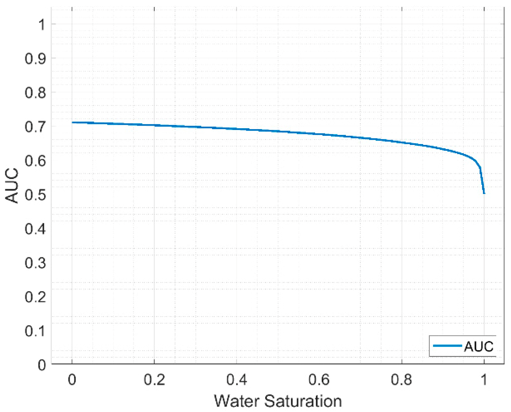
The AUC is plotted in Figure 8. Its value is from 0.7 to 0.6 when the water saturation ranges from 0 to 95%. Then the AUC decreases with the increasing water saturation.
3.2. Uncertainty Analysis under Different Noise Conditions
Noise is unavoidable in the analysis of rock physics. Hence, the uncertainty under noise conditions is an essential ability of the proposed methods. Noise can be ambient or source generated, coherent or random [20]. In a broader sense, noise can be from the uncertainty of the measurement or seismic inversion results. The real data, including well log data, seismic data and inversion data, cannot be noise-free.
Seismic inversion, simultaneous inversion in particular, is a useful tool in quantitative interpretation, although it was not involved in the previous discussion. This technique converts the data from the reflectivity (or interface) domain to the impedance domain, which is more geologically meaningful. Simultaneous inversion can provide information on the P-wave and S-wave velocities and the density in a large area. The accuracy of simultaneous inversion is limited, although it can achieve high accuracy in theory. Its accuracy is dominated by the quality of the input pre-stack seismic data and the well log, the seismic-well tie, and the extracted wavelet together. In a real application, the correlation coefficient between the inverted and real log maybe is not as high as the expectation. Hence, there are errors between the inverted data and the real value. The errors can be regarded as noise when applying the inverted data as the input.
The commonly used unit of noise level is decibel (dB). By definition, the noise level () can be derived by the ratio of energy () or amplitude () between noise and signal as follows:
In this section, the noise levels are set at −20 dB, −10 dB and −7 dB which correspond the energy ratio is 0.01, 0.1 and 0.2. The noise analysis is performed with different water saturation conditions.
3.2.1. FFnew
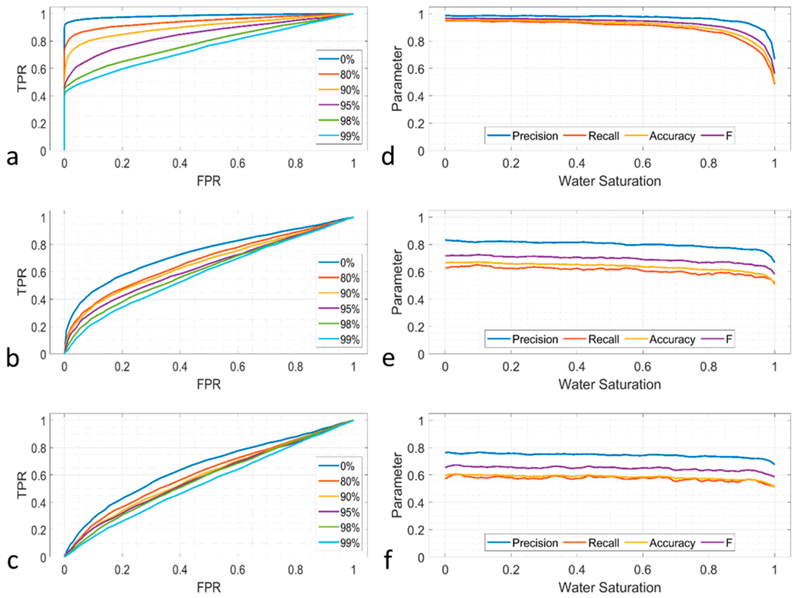
The ROC curves of under different noise levels are shown in Figure 9. The performances of the are high when the noise is relatively low (−20 dB), as shown in Figure 9a. The true prediction ratio decreases when the noise is −20 dB. Furthermore, the performances are worse with increasing noise at −10 dB and −7 dB, as shown in Figure 9b,c. Compared with the −20 dB case, the ROC curves shift towards the random guess line. The ROC curve is close to the random line when the noise reaches −7 dB. which indicates that the performance in a high-noise situation is poor. The evaluation metrics of the are shown in Figure 9d–f. The parameters are above 0.8 when the noise is −20 dB and the water saturation is less than 80%. When the noise is −10 dB, the metrics decrease: the precision is approximately 0.8, whereas the recall, accuracy and F1 are approximately 0.6 to 0.7. When the noise is −7 dB, the parameters reduce continuously. The precision remains at approximately 0.8, whereas the other three parameters are approximately 0.6. Note that the recall is close to 0.5, which indicates that the performance is near that of the random guess.
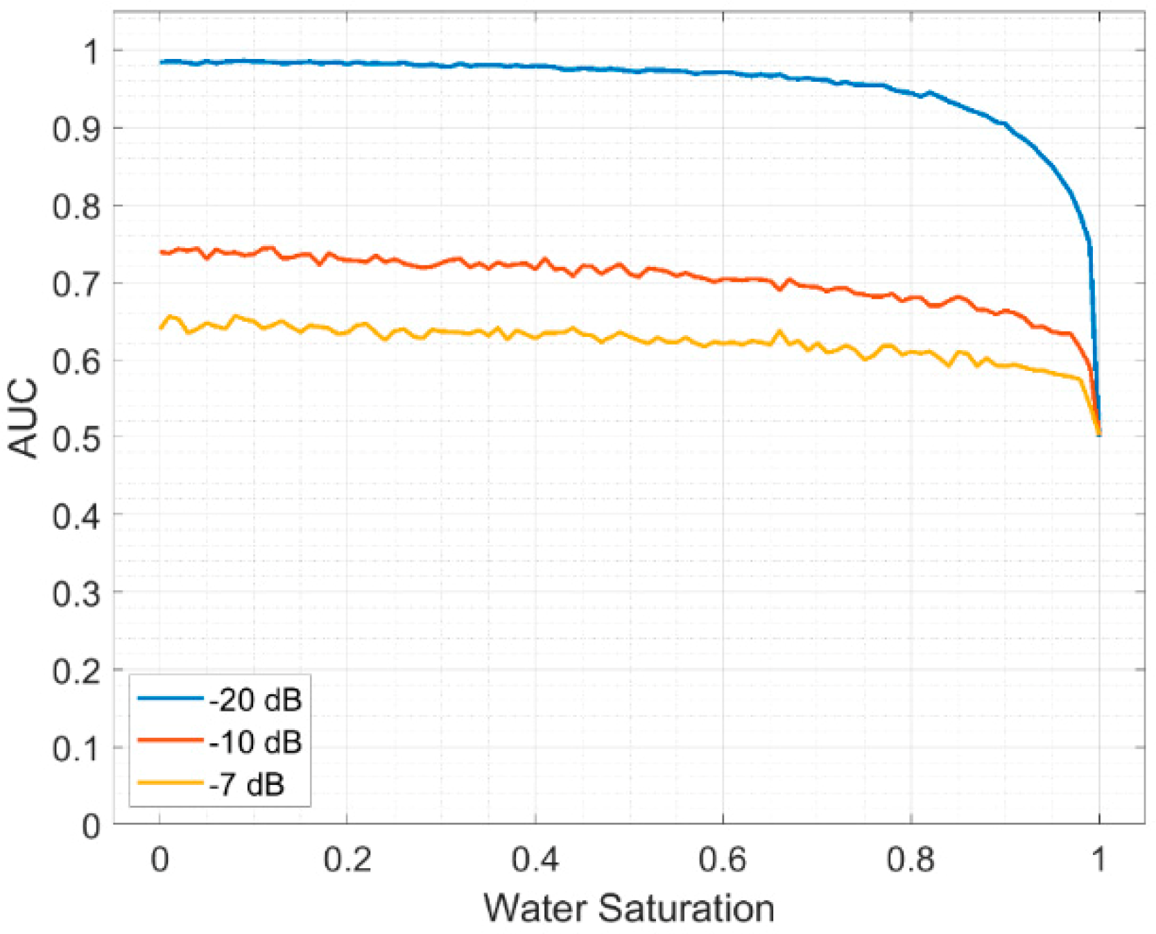
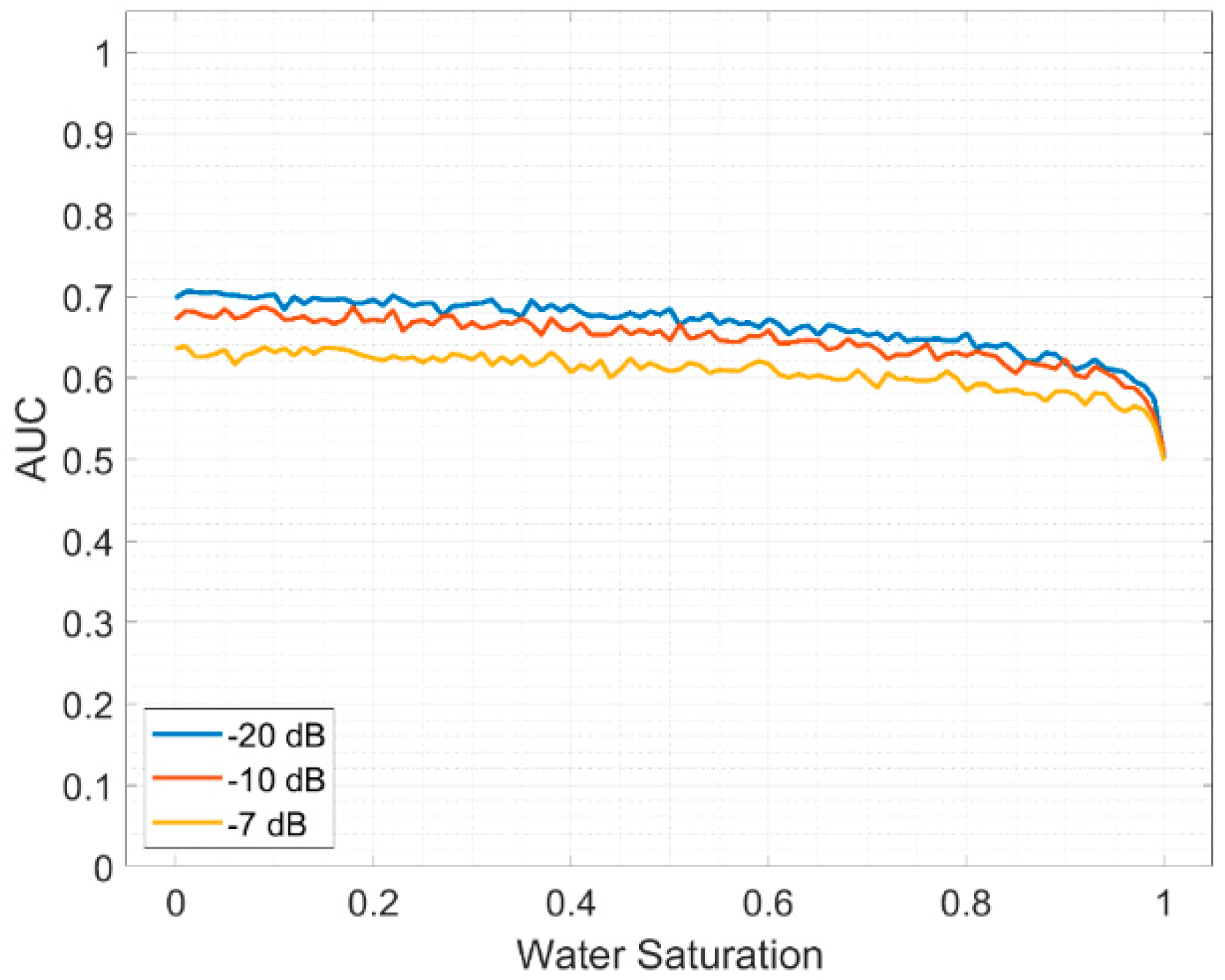
The AUC curves are plotted in Figure 10. The performances in the cases of −20 dB, −10 dB and −7 dB are represented in blue, red and yellow, respectively. The AUC reaches 0.9 when the noise is low. The AUCs decrease with increasing noise. The AUCs are approximately 0.7 and 0.65, respectively, when the noise is −10 dB and −7 dB.
3.2.2. Delta K
The ROC curves of are shown in Figure 11. This parameter performs well when the noise is low (−20 dB), as shown in Figure 11a. The ROC curve is close to the top left corner, which indicates that the prediction reaches a high performance. The TPR is approximately 0.6 even when the water saturation is high (98% and 99%). When the noise is −10 dB, the performance of ROC is worse, as shown in Figure 11b. The lowest TPR is 0.75 when the fluid is saturated hydrocarbon, whereas the TPR values range from 0.4 to 0.6 when the water saturation is higher than 80%. The lowest TPR reduces to 0.6 in the −7 dB noise situation (shown in Figure 11c) when the fluid is saturated hydrocarbon. For cases of high water saturation, the TPR is only 0.2 to 0.4. The evaluation metrics are plotted in Figure 11. The parameters are close to one when the water saturation is low, and the noise is −20 dB, as shown in Figure 11d. The results illustrate that the parameter has good performance when the noise is low. In the scenario where the noise is −10 dB, as shown in Figure 11e, the parameters reduce to different degrees. The precision remains above 0.9, whereas the others range mainly between 0.7 and 0.9. When the noise is −7 dB, the parameters reduce further, as shown in Figure 11f. The precision is between 0.85 and 0.9, whereas the others range from 0.65 to 0.75.
The comparison of the AUC curves in the scenarios where the noise is −20 dB, −10 dB and −7 dB is shown in Figure 12. The performance of decreases with increasing noise. The approximate ranges of the AUC are 0.97 to 1, 0.8 to 0.9 and 0.75 to 0.8 when the noise is −20 dB (blue), −10 dB (red) and −7 dB (yellow), respectively.
3.2.3. FFSmith
The ROC curves of under different noise conditions (−20 dB, −10 dB and −7 dB) are shown in Figure 13a–c, respectively. The shapes of ROC curves are similar, which indicates is less affected by noise. However, the performance of is poor that all the curves gather near the random guess line. The evaluation metrics are plotted in Figure 13d–f. The precision is close to 0.8 when the noise is −20 dB, while the other metrics are less than 0.7 as shown in Figure 13d. The results in −10 dB and −7 dB (Figure 13e and f) are similar to the −20 dB scenario.
The comparison of the AUC curves in the scenarios where the noise is −20 dB, −10 dB and −7 dB is shown in Figure 14. The performance of decreases with increasing noise. The approximate ranges of the AUC are 0.6 to 0.7 when the noise is −20 dB (blue), −10 dB (red) and −7 dB (yellow), respectively.
3.2.4.
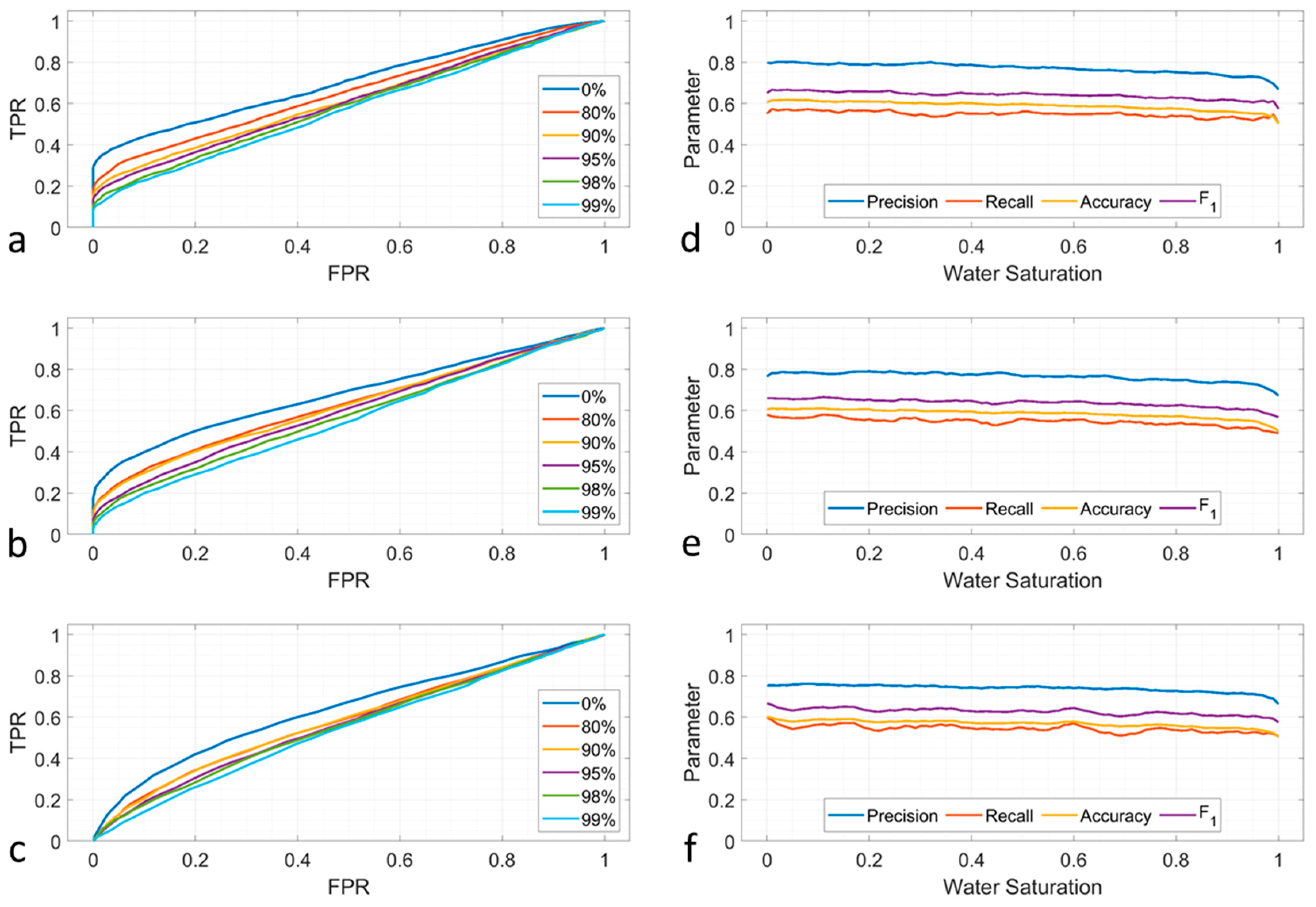
The ROC curves of under different noise conditions (−20 dB, −10 dB and −7 dB) are shown in Figure 15a–c, respectively. The ROC curves shift towards the random guess line with the increasing noise level. The evaluation metrics are given in Figure 15d–f. The precision is close to 0.8 and the other metrics are less than 0.7. The results in −10 dB and −7 dB (Figure 15e,f) are similar to the −20 dB scenario.
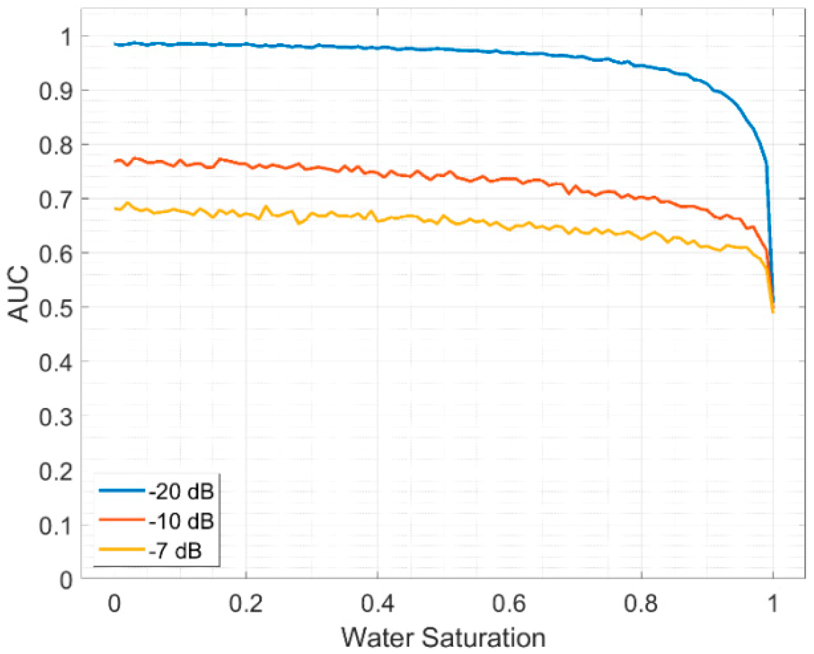
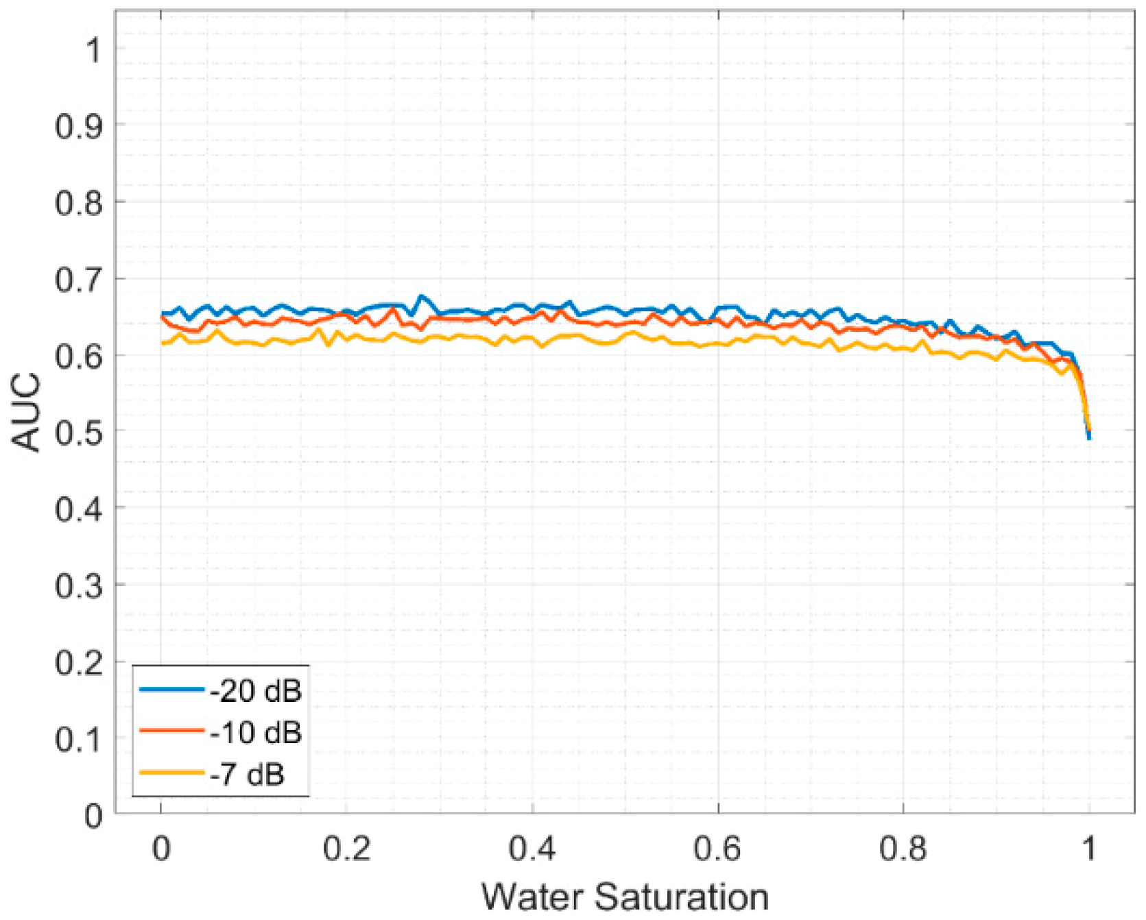
The comparison of the AUC curves in the scenarios where the noise is −20 dB, −10 dB and −7 dB is shown in Figure 16. The performance decreases with increasing noise. The approximate ranges of the AUC are 0.6 to 0.7, 0.58 to 0.68 and 0.55 to 0.65 when the noise is −20 dB (blue), −10 dB (red) and −7 dB (yellow), respectively.
4. Conclusions
Two methods ( and ) have recently been proposed for hydrocarbon prediction. This study analyzes the uncertainty under different-water saturation and noise conditions of these methods, which are not included in the original works [3,11].
Both and keep good performance when water saturation is changed from 0% to 95%. The values of the related metric parameters (precision, recall, accuracy, F-measure and AUC) are greater than 0.9. On the one hand, it illustrates the stability of these methods in hydrocarbon prediction even in a high water saturation scenario. On the other hand, they cannot distinguish low water-saturation reservoirs from high water-saturation reservoirs which is a problem that the industry is facing. A solution of high-water saturation identification is the combination of seismic and controlled-source electromagnetic (CSEM) methods [21].
Noise is another essential factor. In the analysis of this study, the noise levels are set to be −20 dB, −10 dB and −7 dB. The has good performance (the parameters are generally above 0.8) when the level of the noise is low (−20 dB). The AUCs decrease with increasing noise. The AUCs remain above 0.85 when the noise is −10 dB and remain above 0.75 when the noise is −7 dB. The , which is in the interface domain, is more sensitive to noise than the impedance-domain methods. The AUC is approximately 0.7 to 0.75 and 0.6 to 0.65 when the noise is −10 dB and −7 dB, respectively. Although the two attributes have different values for noise sensitivity, the trend is consistent, that is, the stronger the noise, the worse the performance. The attributes in the interface domain are more sensitive to noise. Noise is required to be suppressed to get good results in the application.
In addition, two widely used traditional methods ( and ) are analyzed as comparisons in the reflectivity and impedance domains, respectively. and have much higher precision, recall, accuracy and F1 compared to the traditional methods. and under high noise condition (−7 dB) are still better than the traditional methods, even though and are relatively insensitive to noise.
Author Contributions
Conceptualization, C.L.; methodology, C.L.; code, C.L.; writing—original draft preparation, C.L.; writing—review and editing, C.L.; visualization, C.L.; project administration, D.G. and A.M.A.S.
Funding
This research and the APC were funded by Universiti Teknologi Petronas, grant number 015LC0-075.
Acknowledgments
The authors would like to appreciate Universiti Teknologi PETRONAS (UTP) and Petroliam Nasional Berhad (PETRONAS) for all the resources provided. In addition, many thanks are given to our colleagues in the CSI group.
Conflicts of Interest
The authors declare no conflict of interest.
References
- Smith, G.C.; Gidlow, P.M. Weighted stacking for rock property estimation and detection of gas. Geophys. Prospect. 1987, 35, 993–1014. [Google Scholar] [CrossRef]
- Castagna, J.P.; Batzle, M.L.; Eastwood, R.L. Relationships between compressional-wave and shear-wave velocities in clastic silicate rocks. Geophysics 1985, 50, 571–581. [Google Scholar] [CrossRef]
- Liu, C.; Ghosh, D.P.; Salim, A.M.A.; Chow, W.S. A new fluid factor and its application using a deep learning approach: A new fluid factor and its application. Geophys. Prospect. 2019, 67, 140–149. [Google Scholar] [CrossRef]
- Liu, C.; Ghosh, D. A new seismic attribute for ambiguity reduction in hydrocarbon prediction: Seismic attribute for reducing ambiguity. Geophys. Prospect. 2017, 65, 229–239. [Google Scholar] [CrossRef]
- Ghosh, D.; Sajid, M.; Ibrahim, N.A.; Viratno, B. Seismic attributes add a new dimension to prospect evaluation and geomorphology offshore Malaysia. Lead. Edge 2014, 33, 536–545. [Google Scholar] [CrossRef]
- Ødegaard, E.; Avseth, P. Interpretation of Elastic Inversion Results Using Rock Physics Templates. In Proceedings of the 65th EAGE Conference & Exhibition, Stavanger, Norway, 2–5 June 2003. [Google Scholar]
- Goodway, B.; Chen, T.; Downton, J. Improved AVO Fluid Detection and Lithology Discrimination Using Lamé Petrophysical Parameters; “λρ”, “μρ” & “λ/μ Fluid Stack”, from P and S Inversions; SEG Technical Program Expanded Abstracts 1997; Society of Exploration Geophysicists: New Orleans, LA, USA, 1997; pp. 183–186. [Google Scholar]
- Jing, B.; Ren, J.; Qin, X. Inversion of Reservoir Properties: Quantitative Hydrocarbon Seismic Identification in Tight Carbonate Reservoirs; SEG Technical Program Expanded Abstracts 2015; Society of Exploration Geophysicists: New Orleans, LA, USA, 2015; pp. 2693–2697. [Google Scholar]
- Chopra, S.; Sharma, R.K.; Grech, G.K.; Kjølhamar, B.E. Characterization of shallow high-amplitude seismic anomalies in the Hoop Fault Complex, Barents Sea. Interpretation 2017, 5, 607–622. [Google Scholar] [CrossRef]
- Liu, X.; Chen, Z.; Liu, H.; Zhang, W. Oil Detection Based on Layer Buried-Depth Corrected Elastic Inversion in Deepwater of the Pearl River Basin. In Proceedings of the International Petroleum Technology Conference, Beijing, China, 26–28 March 2019. [Google Scholar]
- Liu, C.; Ghosh, D.; Salim, A.M.A.; Chow, W.S. Fluid Discrimination Using Bulk Modulus and Neural Network. In Proceedings of the International Petroleum Technology Conference, Beijing, China, 26–28 March 2019. [Google Scholar]
- Freitas, C.J. The issue of numerical uncertainty. Appl. Math. Model. 2002, 26, 237–248. [Google Scholar] [CrossRef]
- Kroese, D.P.; Brereton, T.; Taimre, T.; Botev, Z.I. Why the Monte Carlo method is so important today. Wiley Interdiscip. Rev. Comput. Stat. 2014, 6, 386–392. [Google Scholar] [CrossRef]
- Bosch, M.; Cara, L.; Rodrigues, J.; Navarro, A.; Díaz, M. A Monte Carlo approach to the joint estimation of reservoir and elastic parameters from seismic amplitudes. Geophysics 2007, 72, O29–O39. [Google Scholar] [CrossRef]
- Zunino, A.; Mosegaard, K.; Lange, K.; Melnikova, Y.; Hansen, T.M. Monte Carlo reservoir analysis combining seismic reflection data and informed priors. Geophysics 2015, 80, R31–R41. [Google Scholar] [CrossRef]
- Yu, S.; Ma, J.; Osher, S. Monte Carlo data-driven tight frame for seismic data recovery. Geophysics 2016, 81, V327–V340. [Google Scholar] [CrossRef]
- Zhu, D.; Gibson, R. Seismic inversion and uncertainty quantification using transdimensional Markov chain Monte Carlo method. Geophysics 2018, 83, R321–R334. [Google Scholar] [CrossRef]
- Mavko, G.; Mukerji, T.; Dvorkin, J. The Rock Physics Handbook: Tools for Seismic Analysis in Porous Media; Cambridge University Press: Cambridge, UK, 2009. [Google Scholar]
- Fawcett, T. An introduction to ROC analysis. Pattern Recognit. Lett. 2006, 27, 861–874. [Google Scholar] [CrossRef]
- Avseth, P.; Mukerji, T.; Mavko, G. Quantitative Seismic Interpretation: Applying Rock Physics Tools to Reduce Interpretation Risk; Cambridge University Press: Cambridge, UK, 2010. [Google Scholar]
- Ghosh, D.; Halim, M.; Brewer, M.; Viratno, B.; Darman, N. Geophysical issues and challenges in Malay and adjacent basins from an E & P perspective. Lead. Edge 2010, 29, 436–449. [Google Scholar]
Figure 1.
(a) Receiver operating characteristic (ROC) of the new fluid factor (). (b) Evaluation metrics of the vary with water saturation.
Figure 1.
(a) Receiver operating characteristic (ROC) of the new fluid factor (). (b) Evaluation metrics of the vary with water saturation.

Figure 2.
The area under the curve (AUC) of the vary with water saturation.

Figure 3.
(a) ROC of the . (b) Evaluation metrics of the vary with water saturation.

Figure 4.
The AUC of the varies with water saturation.

Figure 5.
The performances of in different water saturation scenarios: (a) ROC curves, (b) evaluation metrics.
Figure 5.
The performances of in different water saturation scenarios: (a) ROC curves, (b) evaluation metrics.

Figure 6.
AUC curve of traditional fluid factor ().

Figure 7.
The performances of in different water saturation scenarios: (a) ROC curves. (b) metric parameters.
Figure 7.
The performances of in different water saturation scenarios: (a) ROC curves. (b) metric parameters.

Figure 8.
AUC curve of .

Figure 9.
The ROCs of the in the different noise scenarios: (a) −20 dB, (b) −10 dB, (c) −7 dB. The metrics of the in the different noise scenarios: (d) −20 dB, (e) −10 dB, (f) −7 dB.
Figure 9.
The ROCs of the in the different noise scenarios: (a) −20 dB, (b) −10 dB, (c) −7 dB. The metrics of the in the different noise scenarios: (d) −20 dB, (e) −10 dB, (f) −7 dB.

Figure 10.
The AUC curves of the in the different noise scenarios: −20 dB, −10 dB and −7 dB, respectively.
Figure 10.
The AUC curves of the in the different noise scenarios: −20 dB, −10 dB and −7 dB, respectively.

Figure 11.
The ROCs of the in the different noise scenarios: (a) −20 dB, (b) −10 dB, (c) −7 dB. The metrics of the in the different noise scenarios: (d) −20 dB, (e) −10 dB, (f) −7 dB.
Figure 11.
The ROCs of the in the different noise scenarios: (a) −20 dB, (b) −10 dB, (c) −7 dB. The metrics of the in the different noise scenarios: (d) −20 dB, (e) −10 dB, (f) −7 dB.

Figure 12.
The AUC curves of the in the different noise scenarios: −20 dB, −10 dB and −7 dB.

Figure 13.
The ROCs of the in the different noise scenarios: (a) −20 dB, (b) −10 dB, (c) −7 dB. The metrics of the in the different noise scenarios: (d) −20 dB, (e) −10 dB, (f) −7 dB.
Figure 13.
The ROCs of the in the different noise scenarios: (a) −20 dB, (b) −10 dB, (c) −7 dB. The metrics of the in the different noise scenarios: (d) −20 dB, (e) −10 dB, (f) −7 dB.

Figure 14.
The AUC curves of the in the different noise scenarios: −20dB, −10 dB and −7 dB.

Figure 15.
The ROCs of the in the different noise scenarios: (a) −20 dB, (b) −10 dB, (c) −7 dB. The metrics of the in the different noise scenarios: (d) −20 dB, (e) −10 dB, (f) −7 dB.
Figure 15.
The ROCs of the in the different noise scenarios: (a) −20 dB, (b) −10 dB, (c) −7 dB. The metrics of the in the different noise scenarios: (d) −20 dB, (e) −10 dB, (f) −7 dB.

Figure 16.
The AUC curves of the in the different noise scenarios: −20dB, −10 dB and −7 dB.


Table 1.
Metrics and definitions.
| Metrics | Definition |
|---|---|
| Precision | |
| Recall | |
| Accuracy | |
| F1 |
© 2019 by the authors. Licensee MDPI, Basel, Switzerland. This article is an open access article distributed under the terms and conditions of the Creative Commons Attribution (CC BY) license (http://creativecommons.org/licenses/by/4.0/).
Share and Cite
MDPI and ACS Style
Liu, C.; Ghosh, D.; Salim, A.M.A. Uncertainty Analysis of Two Methods in Hydrocarbon Prediction under Different Water Saturation and Noise Conditions. Appl. Sci. 2019, 9, 5239. https://0-doi-org.brum.beds.ac.uk/10.3390/app9235239
AMA Style
Liu C, Ghosh D, Salim AMA. Uncertainty Analysis of Two Methods in Hydrocarbon Prediction under Different Water Saturation and Noise Conditions. Applied Sciences. 2019; 9(23):5239. https://0-doi-org.brum.beds.ac.uk/10.3390/app9235239
Chicago/Turabian StyleLiu, Changcheng, Deva Ghosh, and Ahmed Mohamed Ahmed Salim. 2019. "Uncertainty Analysis of Two Methods in Hydrocarbon Prediction under Different Water Saturation and Noise Conditions" Applied Sciences 9, no. 23: 5239. https://0-doi-org.brum.beds.ac.uk/10.3390/app9235239
Note that from the first issue of 2016, this journal uses article numbers instead of page numbers. See further details here.