Forecasting Landslides via Three-Dimensional Discrete Element Modeling: Helong Landslide Case Study


1
College of Construction Engineering, Jilin University, Changchun 130026, China
2
Jilin Sixth Geological Prospecting Engineering Team, Yanji 133401, China
3
Jilin Institute of Geo-Environment Monitoring, Changchun 130021 China
*
Author to whom correspondence should be addressed.
Appl. Sci. 2019, 9(23), 5242; https://0-doi-org.brum.beds.ac.uk/10.3390/app9235242
Submission received: 5 November 2019
/
Revised: 26 November 2019
/
Accepted: 28 November 2019
/
Published: 2 December 2019
(This article belongs to the Section Earth Sciences)
Abstract
:Forecasting the occurrence potential of landslides is important but challenging. We aimed to forecast the failure potential of the Helong landslide, which is temporarily stable but has clearly deformed in recent years. To achieve the goal, we used reconnaissance, remote sensing, drilling, laboratory tests, topographical analysis, and electrical resistivity tomography (ERT). The factor of safety (FOS) of the slope was first calculated using a limit equilibrium method. The results show the FOS of the slope was 1.856 under natural conditions, 1.506 under the earthquake conditions, 1.318 under light rainfall, 0.986 under heavy rainfall, 1.075 under light rainfall and earthquake, and 0.832 under simultaneous heavy rainfall and earthquake. When the FOS is less than 1.35, the slope is considered metastable according to the Technical Code for Building Slope Engineering (GB50330-2013) published by the Chinese Ministry of Housing and Urban-Rural Development. Based on the drilling data and digital elevation data, a three-dimensional discrete element method (DEM) model was used to simulate potential landslides. The simulation was used to examine catastrophic slope failure under heavy rainfall conditions within a range of friction coefficients and the corresponding affected areas were determined. Then, we analyzed a typical run-out process. The dynamic information of the run-out behavior, including velocity, run-out distance, and depth, were obtained, which is useful for decision support and future landslide hazard assessment.
1. Introduction
Landslides are one of the most catastrophic geological disasters, and many landslides occur each year around the world, causing loss of life and property [1,2,3,4,5]. Many slopes are in a metastable state, which means they are currently stable but have a high possibility of failure under the heavy rainfall and some external loads. To mitigate the loss caused by potential landslide hazards, forecasting the areas that would potentially be affected is crucial, but this task is challenging.
Previous studies regarding slope safety were mainly concerned about the stability of the slope, which is reflected in the calculation of the factor of safety (FOS). The calculation of the FOS first depends on the limit equilibrium method (LEM), which is based on statistics [6,7,8]. Then, the finite element method (FEM) is used to calculate the FOS to provide detailed stress and strain information [9,10,11,12,13,14,15]. However, both the LEM and FEM can only be used before failure, and cannot show the post-failure behavior of a sliding mass because LEM cannot calculate strain and displacement, and FEM has limitations when it comes to large-deformation analysis. Thus, assessing the dynamic movement and potential affected area of the post-failure landslide behavior is difficult using these traditional numerical methods.
With the fast development of computational techniques, more numerical methods that can be used to analyze large-deformation problems are being applied to landslide simulations. These methods can be generally divided into two types: continuous and discontinuous methods. The continuous methods describe material behavior using macroscopic constitutive equations of mechanical, hydraulic, and thermal-mechanical behaviors. In addition to FEM, smoothed particle hydrodynamics (SPH) [16,17], the material point method (MPM) [18,19], and computational fluid dynamics (CFD) [20,21,22] are popular continuous methods used in landslide simulation. As for the discontinuous methods, the discrete element method (DEM) [23,24,25,26,27] and discontinuous deformation analysis (DDA) [28,29] are most used. In the discontinuous methods, the material is formed by many discrete blocks, and interaction between the blocks satisfies certain physical laws. The macroscopic behavior of material is reflected by the interaction of the blocks. Although run-out behavior information, such as the run-out distance, velocity, and depth of the source, can be easily acquired from these continuous methods, they cannot simulate mass separation, which is important for the analysis of landslides [24].
In this study, we used a DEM to forecast the failure potential of the Helong landslide, which was found to have a clear deformation in a field investigation in 2018. Before the forecasting work, the stability of the slope was first assessed using LEM. Then, reconnaissance, remote sensing, drilling, laboratory tests, and topographical analysis via electrical resistivity tomography (ERT) were used for the construction of a three-dimensional (3D) DEM model. Information about post-failure behavior was obtained from the simulation, which can be used for disaster prevention and mitigation.
2. Background
2.1. Study Area
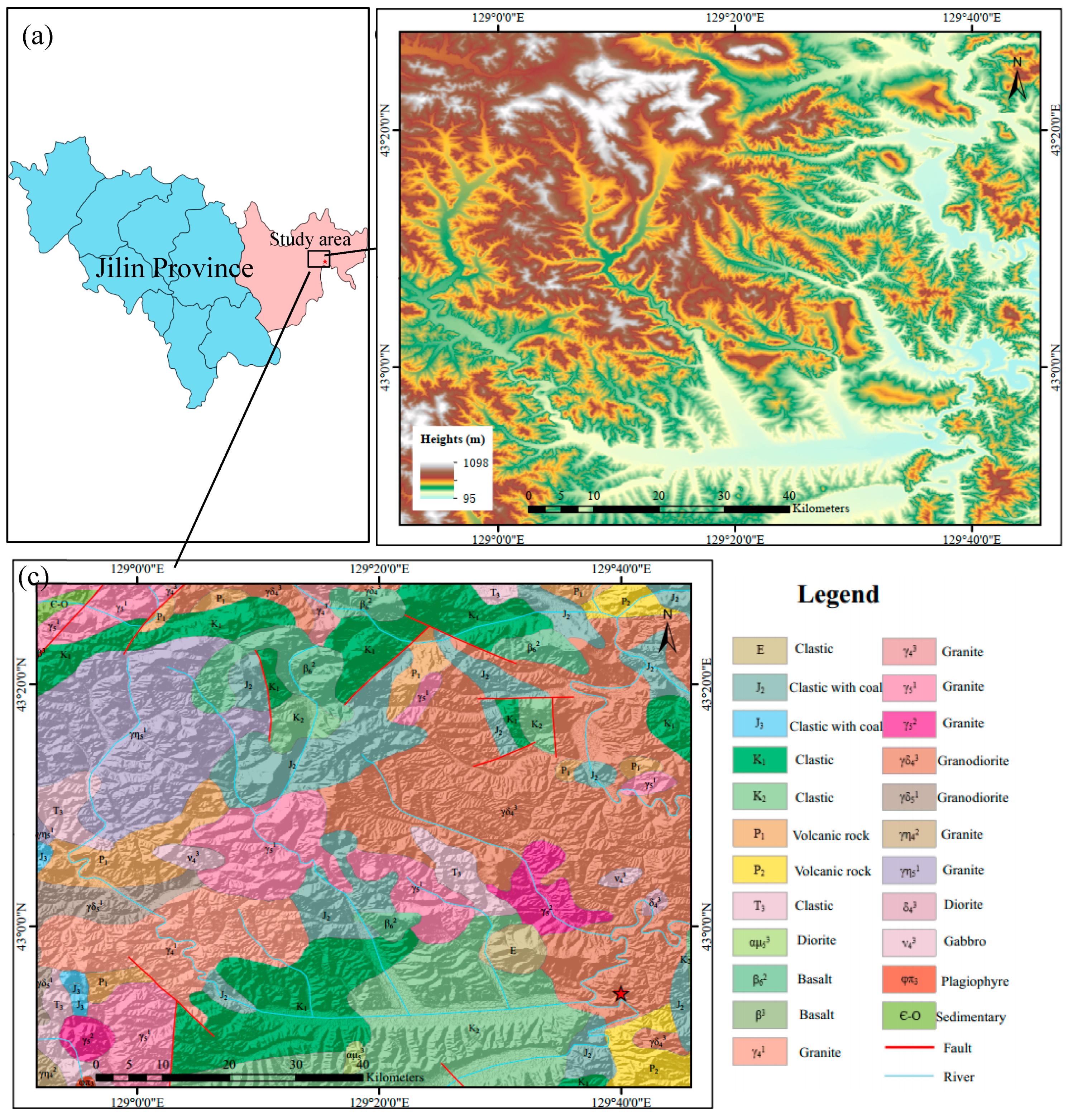
The Helong landslide is located in the southeast of Yanji, Jilin province, China (Figure 1a). The study is a hilly area with an elevation between 59 and 1098 m (Figure 1b). The mountainous ridge is mostly east–west, with slopes between 25° and 30°. Several faults are located in the study area, and the strata around the landslide is mainly composed of granite, sandstone, and mud rock (Figure 1c). Loose material, including eluvium, talus accumulation, and alluvium, is widely distributed on the ground surface.
The study area has a continental monsoon climate with distinct rainy and dry seasons. The average annual rainfall is 521.8 mm, and the wet season occurs from June to August, which receives 60% of the annual precipitation. Concentrated rainfall adversely affects the stability of the slopes, promoting the occurrence of landslides.
2.2. Helong Landslide
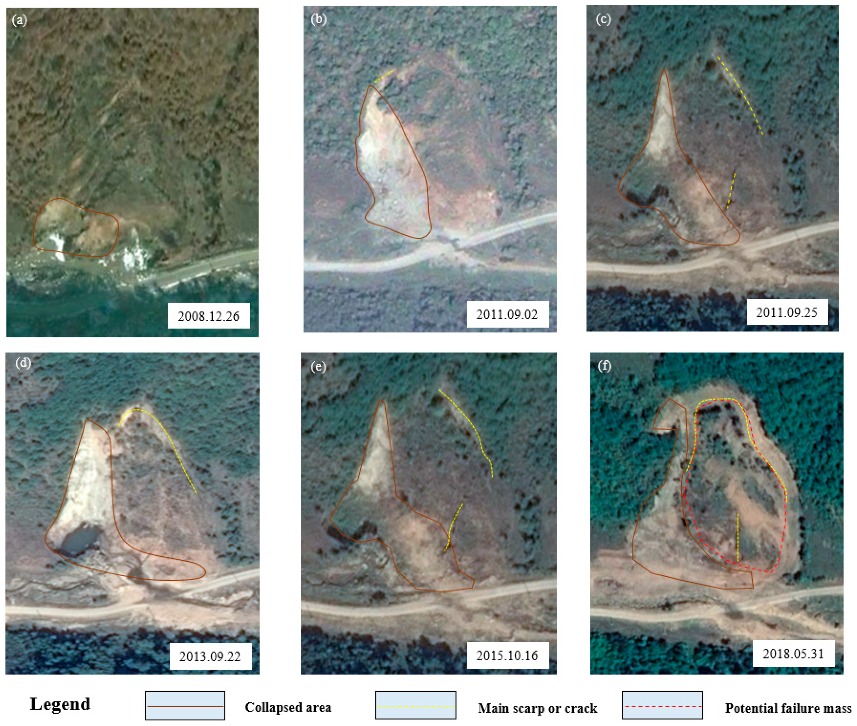
Helong landslide is located on a hill near a road (129°38′12.9″E, 42°54′39.7″N). Part of the slope failed, and a clear deformation of the residual part was observed during a field investigation in 2018. Figure 2 shows the deformation history based on the multi-temporal images obtained from Google Earth. Deformation of the Helong landslide started in December 2008 when a small part of the slope toe collapsed (Figure 2a). Then, a large part of the right slope constantly deformed and failed (Figure 2b,c). After the right part of the slope failed, the left part of the slope started generating cracks and scarps, demonstrating the potential to fail (Figure 2d). In 2018, the slope was still obviously deformed, showing a probability of sliding along the slip surface (Figure 2f).
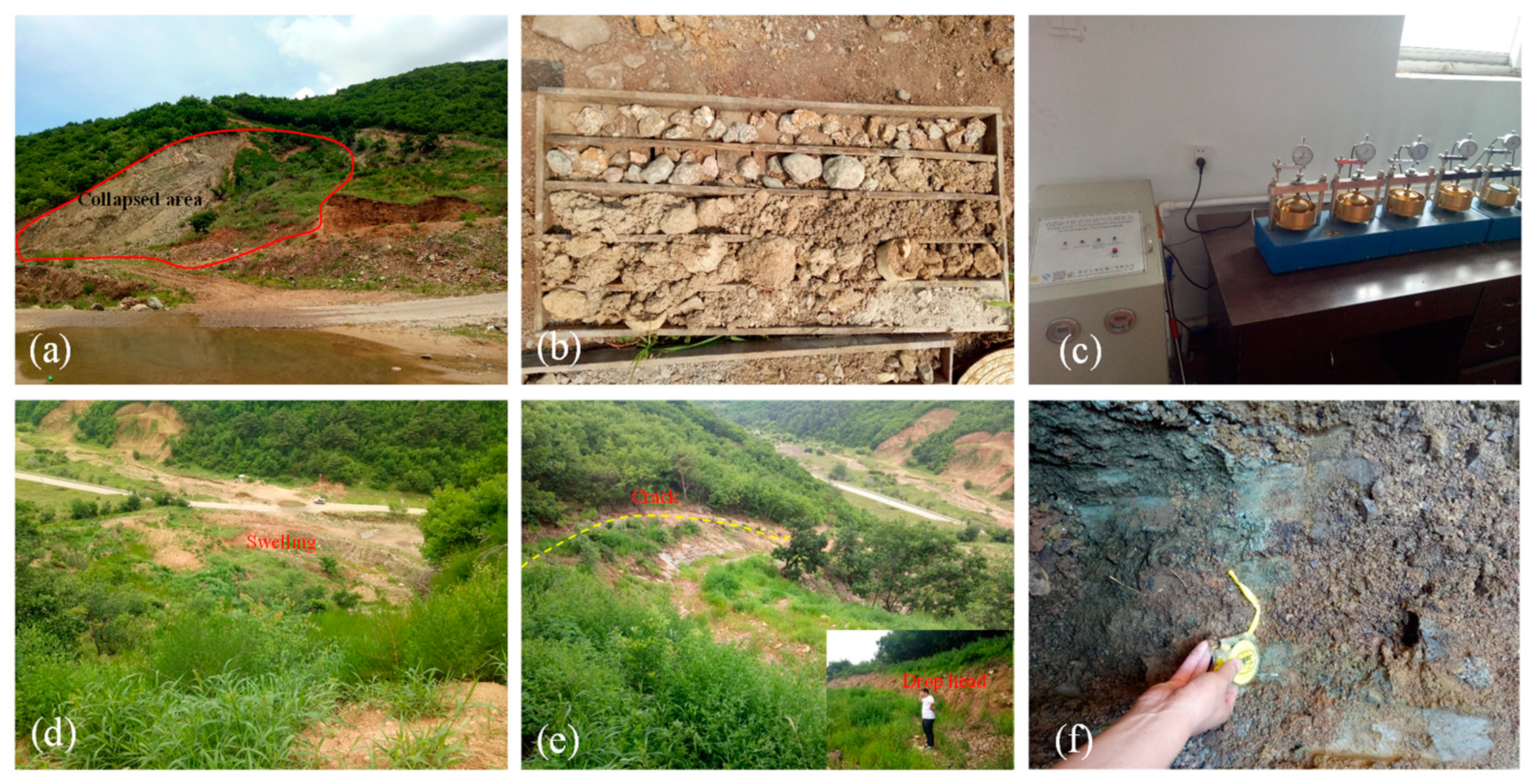
The 3D model of the Helong landslide in 2018 is shown in Figure 3a, with the longitudinal profile of the landslide shown in Figure 3b. On the right side of the potential failure mass, a slide had occurred, leaving a piece of collapsed area (Figure 4a). The source area had obviously deformed, and the potential failure mass was measured as being 150 m long and 110 m wide with an average thickness of 8 m. The composition of the potential failure mass was loose soil aggregate (Figure 4b). Direct shear tests, a consolidation pressure test, and basic physical experiments of soil aggregate under natural and saturated conditions were conducted (Figure 4c). Granite bedrock was below the potential failure mass, and the slip surface was considered to be along the granite bedrock according to the drilling data. The physical and mechanical parameters of relevant materials are shown in Table 1. The front part of the potential failure mass experienced swelling (Figure 4d) and cracks with an obvious drop head were observed at the trailing edge of the landslide (Figure 4e). Because the upper soil aggregate was loose, water could easily be stored (Figure 4f).
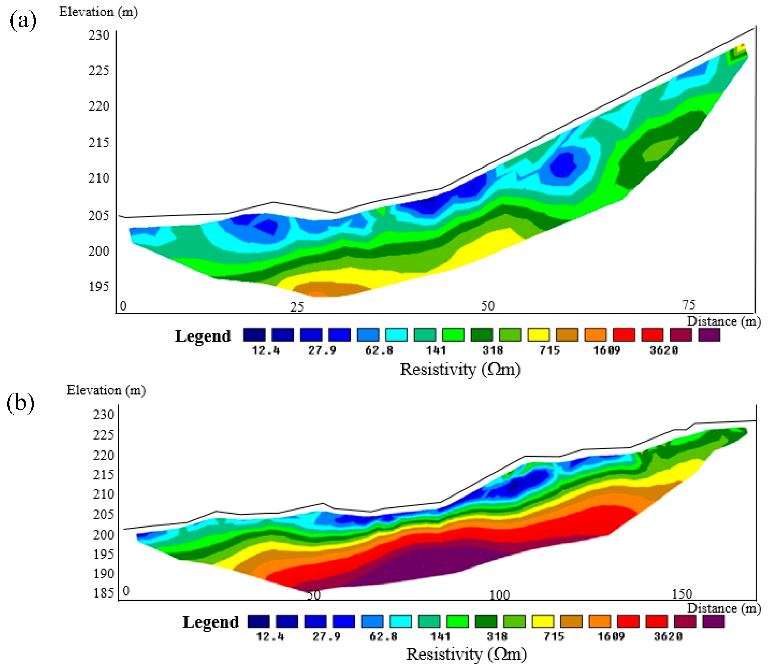
In the investigation, ERT was used to examine the structure and composition of the potential failure zone. ERT is a non-invasive geophysical prospecting method for imaging lateral and vertical variation in subsurface resistivity, and for indirectly mapping geological features [30]. ERT is an electro-exploration method based on the electrical difference in different materials and is used to assess the distribution of geological bodies with different resistivities by utilizing the distribution of electricity within electric fields. Generally, the resistivity of the soil layer is less than 500 Ωm, the resistivity of the rock fracture zone is 500–1700 Ωm, and the intact rock mass is above 1700 Ωm. If the rock and soil have a higher water content, the resistivity significantly decreases. Two ERT profiles, a longitudinal profile and transverse profile, were set, which were acquired with an E60D electric apparatus (Geopen Inc, Beijing, China) with a 3.0 m electrode distance. The results (Figure 5) showed the thickness of the soil ranged from 5 to 10 m, and the resistivity of part of the soil mass was very low, which indicated a high water content in the soil. The results were consistent with the field investigation and drilling data.
The slope was metastable, with a high probability of failing under the influence of water. Considering a road and some buildings were located around the landslide, stability analysis and forecasting the failure potential scale were crucial for mitigating landslide hazards. Thus, we later conducted examinations, including stability analysis based on LEM and failure potential forecasting based on DEM.
3. Methodology
The stability analysis of a slope is based on LEM. LEM is a classical and widely used method for the calculation of the FOS. LEM is used to statically analyze the slope stability. Because the slip surface is generated by shear damage, the FOS is defined as the ratio of the shear strength to the slide force on the slip surface in the LEM, as shown in Equation (1):
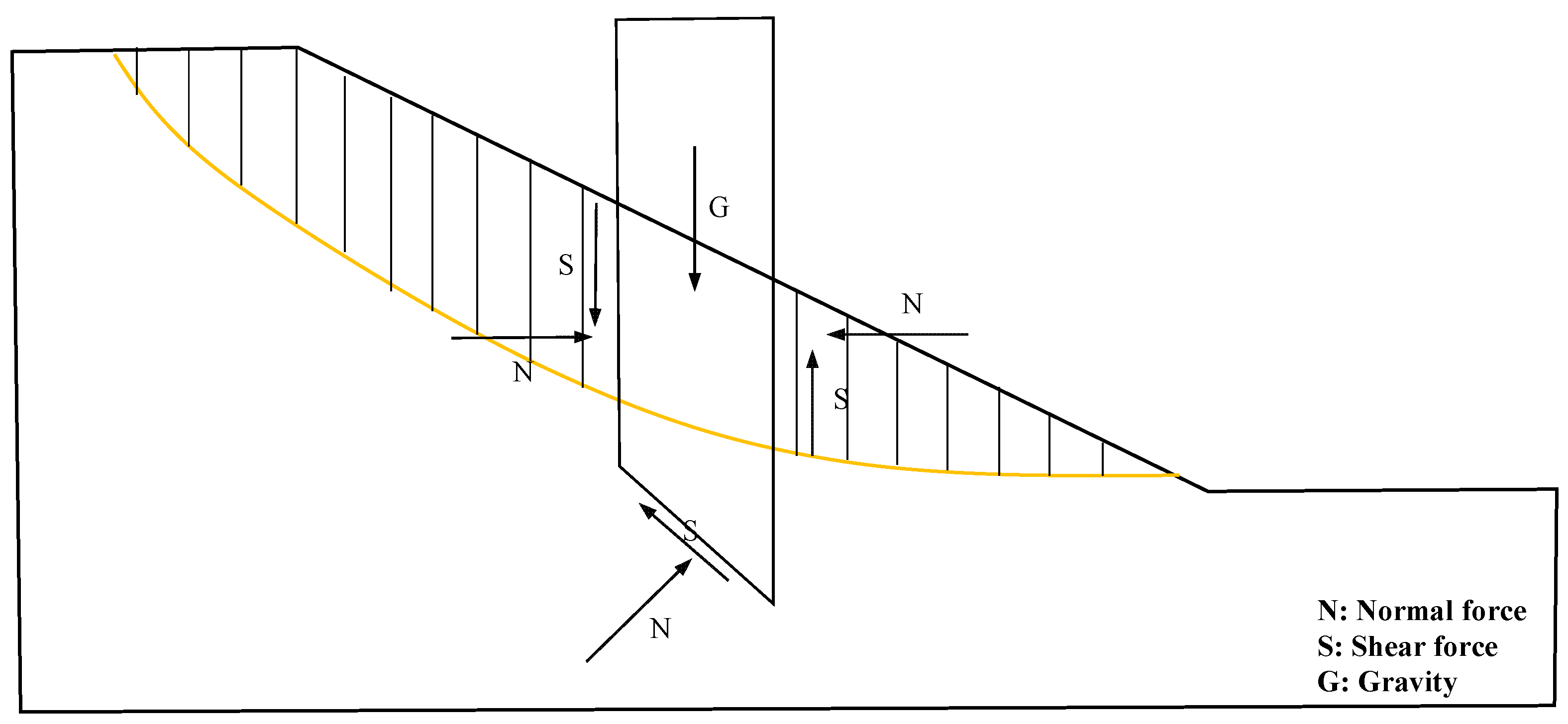
where c is the cohesion of material, is the internal angle of friction of material, σ is the normal compressive stress on slip surface, and τ is the shear strength per unit area on the slip surface. The calculation of forces on the slip surface is based on discrete soil slices (Figure 6). In the LEM, many supposed slip surfaces of the slope are calculated to acquire the FOS, and the most critical slip surface corresponds to the minimum FOS value.
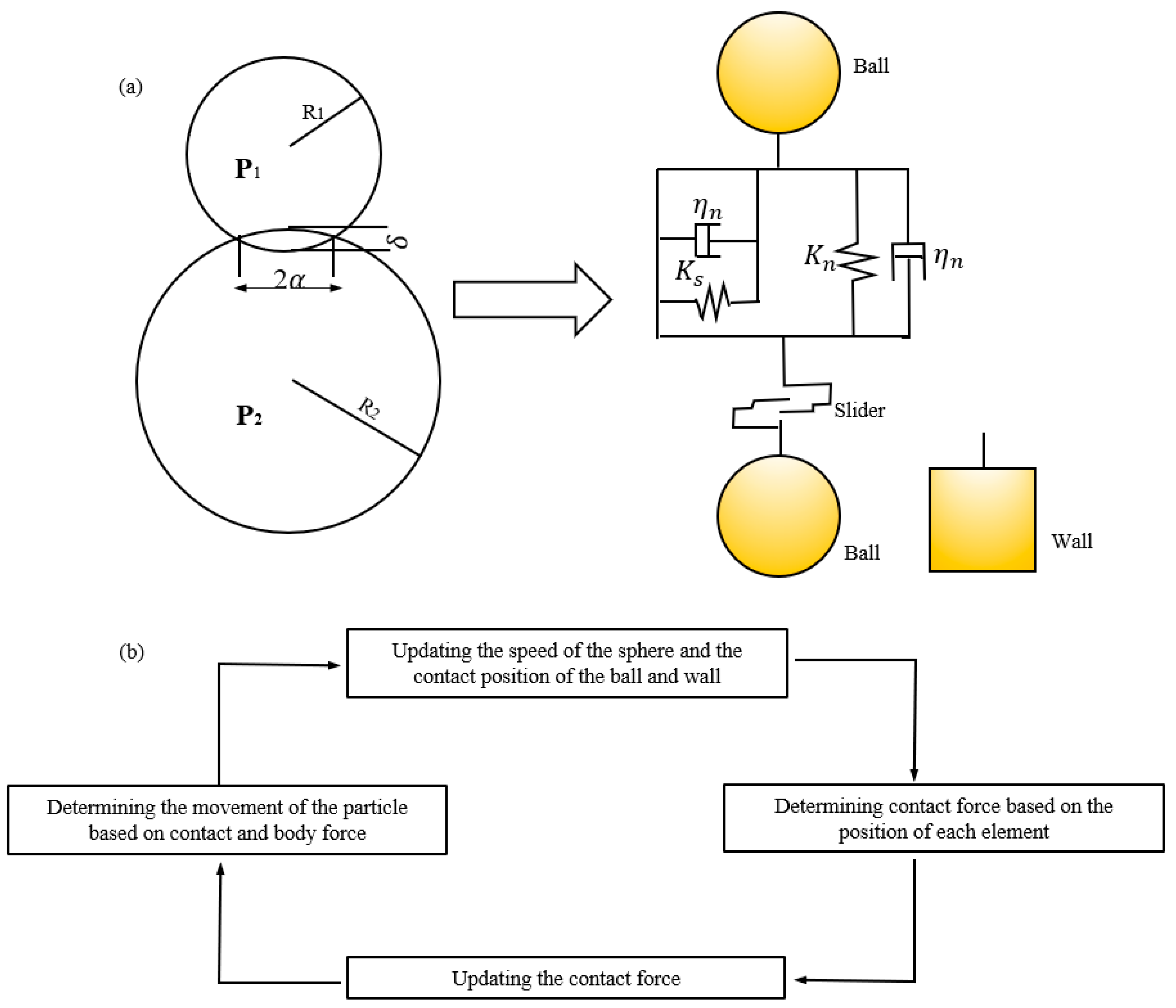
For post-failure analysis, a DEM model was used. DEMs are built based on Newton’s second law and the force–displacement law, shrinking the study scale into a single particle and using the interactions between particles to reflect macroscopic mass behavior. The method includes two kinds of basic elements, a ball and a wall, which are considered as considers the rigid body. Each element is permitted to overlap with adjacent elements to trigger a normal and a tangential force. The inter-particle contacts are usually represented by elastic springs and viscous dampers (Figure 7a). The vibration motion of the particle contact is decomposed into normal and tangential directions. The equation of normal vibrational movement on contact points is expressed in Equation (2), whereas the tangential vibrational movement on contact points is expressed as tangential sliding and rolling movement (Equations (3) and (4)):
where m1,2 is the equivalent mass of particle P1 and P2; I1,2 is the equivalent moment of inertia of the particle; S is the rotation radius; un and us are the normal and tangential relative displacements of the particles, respectively; is the rotation angle of the particle; Fn and Fs are the normal and tangential components of the external force on the particle, respectively; M is the external torque received by the particle; Kn and Ks are the normal and tangential elastic coefficients in the contact model, respectively; and cn and cs are the normal and tangential damping coefficients in the contact model, respectively. For contact points, the magnitude of the force is determined by the magnitude of the overlap. The displacement and velocity are calculated using the original location and force, which are updated according to Newton’s second law of movement in every time step (Figure 7b). The macroscopic physical-mechanical behavior of material is reflected by the microscopic granular interaction using this method.
4. Results and Discussions
4.1. Stability Analysis
To determine the stability of the slope in its current state, we calculated the FOS. The calculation was done using the software Geo-Studio of 2007 version (GEOSLOPE international Ltd., Calgary, Alberta) and Figure 3b was selected as the section to be calculated. Four kinds of situations considering rainfall and an earthquake were set. From the investigation, we believe that the most likely method of slope failure is internal sliding in the upper loose soil, or upper loose soil sliding along the granite bedrock. The type of potential landslide is considered to be translation or rotation. Thus, the Morgenstern–Price method, which fully considers the force balance, as well as the force moment balance and can calculate the slip surface of any shape, was applied to analyze the stability of the landslide [31]. For the rainfall condition, two water lines of different heights were set to represent the groundwater condition during heavy and light rainfalls. The shear strength of soil below the water table was set as the saturated shear strength, whereas the shear strength of the soil above the water table was set as the natural shear strength. According to the Seismic Ground Motion Parameters Zonation Map of China GB18306-2015, the seismic peak ground acceleration of the study area is 0.05 g, and the seismic load was calculated using the pseudo-static method. Other physical and mechanical parameters for calculation were obtained from Table 1.
The results in Figure 8 show that when the slope is under natural conditions, the FOS was 1.856, indicating that the slope was stable without any other external loads. However, when the slope suffered a rainfall or an earthquake, the FOS value decreased sharply. The FOS of the slope was 1.506 under earthquake conditions, 1.318 when the water level was low, and 0.986 when the water level was high. When the slope suffered from a rainfall and an earthquake simultaneously, the FOS was only 1.075 in the low-water-level condition, and 0.832 in the high-water-level condition. The results show that the stability of the slope was sensitive to the level of the water table. According to the Technical Code for Building Slope Engineering (GB50330-2013) published by the Chinese Ministry of Housing and Urban-Rural Development, when the FOS of a slope is less than 1.35, the slope is considered unstable. Thus, forecasting the failure potential of the Helong landslide is vital.
4.2. Post-Failure Analysis
The post-failure behavior of the sliding mass movement was simulated using EDEM 2.7 software (DEM solution Ltd., Edinburgh, Scotland), which was developed by the University of Edinburgh. Before the simulation, a 3D slope model was constructed. We used a DEM with an accuracy of 10 m in 2018 to create the model. Point clouds that contained the terrain position and elevation information were obtained from the digital elevation model, which was then imported into computer automated design (CAD) software Rhino 5.0 (Robert McNeel & Associates Inc, Seattle, Washington). A solid model of the slope that could be used in the numerical simulation was constructed, and the potential sliding mass was extracted based on a field investigation and drilling data.
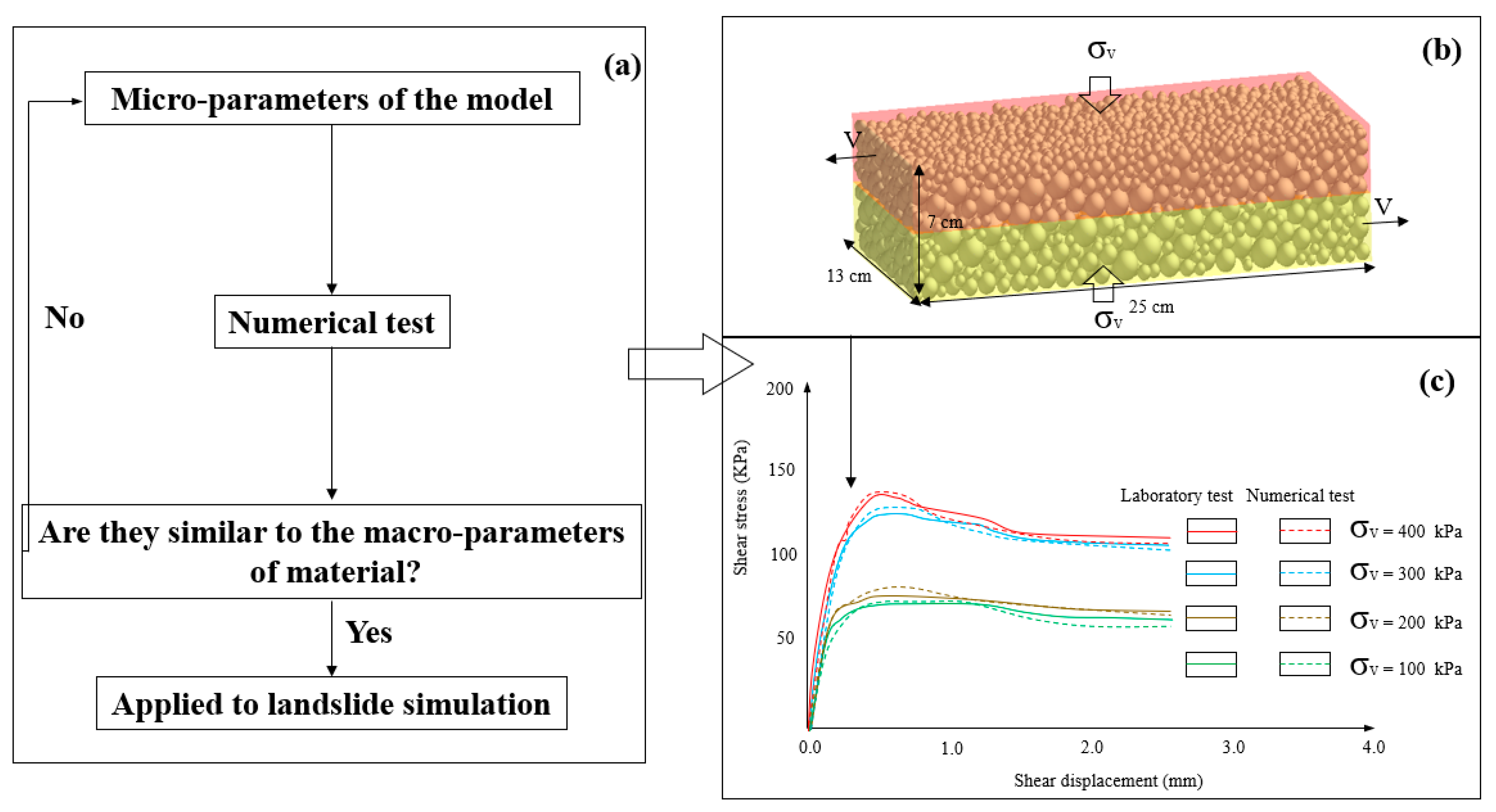
In the DEM simulation, the topography, except the potential sliding mass, was set to be walls to improve the computation efficiency, whereas the sliding mass was set as an aggregate of balls. The bonded particle model (BPM) was used for the potential sliding mass. BPM is conceptually based on bonding together a packed group of spheres to form a breakable body. The bond can transfer force and moment simultaneously, and it ruptures when the tensile stress or shear stress exceeds the tensile or shear strengths. Thus, the BPM is suitable for the simulation of rock and soil behavior [23,24,25]. In the BPM, there are several micro-parameters, including the parameters μ (friction coefficient), E (Young’s modulus), and ν (Poisson’s ratio) between particles; and the bonding parameters (tensile strength of bonding), (shear strength of bonding), (normal bond stiffness of bonding), and (tangential bond stiffness of bonding). The microscopic parameters cannot be measured easily, and a theory is not available to determine the magnitude of the relationship between macroscopic and microscopic parameters. Therefore, in the DEM, parameter calibration experiments are usually performed. A series of numerical simulations are conducted for comparison with laboratory tests. If the outcomes are consistent, then the micro-parameters can be considered appropriate. Soil aggregate parameters were adopted from a numerical shear test, which was calibrated using the real values (Figure 9). The contact parameters between the balls are shown in Table 2. After the 3D slope model was finished (Figure 10), the run-out process was started by reducing the wall friction coefficient below the sliding mass [24].
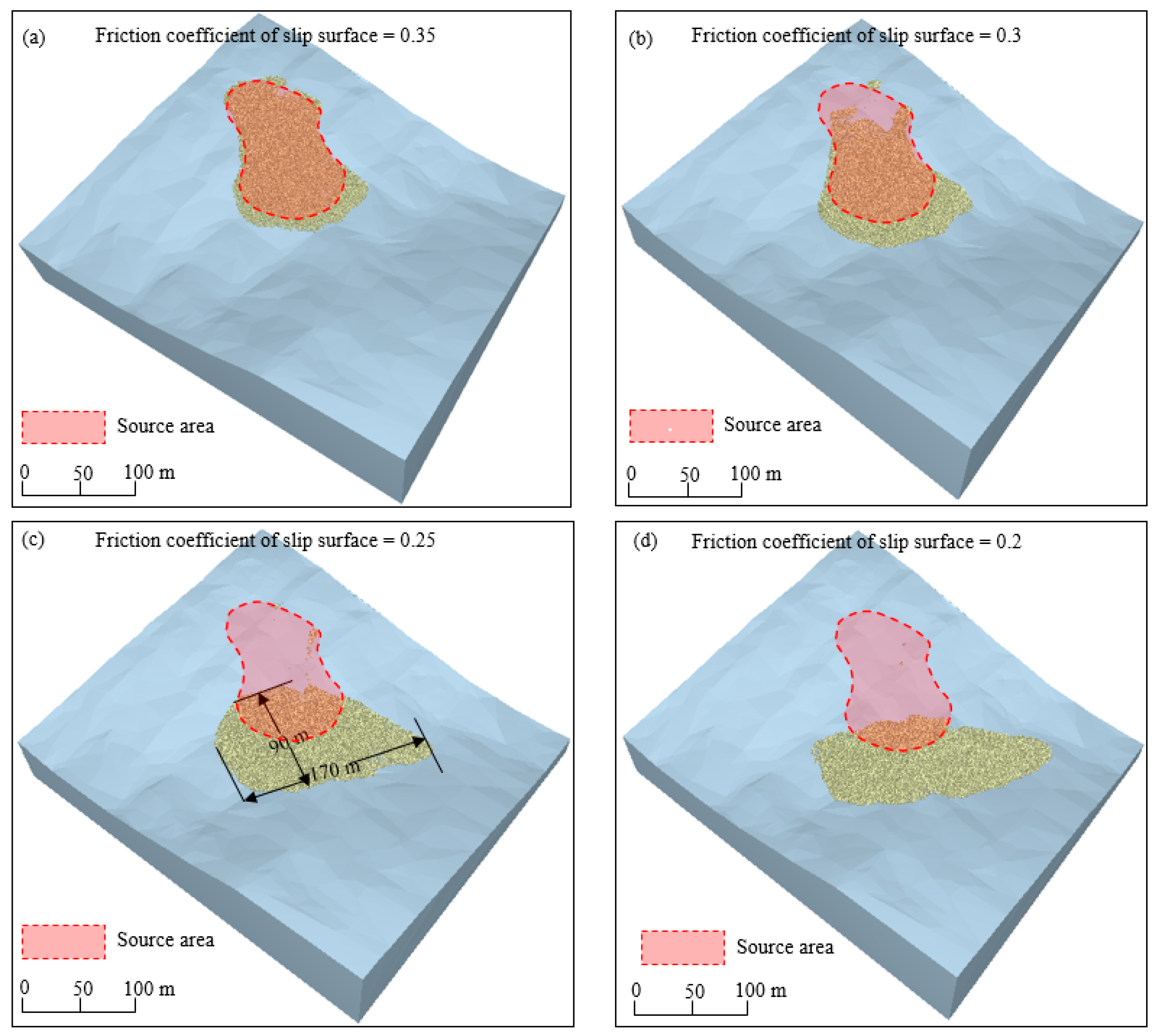
Potential failure of the slope may occur under natural dry conditions or with a rainfall. Therefore, the friction coefficient between the soil and slip surface may differ. According to Table 1, the value of the friction coefficient was 0.36 (20°) under normal conditions and 0.26 (15°) under saturated conditions. Here, we set four groups of friction coefficients for the slip surface: 0.35, 0.30, 0.25, and 0.2. The results showed that with a decreasing friction coefficient, the extent of the potential failure area increased (Figure 11), and the road, as well as some buildings, will be affected when the friction coefficient is lower than 0.3. When the friction coefficient of the slip surface was 0.35, the source basically remained intact, only moving a little downward (Figure 11a). With an increase in humidity, the friction coefficient decreased, and the failure potential area was 170 m long and 90 m wide, with an average depth of 7 m when the source was completely saturated (Figure 11c). The friction coefficient on the slip surface was frequently lower than the internal friction [32,33]; thus, a lower friction coefficient value was used in the simulation (Figure 11d). The result showed that a lower friction coefficient led to a narrower deposit with a larger affected area and less depth.
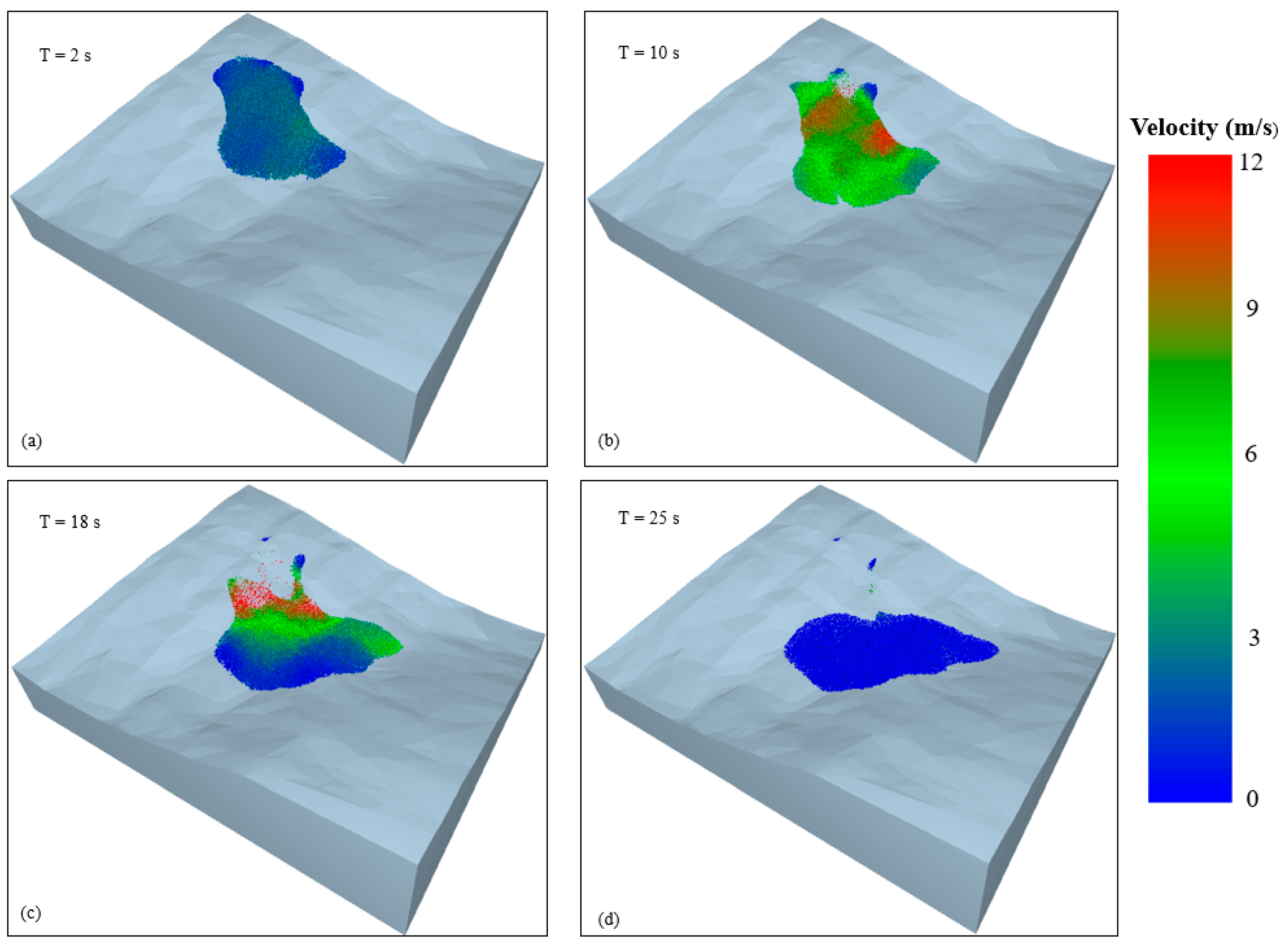
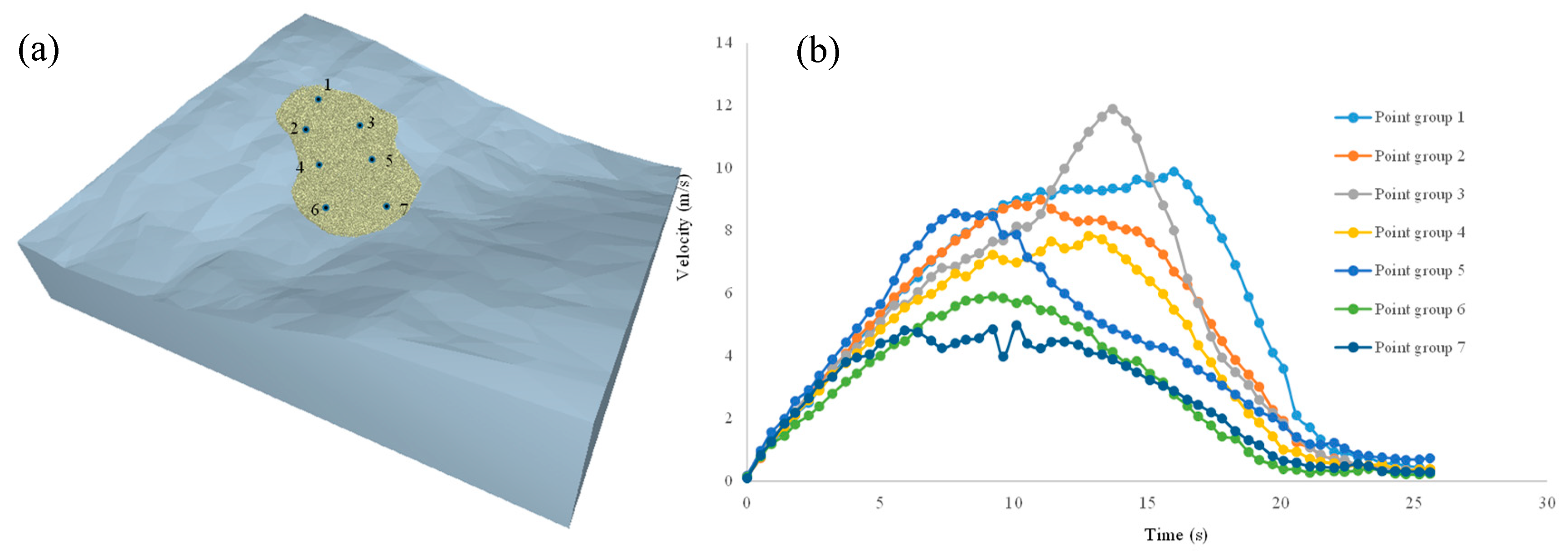
Understanding the dynamic landslide process is important. Here, we selected a friction coefficient of 0.25 as an example for analysis, and the result is shown in Figure 12. The whole potential landslide process lasted 25 s. To obtain detailed information about the run-out process, seven groups of balls were traced and their positions and velocities were recorded in every step (Figure 13a). The sliding mass experienced two stages: acceleration and deceleration (Figure 13b). The period of acceleration ranged from 0 to 15 s, whereas the deceleration occurred from 15 to 25 s. The maximum velocity of the sliding mass was 12 m/s, and the general velocity ranged from 4 to 10 m/s. The velocity of the upper mass was generally higher than the lower mass due to topographical factors. Combined with the swelling phenomenon at the foot of the slope, the potential landslide was a thrust type.
5. Conclusions
In this study, we aimed to forecast the failure potential of the Helong landslide, which was temporarily stable but has a high probability of failure. Remote sensing images from different periods show the process of deformation that has occurred in recent years. Based on a field investigation and laboratory tests, the slope stability was calculated via LEM, and the outcome showed that the slope was metastable and may fail under rainfall or earthquake conditions. Then, we used a 3D DEM to simulate a potential landslide and different conditions were discussed. The results showed a potential failure might affect the surrounding road and buildings. DEM simulated the behavior of landslides well.
Although the findings can be used as an example of the forecasting of the failure potential of landslides, some aspects are worth further exploration and improvement. In the stability analysis under the rainfall condition, we used the natural shear strength for soil above the river table and the saturated shear strength for soil below the water table to calculate the FOS of the slope. The buoyant effect and saturated shear strength could also be considered and incorporated in the calculation of FOS, which is based on statics. However, the effect of rainfall on the slope stability is much more complicated [34,35,36,37], especially for unsaturated soil. Dynamic processes, such as seepage and the variation in pore water pressure from rainfall, affect the slope stability. Determining how to scientifically consider all these factors from rainfall is important but difficult. DEM has some limitations in the simulation of landslides as not all complex landslide mechanisms [38], especially those involving water, such as pore water pressure problems or seepage problems, are considered in the model. Integrating the calculation of FOS and the dynamic post-failure simulation into a model remains an issue. Although DEM can be used to theoretically calculate the FOS of slopes via the strength reduction technique [12,39], the micro-parameters corresponding to the macro-parameters c and φ are too difficult to be determined under different reduction situations. Therefore, future studies should focus on the relationship between micro-parameters and macro-parameters.
Author Contributions
Writing—original draft preparation, W.P.; Project administration, S.S.; Funding acquisition, S.S.; Investigation, C.Y. and J.S.; Resources, C.Y. and J.S.; data curation, C.Y.; Writing—review and editing, Y.H.; Software, Y.B.; Formal analysis, Y.B.
Funding
This research was funded by the National Natural Science Foundation of China (grant no. 41702301), opening fund of the State Key Laboratory of Geohazard Prevention and Geoenvironment Protection (Chengdu University of Technology) (grant no. SKLGP2018K017), and the China Postdoctoral Science Foundation (grant no. 2017M611324).
Acknowledgments
We very thank for all the editors and reviewers who have helped us improve and publish the paper.
Conflicts of Interest
The authors declare no conflict of interest.
References
- Wang, F.; Cheng, Q.; Highland, L.; Miyajima, M.; Wang, H.; Yan, C. Preliminary investigation of some large landslides triggered by the 2008 Wenchuan earthquake, Sichuan Province, China. Landslides 2009, 6, 47–54. [Google Scholar] [CrossRef]
- Ibañez, J.; Hatzor, Y. Rapid sliding and friction degradation: Lessons from the catastrophic Vajont landslide. Eng. Geol. 2018, 244, 96–106. [Google Scholar] [CrossRef]
- García-Delgado, H.; Machuca, S.; Medina, E. Dynamic and geomorphic characterizations of the Mocoa debris flow (March 31, 2017, Putumayo Department, southern Colombia). Landslides 2019, 16, 597–609. [Google Scholar] [CrossRef]
- Tsuguti, H.; Seino, N.; Kawase, H.; Imada, Y.; Nakaegawa, T.; Takayabu, I. Meteorological overview and mesoscale characteristics of the Heavy Rain Event of July 2018 in Japan. Landslides 2019, 16, 363–371. [Google Scholar] [CrossRef]
- Hirota, K.; Konagai, K.; Sassa, K.; Dang, K.; Yoshinaga, Y.; Wakita, E.K. Landslides triggered by the West Japan Heavy Rain of July 2018, and geological and geomorphological features of soaked mountain slopes. Landslides 2019, 16, 189–194. [Google Scholar] [CrossRef]
- Bishop, A.W. The stability of tips and spoil heaps. Q. J. Eng. Geol. Hydrogeol. 1973, 6, 335–376. [Google Scholar] [CrossRef]
- Seed, R.B.; Mitchell, J.K.; Seed, H.B. Kettleman Hills Waste Landfill Slope Failure. II: Stability Analyses. J. Geotech. Geoenviron. Eng. 1990, 116, 669–690. [Google Scholar] [CrossRef]
- Koerner, R.M.; Soong, T.Y. Stability Assessment of Ten Large Landfill Failures. Geo-Denver 2000, 1–38. [Google Scholar] [CrossRef]
- Omraci, K.; Tisot, J.P.; Piguet, J.P. Stability analysis of lateritic waste deposits. Eng. Geol. 2003, 68, 189–199. [Google Scholar] [CrossRef]
- Qu, G.; Hinchberger, S.D.; Lo, K.Y. Case studies of three-dimensional effects on the behaviour of test embankments. Can. Geotech. J. 2009, 46, 1356–1370. [Google Scholar] [CrossRef]
- Rai, R.; Khandelwal, M.; Jaiswal, A. Application of geogrids in waste dump stability: A numerical modeling approach. Environ. Earth Sci. 2012, 66, 1459–1465. [Google Scholar] [CrossRef]
- Bao, Y.; Han, X.; Chen, J.; Zhang, W.; Zhan, J.; Sun, X.; Chen, M. Numerical assessment of failure potential of a large mine waste dump in Panzhihua City, China. Eng. Geol. 2019, 253, 171–183. [Google Scholar] [CrossRef]
- Bao, Y.; Chen, J.; Sun, X.; Han, X.; Song, S. Stability analysis of large waste dumps considering cracks and earthquake via a three-dimension numerical modeling: A case study of Zhujiabaobao waste dump. Q. J. Eng. Geol. Hydrogeol. 2019. [Google Scholar] [CrossRef]
- Li, Y.; Qian, C.; Fu, Z.; Li, Z. On Two Approaches to Slope Stability Reliability Assessments Using the Random Finite Element Method. Appl. Sci. 2019, 9, 4421. [Google Scholar] [CrossRef]
- Dong, L.; Yang, Y.; Qian, B.; Tan, Y.; Sun, H.; Xu, N. Deformation Analysis of Large-Scale Rock Slopes Considering the Effect of Microseismic Events. Appl. Sci. 2019, 9, 3409. [Google Scholar] [CrossRef]
- Li, L.; Wang, Y.; Zhang, L.; Choi, C.; Ng, C.W.W. Evaluation of Critical Slip Surface in Limit Equilibrium Analysis of Slope Stability by Smoothed Particle Hydrodynamics. Int. J. Geomech. 2019, 19, 5. [Google Scholar] [CrossRef]
- Ray, R.; Deb, K.; Shaw, A. Pseudo-Spring smoothed particle hydrodynamics (SPH) based computational model for slope failure. Eng. Anal. Bound. Elem. 2019, 101, 139–148. [Google Scholar] [CrossRef]
- Liu, X.; Wang, Y.; Li, D. Investigation of slope failure mode evolution during large deformation in spatially variable soils by random limit equilibrium and material point methods. Comput. Geotech. 2019, 111, 301–312. [Google Scholar] [CrossRef]
- Conte, E.; Pugliese, L.; Troncone, A. Post-failure stage simulation of a landslide using the material point method. Eng. Geol. 2019, 253, 149–159. [Google Scholar] [CrossRef]
- Han, X.; Chen, J.; Xu, P.; Niu, C.; Zhan, J. Runout analysis of a potential debris flow in the dongwopu gully based on a well-balanced numerical model over complex topography. Bull. Eng. Geol. Environ. 2018, 77, 679–689. [Google Scholar] [CrossRef]
- Han, X.; Chen, J.; Xu, P.; Zhan, J. A well-balanced numerical scheme for debris flow run-out prediction in Xiaojia Gully considering different hydrological designs. Landslides 2017, 14, 2105–2114. [Google Scholar] [CrossRef]
- Bao, Y.; Sun, X.; Chen, J.; Zhang, W.; Han, X.; Zhan, J. Stability assessment and dynamic analysis of a large iron mine waste dump in Panzhihua, Sichuan, China. Environ. Earth Sci. 2019, 78, 48. [Google Scholar] [CrossRef]
- Zhou, J.; Huang, K.; Shi, C.; Hao, M. Discrete element modeling of the mass movement and loose material supplying the gully process of a debris avalanche in the Bayi Gully, Southwest China. J. Asian Earth Sci. 2015, 99, 95–111. [Google Scholar] [CrossRef]
- Lin, C.; Lin, M. Evolution of the large landslide induced by Typhoon Morakot: A case study in the Butangbunasi River, southern Taiwan using the discrete element method. Eng. Geol. 2015, 197, 172–187. [Google Scholar] [CrossRef]
- Lo, C.; Huang, W.; Lin, M. Earthquake-induced deep-seated landslide and landscape evolution process at Hungtsaiping, Nantou County, Taiwan. Environ. Earth Sci. 2016, 75, 645. [Google Scholar] [CrossRef]
- Bao, Y.; Zhai, S.; Chen, J.; Xu, P.; Sun, X.; Zhan, J.; Zhang, W.; Zhou, X. The evolution of the Samaoding paleolandslide river blocking event at the upstream reaches of the Jinsha River, Tibetan Plateau. Geomorphology 2019, 351, 106970. [Google Scholar] [CrossRef]
- Chen, X.; Wang, H. Slope Failure of Noncohesive Media Modelled with the Combined Finite–Discrete Element Method. Appl. Sci. 2019, 9, 579. [Google Scholar] [CrossRef]
- Koyama, T.; Nishiyama, S.; Yang, M.; Ohnishi, Y. Modeling the interaction between fluid flow and particle movement with discontinuous deformation analysis (DDA) method. Int. J. Numer. Anal. Methods Geomech. 2014, 35, 1–20. [Google Scholar] [CrossRef]
- Chen, K.T.; Wu, J.H. Simulating the failure process of the xinmo landslide using discontinuous deformation analysis. Eng. Geol. 2018, 239, 261–281. [Google Scholar] [CrossRef]
- Zhan, J.; Wang, Q.; Zhang, W.; Shangguan, Y.; Song, S.; Chen, J. Soil-engineering properties and failure mechanisms of shallow landslides in soft-rock materials. Catena 2019, 181, 104093. [Google Scholar] [CrossRef]
- Yin, Y.P.; Li, B.; Wang, W.P.; Zhan, L.T.; Xue, Q.; Gao, Y.; Zhang, N.; Chen, H.Q.; Liu, T.K.; Li, A.G. Mechanism of the december catastrophic landslide at the shenzhen landfill and controlling geotechnical risks of urbanization. Engineering 2016, 2, 230–249. [Google Scholar] [CrossRef] [Green Version]
- Aaron, J.; Hungr, O. Dynamic analysis of an extraordinarily mobile rock avalanche in the Northwest Territories, Canada. Can. Geotech. J. 2016, 53, 899–908. [Google Scholar] [CrossRef]
- Aaron, J.; McDougall, S. Rock avalanche mobility: The role of path material. Eng. Geol. 2019, 257, 105126. [Google Scholar] [CrossRef]
- Acharya, K.P.; Bhandary, N.P.; Dahal, R.K.; Yatabe, R. Seepage and slope stability modelling of rainfall-induced slope failures in topographic hollows. Geomat. Nat. Hazards Risk 2016, 7, 721–746. [Google Scholar] [CrossRef]
- Lee, D.; Lai, M.; Wu, J.; Chi, Y.; Ko, W.; Lee, B. Slope management criteria for Alishan Highway based on database of heavy rainfall-induced slope failures. Eng. Geol. 2013, 162, 97–107. [Google Scholar] [CrossRef]
- Qin, Z.; Fu, H.; Chen, X. A study on altered granite meso-damage mechanisms due to water invasion-water loss cycles. Environ. Earth Sci. 2019, 78, 428. [Google Scholar] [CrossRef]
- Wang, J.; Li, S.; Li, L.; Lin, P.; Xu, Z.; Gao, C. Attribute recognition model for risk assessment of water inrush. Bull. Eng. Geol. Environ. 2019, 78, 1067–1071. [Google Scholar] [CrossRef]
- Lu, C.; Tang, C.; Chan, Y.; Hu, J.; Chi, C. Forecasting landslide hazard by the 3D discrete element method: A case study of the unstable slope in the Lushan hot spring district, central Taiwan. Eng. Geol. 2014, 183, 14–30. [Google Scholar] [CrossRef]
- Matsui, T.; San, K.C. Finite element slope stability analysis by shear strength reduction technique. Soils Found. 1992, 32, 59–70. [Google Scholar] [CrossRef] [Green Version]
Figure 1.
The study area: (a) location, (b) topographic, and (c) geological maps.

Figure 2.
Visual interpretation of historical deformation of the rockslide from Google Earth images (the date is shown using the YYYY.MM.DD format). (a) 2008.12.26, (b) 2011.09.02, (c) 2011.09.25, (d) 2013.09.22, (e) 2015.10.16, (f) 2018.05.31.
Figure 2.
Visual interpretation of historical deformation of the rockslide from Google Earth images (the date is shown using the YYYY.MM.DD format). (a) 2008.12.26, (b) 2011.09.02, (c) 2011.09.25, (d) 2013.09.22, (e) 2015.10.16, (f) 2018.05.31.

Figure 3.
Overview of Helong landslide: (a) three-dimensional (3D) scene model and (b) AA’ profile of Helong landslide in Figure 3a (ERT in the Figure 3a denotes electrical resistivity tomography).

Figure 4.
Photographs of the Helong landslide in April 2018: (a) collapsed area of the landslide, (b) composition of the sources, (c) consolidation pressure test of the material, (d) terrain bulged phenomenon at the front part of potential failure mass, (e) cracks and trop head at the trilling edge, and (f) infiltration at the bottom of the source area.

Figure 5.
ERT inverse models for the investigated (a) longitudinal and (b) transverse profiles. The positioning of ERT profiles is shown in Figure 3a.
Figure 5.
ERT inverse models for the investigated (a) longitudinal and (b) transverse profiles. The positioning of ERT profiles is shown in Figure 3a.

Figure 6.
Slice discretization and slice force in a sliding mass.

Figure 7.
Principle of a digital elevation model (DEM): (a) schematic of the force–displacement model between two particles and a (b) calculation flow chart.
Figure 7.
Principle of a digital elevation model (DEM): (a) schematic of the force–displacement model between two particles and a (b) calculation flow chart.

Figure 8.
Factor of safety (FOS) results of stability analysis.

Figure 9.
Parameter calibration of the DEM: (a) flow chart, (b) numerical direct shear test, and (c) comparison of the shear test between the numerical model and the laboratory experiment.
Figure 9.
Parameter calibration of the DEM: (a) flow chart, (b) numerical direct shear test, and (c) comparison of the shear test between the numerical model and the laboratory experiment.

Figure 10.
Three-dimensional DEM.

Figure 11.
Simulation results with friction coefficients of (a) 0.35, (b) 0.3, (c) 0.25, and (d) 0.2 to illustrate the final deposition areas.
Figure 11.
Simulation results with friction coefficients of (a) 0.35, (b) 0.3, (c) 0.25, and (d) 0.2 to illustrate the final deposition areas.

Figure 12.
Dynamic process of the Helong landslide (friction coefficient = 0.25) with snapshots at different times: (a) T = 2 s, (b) T = 10 s, (c) T = 18 s, and (d) T = 25 s.
Figure 12.
Dynamic process of the Helong landslide (friction coefficient = 0.25) with snapshots at different times: (a) T = 2 s, (b) T = 10 s, (c) T = 18 s, and (d) T = 25 s.

Figure 13.
Run-out behavior in different parts of the sliding mass: (a) position of the monitoring balls and corresponding traces, and (b) velocity of the monitoring balls in the whole sliding process.
Figure 13.
Run-out behavior in different parts of the sliding mass: (a) position of the monitoring balls and corresponding traces, and (b) velocity of the monitoring balls in the whole sliding process.


Table 1.
Mechanical properties of relevant materials.
| Soil Type | Natural State | Saturated State | ||||
|---|---|---|---|---|---|---|
| Weight (kN/m3) | Cohesion C (kPa) | Friction φ (°) | Weight (kN/m3) | Cohesion C (kPa) | Friction φ (°) | |
| Soil aggregate | 18.2 | 16.5 | 21 | 19.1 | 9.5 | 18 |
| Gravel and silt | 18.5 | 18.5 | 19 | 19.0 | 11.0 | 15 |
| Granite | 27.2 | \ | \ | 29.7 | \ | \ |
Table 2.
DEM modeling numerical parameter values.
| Parameters | Values from the Shear Test | Values from the Landslide Modeling |
|---|---|---|
| Number of particles | 3788 | 30872 |
| Radius (m) | 0.0025–0.01 | 0.5–2 |
| Particle density (kg/m3) | 2500 | 2500 |
| Friction between balls | 0.5 | 0.25 |
| Friction between balls and slip surface | 0.5 | 0.2–0.35 |
| E (MPa) | 20 | 20 |
| ν | 0.4 | 0.4 |
| (Pa) | 2 × 10⁶ | 2 × 10⁶ |
| (Pa) | 1 × 10⁶ | 1 × 10⁶ |
| (N/m3) | 8 × 10¹⁰ | 2 × 10⁸ |
| (N/m3) | 4 × 10¹⁰ | 1 × 10⁸ |
© 2019 by the authors. Licensee MDPI, Basel, Switzerland. This article is an open access article distributed under the terms and conditions of the Creative Commons Attribution (CC BY) license (http://creativecommons.org/licenses/by/4.0/).
Share and Cite
MDPI and ACS Style
Peng, W.; Song, S.; Yu, C.; Bao, Y.; Sui, J.; Hu, Y. Forecasting Landslides via Three-Dimensional Discrete Element Modeling: Helong Landslide Case Study. Appl. Sci. 2019, 9, 5242. https://0-doi-org.brum.beds.ac.uk/10.3390/app9235242
AMA Style
Peng W, Song S, Yu C, Bao Y, Sui J, Hu Y. Forecasting Landslides via Three-Dimensional Discrete Element Modeling: Helong Landslide Case Study. Applied Sciences. 2019; 9(23):5242. https://0-doi-org.brum.beds.ac.uk/10.3390/app9235242
Chicago/Turabian StylePeng, Wei, Shengyuan Song, Chongjia Yu, Yiding Bao, Jiaxuan Sui, and Ying Hu. 2019. "Forecasting Landslides via Three-Dimensional Discrete Element Modeling: Helong Landslide Case Study" Applied Sciences 9, no. 23: 5242. https://0-doi-org.brum.beds.ac.uk/10.3390/app9235242
Note that from the first issue of 2016, this journal uses article numbers instead of page numbers. See further details here.