Diesel Spray Macroscopic Parameter Estimation Using a Synthetic Shapes Database

Dipartimento Energia “Galileo Ferraris”, Politecnico di Torino, Corso Duca degli Abruzzi 24, 10129 Torino, Italy
*
Author to whom correspondence should be addressed.
Appl. Sci. 2019, 9(23), 5248; https://0-doi-org.brum.beds.ac.uk/10.3390/app9235248
Submission received: 21 October 2019
/
Revised: 15 November 2019
/
Accepted: 29 November 2019
/
Published: 2 December 2019
(This article belongs to the Section Energy Science and Technology)
Abstract
:The paper presents a method for the macroscopic characterization of diesel sprays starting from digital images. Macroscopic spray characterization mainly consists in the definition of two parameters, namely penetration and cone angle. The latter can be evaluated according to many possible definitions, all based on the spray contour that is obtained by means of image thresholding. Therefore, the obtained cone angle value depends on the adopted angle definition and on the used thresholding algorithm. In order to avoid this double dependence, an alternative method has hence been proposed. The algorithm does not require the image thresholding and has an intrinsic cone angle definition. The algorithm takes advantage of principal component analysis technique and allows for a direct estimation of spray penetration and cone angle by comparing the original image with a database made of artificial spray images. In the present work, images coming from two different experiments are analyzed with the proposed method and results are compared with those obtained with a traditional procedure based on the Otsu’s image thresholding and four cone angle definitions.
1. Introduction
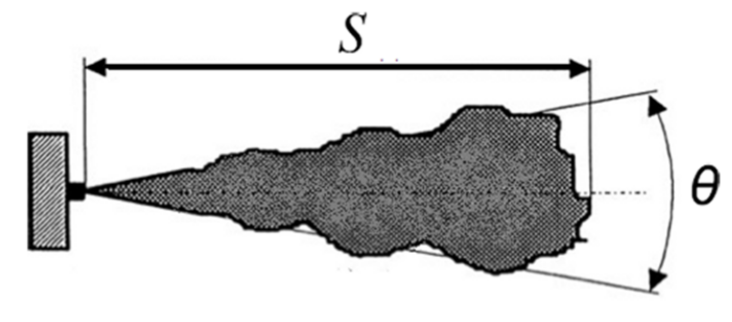
The injection system aims at delivering fuel with the proper timing and quantity required by the combustion process and represents a fundamental element of the engine in contributing to emissions and performances [1]. Therefore, particular care must be taken with the injection process, mainly for compression ignition engines, whose essence lies in the introduction of finely atomized fuel into the compressed air inside the cylinder. For diesel engines, indeed, fuel spray plays a major role since its characteristics are strictly related to the combustion process [2]. Sprays can be characterized in terms of microscopic parameters, such as droplets size and velocity, or from a macroscopic perspective. In this latter case, the geometrical description of the overall jet is provided, namely, in terms of tip penetration length (S) and cone angle () as sketched in Figure 1.
While penetration is univocally defined and easily measured as the travelled distance by the tip of the spray into still air [3], the measurement of the cone angle is quite challenging and, among the scientific community, there is no agreement in defining such quantity. It can be measured as the angle formed by two straight lines emerging from the discharge hole and tangent to the spray contour, as a function of the penetration, or as a function of the nozzle diameter. Alternatively, it can be measured by fitting two straight lines to the spray contour or even as the apex angle of an isosceles triangle having the corresponding spray area at a given percentage of the penetration length. A comprehensive description and comparison of different spray angle definitions can be found in [4] where a variation up to 95% has been observed in the cone angle evaluated by different methods. This disagreement arises from the fact that the spray cone features irregular and faded boundaries, thus making it intrinsically difficult to discern what is to be considered as spray from the surrounding.
Among different experimental approaches ranging from mechanical to electrical solutions [3], macroscopic spray characterization is mainly performed by means of optical techniques [5], being these methods non-intrusive and hence allowing for the study of the jet without affecting its own evolution. Amongst the optical approaches, direct visualization technique, such as high-speed photography, is widely used. The output of such technique is a time series of digital images, commonly in grey tones, of the evolving spray, which must be post-processed to extract the spray characteristic. The first step into the analysis is to isolate the spray from the background.
The operation of separating a subject from the surrounding image is referred to as segmentation and represents one of the most challenging tasks in image processing [6]. Two main approaches can be followed in pursuing image segmentation: subdivide the image in regions according to a sudden change in the intensity of pixels (e.g., looking for edges); categorize the pixels showing similar properties into classes [6]. Thresholding belongs to the second group and plays a central role in image segmentation. In the image thresholding, every pixel is assigned either to the subject or to the background, by comparing its intensity to a given threshold T. The resulting output is a binary image in which every pixel shows a 0 or 1 value depending on the assigned ensemble. Over the decades, a lot of solutions have been proposed to select the proper threshold and some of them have been applied to diesel spray images.
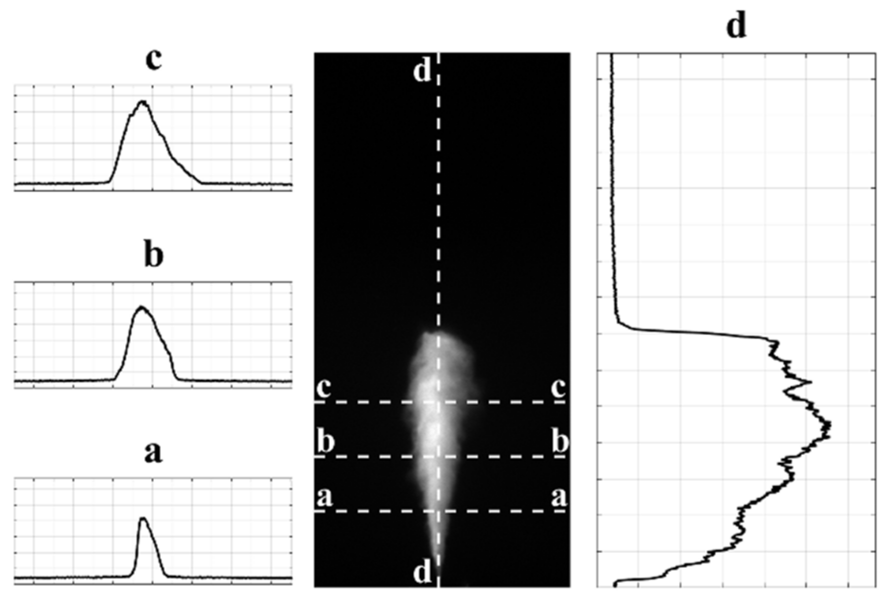
The threshold is manually selected as a constant value for all of the image set on the basis of the visual quality of the result in [7,8,9]. This solution cannot be considered as a good choice as the illumination and, therefore, the pixel intensity varies between different images. In addition, results are sensitive to the experimenter interaction. To overcome such limitation, some authors implement more refined algorithms for automatic threshold selection, relying either on the shape of the image histogram [10] or on statistical approaches as the Likelihood Ratio Test [11,12,13], the Maximum Entropy Method [14,15] or the Otsu’s Method [16]. These methods, which arise for general segmentation purposes, show good performances also in segmenting spray images. However, different algorithm results in a different threshold level, which in turn leads to different macroscopic spray parameters, mainly affecting the cone angle [4,17]. A better understanding can be achieved considering a typical spray image and the corresponding pixel intensity over three transverse profiles (Figure 2a–c) and along the longitudinal direction (Figure 2d). Considering the longitudinal profile, it is evident that the spray leading edge is characterized by a steep slope whereas in the transverse direction, the image intensity shows a smooth transition. Therefore, a slight change in the threshold slightly influences the position of the pixels in the spray tip, while it greatly affects the side contour and consequently the cone angle. A variation of up to 24% can be observed when the same cone angle definition is considered as two different segmentation techniques are adopted [17].
The abovementioned considerations led to the development of the present work. The goal is to develop a method for the spray characterization that does not require the evaluation of the spray contour and does not rely over thresholding.
In the present paper, an algorithm based on a shape similarity analysis between the real spray images and known artificial images is proposed. Images coming from two different experiments have been analyzed and the obtained penetration and cone angle are compared with results obtained by implementing the Otsu’s thresholding technique and four definitions for the cone angle.
2. Algorithm
Regardless of the considered segmentation technique, the desired output is not the description of the actual spray boundary but rather an overall description of the spray shape, given by penetration and cone angle. The latter can be outlined as a conical region, surmounted by a semi-elliptical or by a circular head [18,19]. Therefore, the goal of the macroscopic spray characterization is to obtain such simplified description. The technique proposed in the present paper aims at obtaining the abovementioned shape.
A similar approach is followed in [9,20] where the cone angle definition is associated to those of a symmetrical triangular shape, whose area is proportional to the binarized spray image one. Therefore, this method does not imply that the shape of the resulting model is close to the actual one or that the obtained value is independent on the used segmentation algorithm.
The proposed method is rooted on the technique described in [21] where a basic face recognition algorithm is used to select the threshold level T in order to perform image segmentation and obtain the spray boundary. In this method, a database of binary images is created case by case, by thresholding the original image with different intensity levels. The images are hence represented as vectors, and then, the closest match between the original image and the best black and white version is obtained. The macroscopic spray parameters are than evaluated by processing the resulting boundary in accordance to one of the possible definitions of such parameters.
In the present paper, the database is no longer created image by image but is made up of artificial binary spray images just once. The method looks for the closest match between the original image and its simplified binary version and, given that the parameters of such images are a priory known, no further analysis is required to evaluate the spray parameters.
The database must be representative of all of the possible spray shapes. Considering the whole injection event, it is clear that a database containing all of the significant angles, penetrations and shapes of the leading edge becomes so wide to be unmanageable. In order to reduce the database dimensions, while maintaining its representativeness, the penetration length of the artificial sprays can vary within a range centered around half of the image height. Then, a scaling step of the original spray is introduced in order to make the real image and the artificial ones comparable.
The goal is to characterize the volume of the spray through one of its projections (e.g., an image). Therefore, only symmetrical spray shapes have been considered. The asymmetries encountered in a single image, which are often due to the illumination pattern rather than to the spray itself, cannot be extended to the entire spray. Figure 3 shows a sketch of the artificial images, which constitute the database. Sprays are obtained by varying the penetration S, the angle θ and the ellipse semi-axes ξ.
It is worth mentioning that the size of the artificial images must be the same as that of the real spray images. This is not a limiting factor: The tested image is simply to be resized to be compared to an existing database afore starting the processing. Still, images must have the same aspect ratio (e.g., the same ratio between pixel height h and width w).
An image of size can be represented as a column vector of dimensions . By following this representation, any image can be considered as a point in the N-dimensional images space. This high dimensionality space is representative of images depicting whatever subject. Images showing similar features, like sprays, are located into a sub-space, i.e., into a smaller region of this space. The idea behind the method is to compute the coordinate system that efficiently describes such cluster. This operation is referred to as Principal Component Analysis, and is commonly used for image compression. It also turns out to be successfully used for recognition purposes [22].
Let us consider a database made up of n binary images whose images are represented as vectors of size . The mean database image is:
The deviation matrix D of the database can be evaluated as:
where the columns are the deviation vectors of each database image with respect to the mean image. The following formula is used for the computation:
The covariance matrix C can be obtained by matrix D:
The principal components of the database are the eigenvectors , also referred to as eigenimages, of the covariance matrix. As stated before, the principal components represent a coordinate system that easily allows for the representation of the data (database image). The computation of the eigenvalues is extremely time-consuming, as it requires the solution of a polynomial equation of order being N representative of the image size (commonly 1024 × 768 or larger). As reported in [22], given that the covariance matrix is obtained from a database of only n images, instead of the covariance matrix C, the reduced matrix B can be used:
Given that , the benefit derived from considering B instead of C is evident.
Each image of the database can be optimally approximated in terms of a linear combination of the M eigenvectors:
The original spray image, , is similar to the images of the database. Therefore, one could think to also provide a description of by using the computed coordinate system:
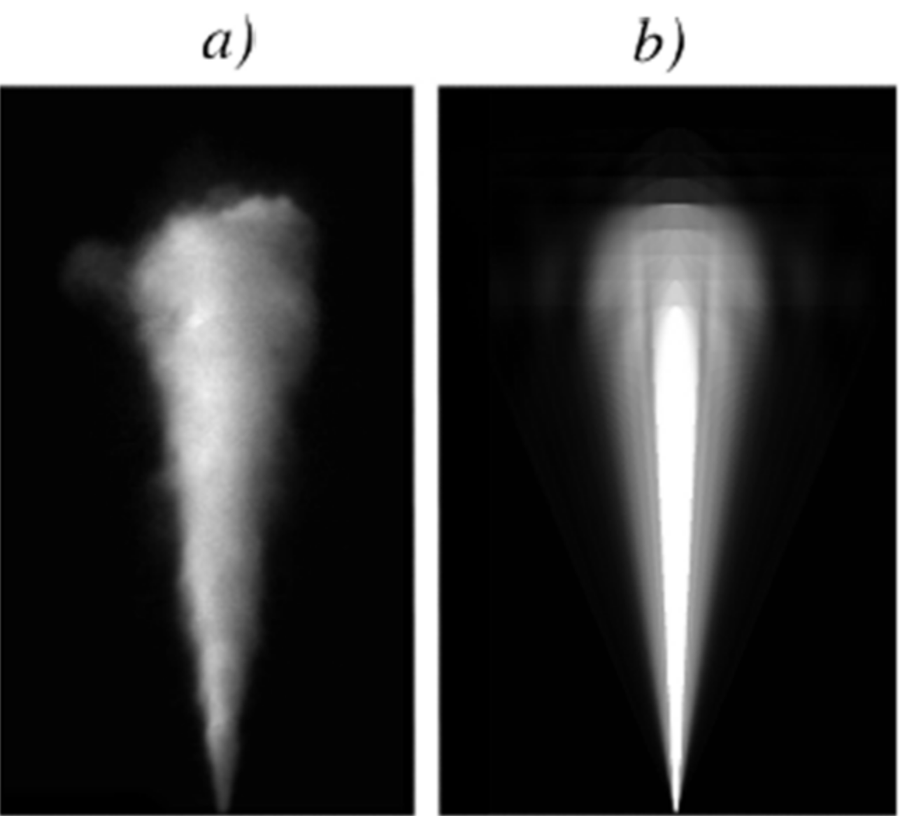
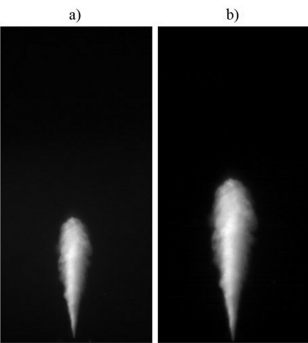
Figure 4 shows a spray image (a) and its approximation (b) obtained using Equation (7).
This reconstruction procedure can be seen as a projection of image or over the computed image space. By means of this operation, images become comparable, and the best match can be found by evaluating the minimum Euclidean distance between the spray image projection and every database reconstructed image :
where and are the projection weights to scale each eigenvector. The latter are computed as:
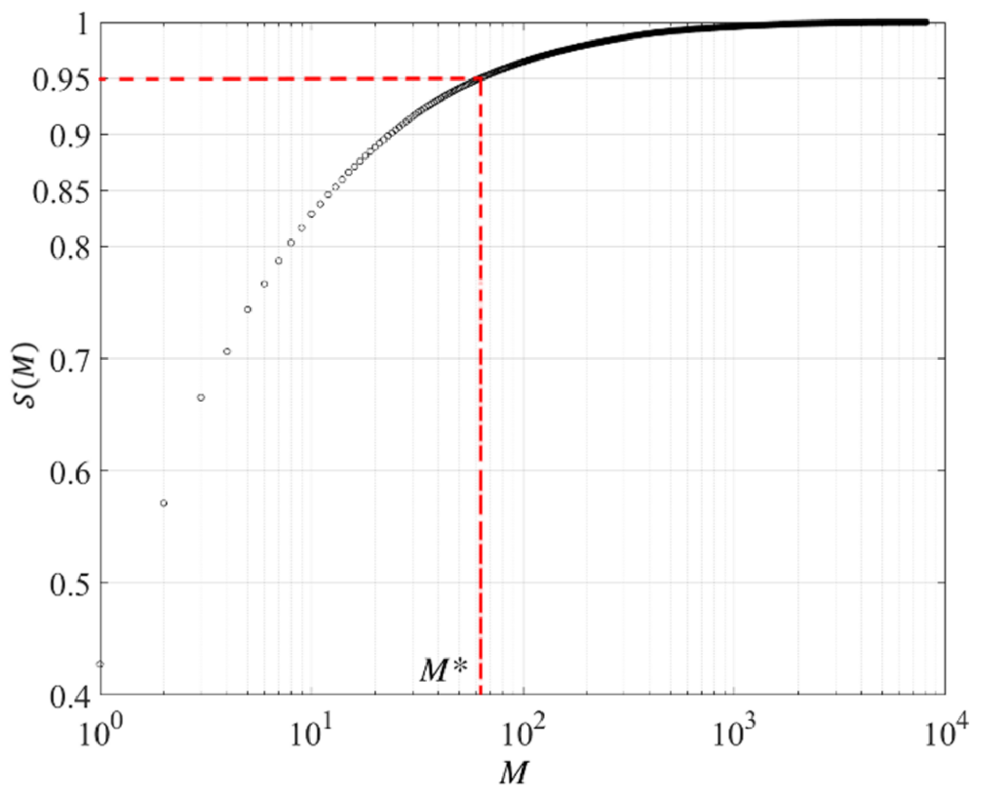
Each eigenvalue of the reduced covariance matrix B describes a certain percentage, proportional to its magnitude, of the variation of the data in the direction given by the corresponding eigenvector. Therefore, to properly compare two vectors, it is unnecessary to consider all of the M eigenvectors. A smaller set M* associated to the most significant eigenvalues is sufficient. Therefore, M* is selected as the lowest number for which the sum of the first M eigenvalues, divided by the sum of all the eigenvalues, is larger than a value k (e.g., 95%).
Figure 5 shows the cumulative sum of the eigenvalues computed for a database made up of 8000 artificial images. Considering a percentage k = 95%, a number M* = 63 of eigenvalues can be considered.
The database construction, the eigenvalues-eigenvectors computation and the projection over the image space (e.g., the evaluation of the coefficients) has to be performed only once. For subsequent analyses, it is enough to store the M* eigenimages, the weights as well as the mean image . A spray image analysis consists only in computing from Equation (8) and hence finding out the minimum distance using Equation (9). Since the artificial image is geometrically known in advance no further analysis is required.
3. Spray Image Processing
3.1. Required Preliminary Data
Before processing the image, some parameters are required, namely, its spatial resolution (pixels/mm) and the coordinates of the nozzle hole. The size of the image is than matched to the size of the database images, if required.
3.2. Image Pre-Processing
3.2.1. Background Correction
In order to correct the effect of uneven illumination and to eliminate unwanted reflections, background has to be corrected. Different approaches can be followed for this purpose. A common solution is to subtract a mean background image, from the image under processing. In our test the background is estimated image by image, by bilinear interpolation of the mean value of the 5 pixels columns on both side of the image (Figure 6a,b) shows the estimated background.
3.2.2. Spray Scaling
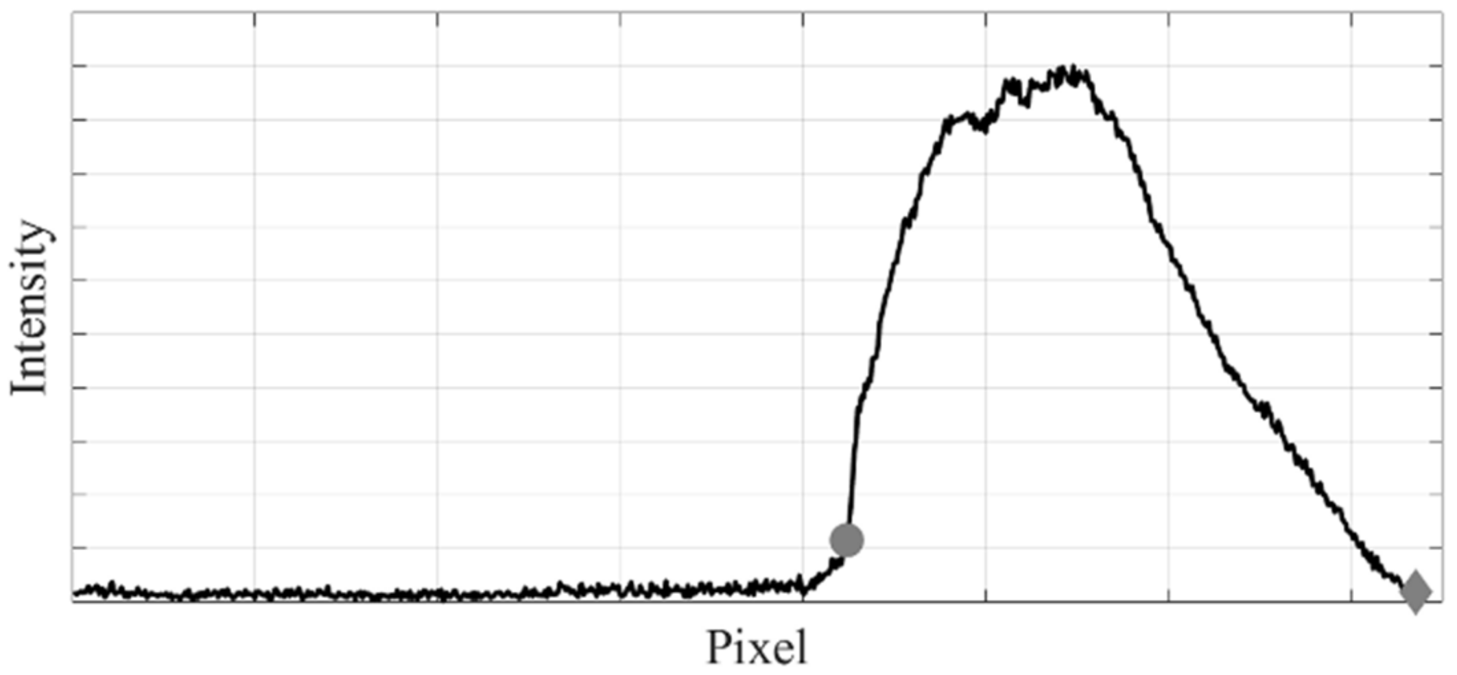
As mentioned in Section 2, in order to make the real image and the artificial ones comparable, the spray must be scaled in order to occupy almost half of the image’s pixels height. Therefore, the scaling factor is obtained by roughly estimating the penetration length from the intensity profile along the axial direction (distance between the circle and the diamond in Figure 7). This first estimation has not to be extremely accurate being the actual penetration evaluated by the algorithm, which takes into account the variation of such parameter.
3.3. Macroscopic Spray Parameters Estimation
As final step, the scaled image is processed using the proposed algorithm and the projection weights (Equation (9)) are computed. The corresponding artificial image (simplified contour) is hence determined (Equation (8)).
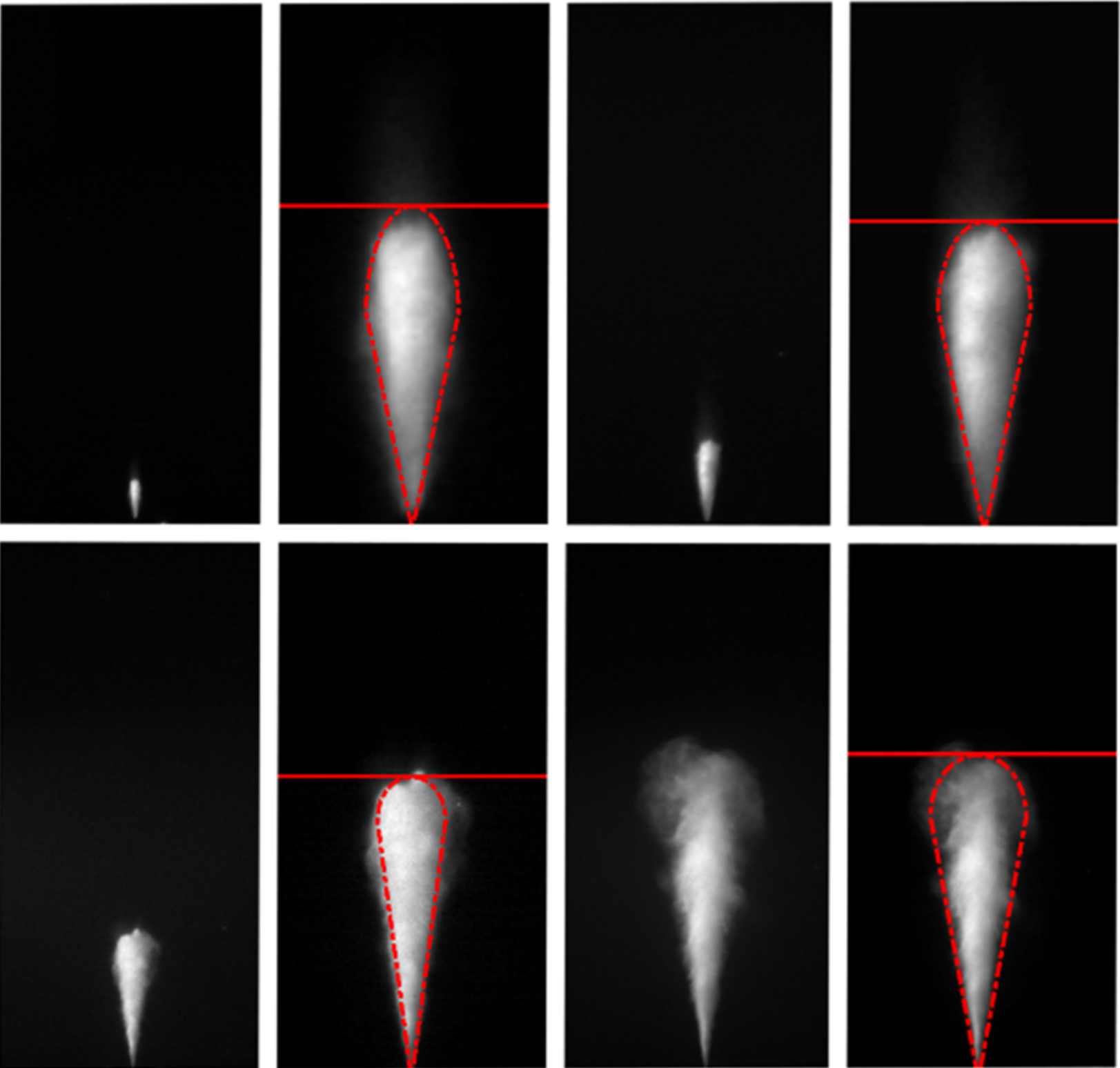
Figure 9 shows some results obtained with the proposed algorithm. The obtained contour and a line representative of the penetration length are superimposed to the scaled image. The actual penetration value must be rescaled by means of the scaling factor used for the transformation (Section 3.2.2). As it is worth observing from these images, thanks to the scaling step, the proposed method is able to properly work in the whole range.
4. Experimental Setup
4.1. Imaging System
Image acquisition is performed by a PCO-SensiCam Double Shutter digital camera. The camera has a monochromatic 12-bit CCD sensor with adjustable resolution up to 1280 × 1024 pixels. The physical pixel size is 6.7 µm × 6.7 µm. The yielding image spatial resolution is 11 px/mm. The camera dynamic range has been kept constant over the entire measurement campaign. A single image has been acquired for every injection event and the whole spray evolution has been acquired by synchronizing the light source and the camera at different times from the start of the injection. At least 20 images were acquired for each time step. Illumination is achieved by a high intensity Xenon lamp with a duration of about 2 µs.
4.2. Spray Test Rig
The injector is mounted in a constant volume chamber designed for pressures up to 6 MPa. A spherical joint allows the alignment of the spray plume under investigation with the vertical axis of the chamber. Three optical access made of BK7 allow lighting and imaging. Figure 10 shows the layout of the injection chamber.
Illumination is provided by side, and the digital camera collects the scattered light from the frontal window. On the opposite side of the lamp, a mirror reflects the incident light providing a symmetrical illumination.
The nozzle has 5 cylindrical holes of diameter D = 133 µm. A nozzle cap is used to isolate a single plume. This is necessary because the lateral lighting will project over the spray under investigation shadows of the other plumes.
The vessel is filled with nitrogen kept at a temperature of 18 ± 1 °C and at a pressure of 3 ± 0.5% MPa resulting in an ambient density of 34.7 ± 0.2 kg/m3.
4.3. Test Points
Two experimental conditions were considered. Rail pressure and injector energizing time are reported in Table 1.
4.4. Image Database
In order to check any database dependence, analyses have been performed considering two different databases whose parameters are reported in Table 2:
For both databases, the semi axes ξ of the front edge ellipse varies from 0 to 1/3 of the penetration length in 8 steps. Furthermore, penetration shows a variation of about ±8% around its mean value (half of the image height) discretized in 8 steps.
4.5. Cone Angle and Penetration Definition
The proposed method has been compared with the Otsu’s thresholding. Table 3 sums up the four adopted cone angle definitions.
Penetration S is evaluated from the binarized images, as the distance from the hole of a line orthogonal to the spray axis that individuates a region including the 99% of white pixels (the spray). Cone angle definitions (b) and (d) are based on such definition.
5. Results
5.1. Database Effect
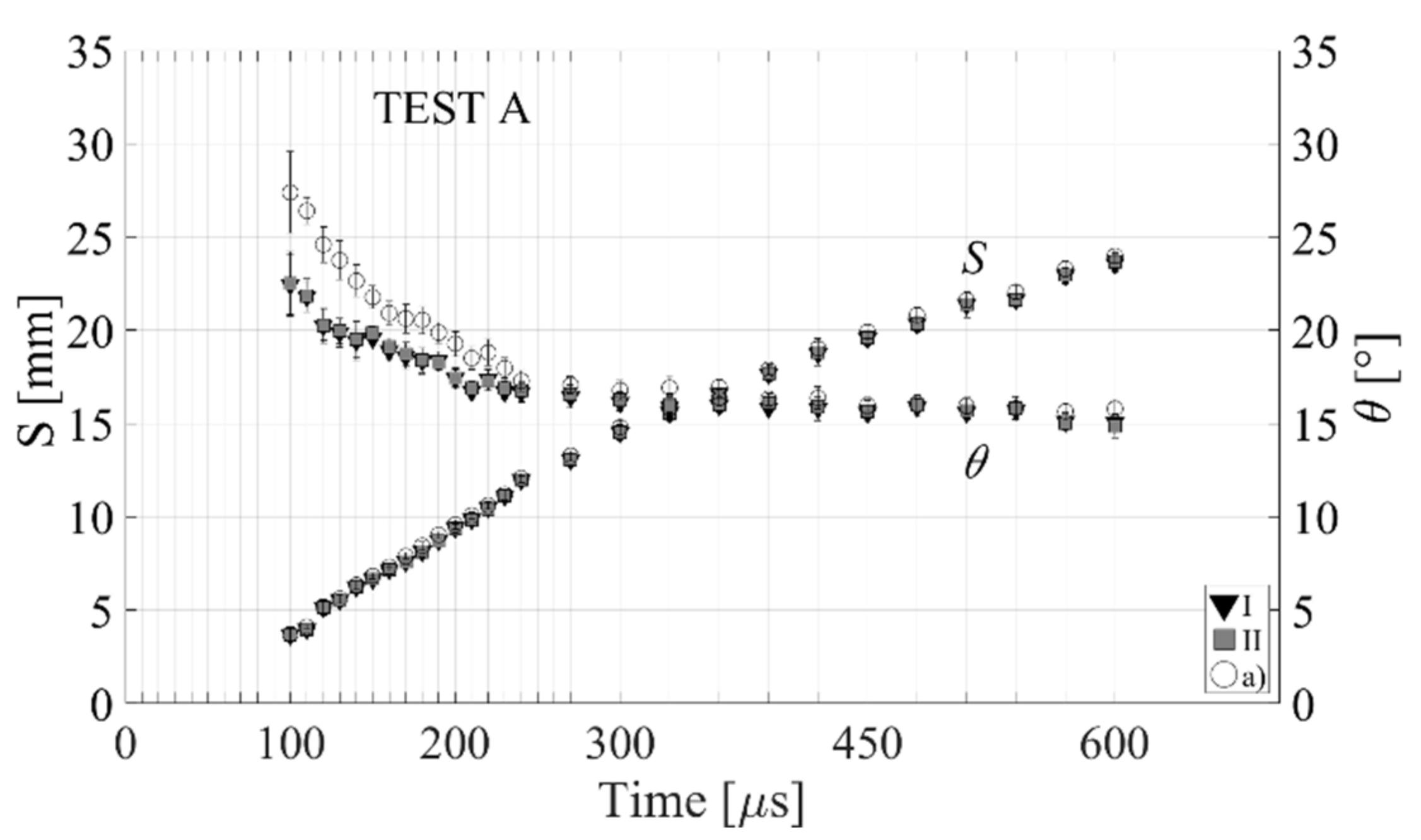
Figure 11 and Figure 12 show the temporal evolution of the penetration S and of the cone angle for test points in Table 1 Markers represent the mean value of 20 observations, whose standard deviation is represented by the vertical bars. Results obtained by using databases I and II (filled markers) are compared to those obtained by implementing the Otsu’s threshold and definition (a) of the cone angle (empty circles).
These figures show that penetration and cone angle obtained by using the two databases are overlapped. This evidence proves that the proposed method does not depend on the database construction, which, on the other hand, should obviously cover the whole expected cone angle range.
The penetration trends obtained by the synthetic database method are the same obtained by implementing the Otsu thresholding and the definition of penetration given in Section 4.5.
5.2. Image Intensity Effect
As stated in the introduction, methods based on thresholding are influenced by the selected threshold level, which is obtained, by following different possible approaches, from the image histogram (the pixel intensity distribution). In order to check the level of dependence of the proposed algorithm from the histogram, image intensity has been scaled by a factor ranging from 1 to 0.1. This operation modifies the pixel intensity distribution that condensates towards zero with a loss of information. As an example, Figure 13 shows the obtained cone angle value as a function of the intensity scaling factor for the proposed method and the Otsu’s thresholding combined with the angle definitions in Table 3. For intensity multiplier value equal to 0.1, the resulting cone angle is out of scale. As it is clear, the proposed method (triangular markers) is minimally influenced by the histogram modification while the Otsu’s thresholding is greatly affected by the operation.
5.3. Methods Comparison
Figure 14 and Figure 15 compare the cone angle trends obtained using database I to those obtained by adopting the Otsu’s thresholding and the four definitions of the cone angle.
As it stems from the charts, all methods show similar trends, except for method (c). The cone angle definition (c) is associated to a fixed distance multiple of the hole’s diameter. Therefore, no data are available for spray having a penetration lower than this value. The proposed method shows a steady state value comparable to those of all the other method. The same variability in the mean value can be registered among different technique. Therefore, it can be attributed mainly to the shot-to-shot variation.
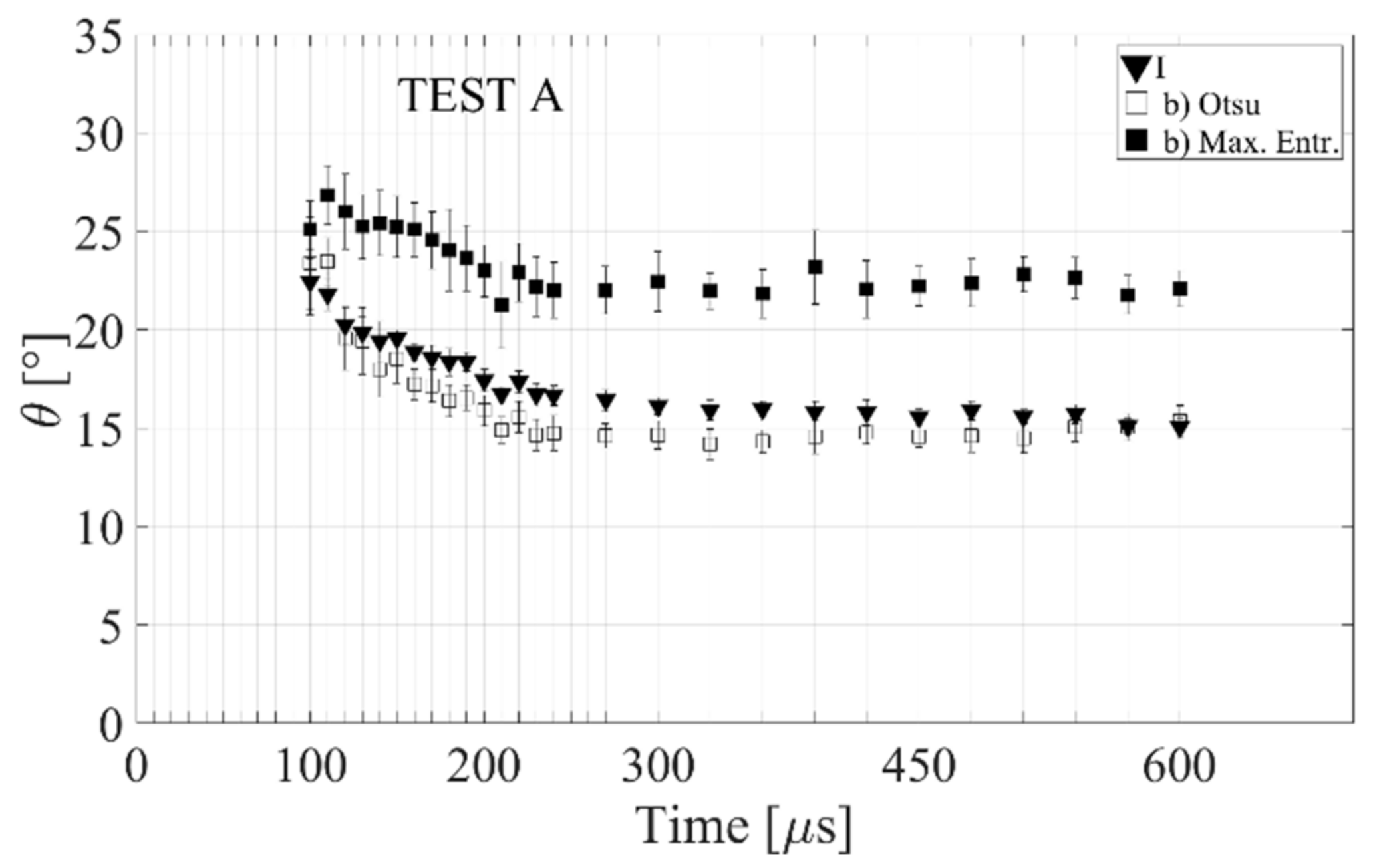
It can be noticed that the database method trends are closer to those obtained with the angle definition (b). This consideration should not be generalized; in fact, it must be stressed out that trends (a) to (d) are strictly dependent on the method used to obtain the spray contour, which in this case is the Otsu’s thresholding. As an example in Figure 16 the same cone angle definition (b) is applied when the spray contours have been evaluated by the Otsu’s method and the Maximum Entropy Thresholding. The differences in the final estimation of the cone angle are evident.
6. Conclusions
A method for diesel spray macroscopic parameter estimation from digital images has been developed. It relies over principal component analysis which is an extensively used tool in digital image processing framework. The method looks for the best match between the original spray image and an artificial one within a known shape database. Once the simplified spray shape is obtained, it being known in advance, cone angle and penetration are directly evaluated.
The proposed method evaluates the macroscopic spray parameters without segmenting the image and has an intrinsic cone angle definition based on a symmetric spray shape.
The method requires real spray images to have the same size of those of the database. This requirement is not a real limitation. It can be easily solved by scaling the size of original images to match those of the database prior to starting the image processing. However, original and database images must have the same aspect ratio. It has been shown that the database size does not affect the macroscopic parameters’ estimation.
The proposed method has been compared with the uttermost popular Otsu’s thresholding procedure and four definitions of the cone angle. The obtained results show that the proposed method is equivalent to traditional thresholding-based techniques, and it shows a negligible dependence on the image histogram manipulation.
Author Contributions
Conceptualization, writing—original draft preparation, writing—review and editing, A.B. and C.D.
Funding
This research received no external funding.
Acknowledgments
The authors would like to thank Daniela Anna Misul for revising the manuscript.
Conflicts of Interest
The authors declare no conflict of interest.
References
- Pierpont, D.A.; Reitz, R.D. Effects of Injection Pressure and Nozzle Geometry on D.I. Diesel Emissions and Performance. SAE Trans. 1995, 104, 1041–1050. [Google Scholar]
- Heywood, J.B. Internal Combustion Engine Fundamentals; McGraw-Hill: New York, NY, USA, 1988; ISBN 007028637X. [Google Scholar]
- Lefebvre, A.; Mcdonell, V. Atomization and Sprays, 2nd ed.; CRC Press: Boca Raton, FL, USA, 2017; p. 300. [Google Scholar]
- Ruiz-Rodriguez, I.; Pos, R.; Megaritis, T.; Ganippa, L.C. Investigation of Spray Angle Measurement Techniques. IEEE Access 2019, 7, 22276–22289. [Google Scholar] [CrossRef]
- Soid, S.N.; Zainal, Z.A. Spray and combustion characterization for internal combustion engines using optical measuring techniques—A review. Energy 2011, 36, 724–741. [Google Scholar] [CrossRef]
- Gonzalez, R.C.; Woods, R.E. Digital Image Processing, 3rd ed.; Pearson Prentice Hall: Upper Saddle River, NJ, USA, 2008; ISBN 978-0131687288. [Google Scholar]
- Shao, J.; Yan, Y.; Greeves, G.; Smith, S. Quantitative characterization of diesel sprays using digital imaging techniques. Meas. Sci. Technol. 2003, 14, 1110–1116. [Google Scholar] [CrossRef]
- Morgan, R.; Wray, J.; Kennaird, D.A.; Crua, C.; Heikal, M.R. The Influence of Injector Parameters on the Formation and Break-Up of a Diesel Spray. SAE Trans. 2001, 110, 389–399. [Google Scholar]
- Naber, J.; Siebers, D.L. Effects of Gas Density and Vaporization on Penetration and Dispersion of Diesel Sprays; SAE Technical Paper Series; SAE International: Troy, MI, USA, 1996; Volume 1. [Google Scholar]
- Cronhjort, A.; Wåhlin, F. Segmentation algorithm for diesel spray image analysis. Appl. Opt. 2004, 43, 5971. [Google Scholar] [CrossRef]
- Payri, F.; Pastor, J.V.; Palomares, A.; Juliá, J.E. Optimal feature extraction for segmentation of Diesel spray images. Appl. Opt. 2004, 43, 2102. [Google Scholar] [CrossRef] [PubMed]
- Pastor, J.V.; Arrègle, J.; Palomares, A. Diesel spray image segmentation with a likelihood ratio test. Appl. Opt. 2001, 40, 2876. [Google Scholar] [CrossRef] [PubMed]
- Pastor, J.V.; Arrègle, J.; García, J.M.; Zapata, L.D. Segmentation of diesel spray images with log-likelihood ratio test algorithm for non-Gaussian distributions. Appl. Opt. 2007, 46, 888. [Google Scholar] [CrossRef] [PubMed]
- Seneschal, J.; Maurin, B.; Champoussin, J.C.; Ducottet, C. A Fully Automatic System for the Morphology Characterization of High Pressure Diesel Sprays; SAE Technical Paper Series; SAE International: Troy, MI, USA, 2004; Volume 1. [Google Scholar]
- Kapur, J.N.; Sahoo, P.K.; Wong, A.K.C. A new method for gray-level picture thresholding using the entropy of the histogram. Comput. Vis. Graph. Image Process. 1985, 29, 273–285. [Google Scholar] [CrossRef]
- Otsu, N. A Threshold Selection Method from Gray-Level Histograms. IEEE Trans. Syst. Man. Cybern. 1979, 9, 62–66. [Google Scholar] [CrossRef]
- Macian, V.; Payri, R.; Garcia, A.; Bardi, M. Experimental Evaluation of the Best Approach for Diesel Spray Images Segmentation. Exp. Tech. 2012, 36, 26–34. [Google Scholar] [CrossRef]
- Rubio-Gómez, G.; Martínez-Martínez, S.; Rua-Mojica, L.F.; Gómez-Gordo, P.; de la Garza, O.A. Automatic macroscopic characterization of diesel sprays by means of a new image processing algorithm. Meas. Sci. Technol. 2018, 29. [Google Scholar] [CrossRef]
- Delacourt, E.; Desmet, B.; Besson, B. Characterisation of very high pressure diesel sprays using digital imaging techniques. Fuel 2005, 84, 859–867. [Google Scholar] [CrossRef]
- Araneo, L.; Coghe, A.; Brunello, G.; Cossali, G.E. Experimental Investigation of Gas Density Effects on Diesel Spray Penetration and Entrainment. SAE Trans. 1999, 108, 679–693. [Google Scholar]
- Dongiovanni, C.; Negri, C.; Pisoni, D. Macroscopic Spray Parameters in Automotive Diesel Injector Nozzles With Different Hole Shape. In Proceedings of the ASME 2003 Internal Combustion Engine Division Spring Technical Conference, Salzburg, Austria, 11–14 May 2003; American Society of Mechanical Engineers: New York, NY, USA, 2003; pp. 77–85. [Google Scholar]
- Turk, M.; Pentland, A. Eigenfaces for Recognition. J. Cogn. Neurosci. 1991, 3, 71–86. [Google Scholar] [CrossRef] [PubMed]
Figure 1.
Generic definition of macroscopic spray parameters.

Figure 2.
Transverse (a–c) and longitudinal (d) intensity profile of a typical diesel spray image.

Figure 3.
Artificial spray parametrization.

Figure 4.
(a) Original Image. (b) Reconstructed version using database.

Figure 5.
Cumulative normalized sum of the eigenvalues.

Figure 6.
(a) Original image. In red pixels columns for background estimation. (b) Estimated background (intensity adjusted for visualization purposes).
Figure 6.
(a) Original image. In red pixels columns for background estimation. (b) Estimated background (intensity adjusted for visualization purposes).

Figure 7.
Penetration estimation for scaling.

Figure 8.
(a) Original image. (b) Scaled Image.

Figure 9.
Spay contour evaluated by using the proposed method at different time step.

Figure 10.
Experimental layout.

Figure 11.
Test A: Penetration and cone angle temporal evolution.

Figure 12.
Test B: Penetration and cone angle temporal evolution.

Figure 13.
Intensity level effect.

Figure 14.
Test A: Comparison of the cone angle trends for the different methods.

Figure 15.
Test B: Comparison of the cone angle trends for the different methods.

Figure 16.
Test A: Effect of the thresholding algorithm.


Table 1.
Test points.
| Test | ||
|---|---|---|
| A | 60 | 380 |
| B | 135 | 600 |
Table 2.
Database Parameter.
| Database | |||
|---|---|---|---|
| I | 1 | 35 | 0.2 |
| II | 5 | 45 | 0.4 |
Table 3.
Adopted cone angle definition.
| Method | Description | Ref. |
|---|---|---|
| (a) | Angle between two lines excluding 2.5% of white pixels on each side of the binary image | [21] |
| (b) | Line fitting the spray boundaries at 0.6 S | [4,17] |
| (c) | Line fitting the spray boundaries at 60 D (no data available for S < 60 D) | [3,4] |
| (d) | Apex-angle of a triangle having height equal to 0.5 S and corresponding equivalent area | [4,9,20] |
© 2019 by the authors. Licensee MDPI, Basel, Switzerland. This article is an open access article distributed under the terms and conditions of the Creative Commons Attribution (CC BY) license (http://creativecommons.org/licenses/by/4.0/).
Share and Cite
MDPI and ACS Style
Bottega, A.; Dongiovanni, C. Diesel Spray Macroscopic Parameter Estimation Using a Synthetic Shapes Database. Appl. Sci. 2019, 9, 5248. https://0-doi-org.brum.beds.ac.uk/10.3390/app9235248
AMA Style
Bottega A, Dongiovanni C. Diesel Spray Macroscopic Parameter Estimation Using a Synthetic Shapes Database. Applied Sciences. 2019; 9(23):5248. https://0-doi-org.brum.beds.ac.uk/10.3390/app9235248
Chicago/Turabian StyleBottega, Andrea, and Claudio Dongiovanni. 2019. "Diesel Spray Macroscopic Parameter Estimation Using a Synthetic Shapes Database" Applied Sciences 9, no. 23: 5248. https://0-doi-org.brum.beds.ac.uk/10.3390/app9235248
Note that from the first issue of 2016, this journal uses article numbers instead of page numbers. See further details here.