A Novel Design of Fractional PI/PID Controllers for Two-Input-Two-Output Processes

Abstract

In this paper, a new formulation of fractional order proportional integral (PI)/ proportional integral derivative (PID) controller is proposed. The proposed controller will be justified for some well-known two-input-two-output (TITO) processes. In order to deal with interactions between process variables in a multivariable system, as well as multiple delay times in process transfer functions, the simplified decoupling Smith predictor (SDSP) structure is also used. The issue of decoupling realizability is solved by the PSO algorithm and fractional order processes are also suggested for model reduction. The tuning rules of the controller are derived in analytical terms based on the internal model control (IMC) structure. The effectiveness and robust stability of the proposed approach are illustrated by comparing it with other methods. To have a fair comparison, the robustness criterion using the M-Δ structure with μ-synthesis is adopted and the μ value of the proposed method is always kept smaller than the value of the others.

1. Introduction

In recent years, the fractional-order proportional-integral-derivative (FOPID) controller, which is first proposed by Podlubny [1], has attracted more attention of many researchers in the field of control systems. The FOPID has five tuning parameters including proportional, integral, derivative gain and fractional orders of the integral and derivative terms. In the special case, when the fractional orders are equal to unity, the controller becomes a conventional proportional-integral-derivative (PID). Therefore, it is considered as a generalization of the PID controller to non-integer orders, and it provides more flexibility in controller design as well as better dynamic performances and robustness compared with the conventional one [1,2,3,4]. Due to more tuning parameters, it is harder to derive analytical tuning rules for the controller. Different tuning methods have been suggested to solve this kind of problem [5,6,7,8,9,10,11,12,13,14]. However, most of them are used to deal with single-input single-output (SISO) systems. In this paper, a novel structure of FOPID is proposed to apply for two-input two-output (TITO) processes.

In this work, the simplified decoupling Smith predictor structure (SDSP) for multivariable processes proposed by Chuong et al. [15] is adopted to deal with interactions between process variables as well as multiple time delays of the processes. The realizability problem plays a crucial role in implementing a decoupler because of the requirements of being stable and proper of all its internal transfer functions. To overcome this issue, therefore, many researchers proposed the approximation approaches such as prediction error method (PEM), linear least square in frequency domain [16], and coefficient matching (CM) [17,18]. However, these mentioned methods are only suitable for reducing to integer-order transfer functions. In this paper, to enhance dynamic behaviors of decoupled systems, fractional order processes are addressed to be the equivalent transfer functions of the decoupled elements. Therefore, the whole controller structure used in this work is called fractional simplified decoupling Smith predictor (F-SDSP). The particle swarm optimization (PSO) algorithm for approximation procedure proposed in [15] is employed to find out the parameters of approximated fractional functions. Bouyedda et al. [14] performed a similar work by using the Genetic Algorithm (GA) to reduce a high integer-order transfer function of a SISO system to a lower fractional-order one. Besides, to improve the performances of a system, a generalized PI/PID controller, known as fractional-order PI/PID (FOPI/FOPID) controller, is suggested for decoupled systems.

In the last two decades, various methods for FOPI/FOPID design were proposed in the field of process control. Among those, there are two prominent approaches: The internal model control (IMC)-based procedure and the gain and phase margin-based frequency domain design. The first one uses IMC scheme to reduce the number of tuning parameters; and normally, there is only one parameter left needs to be tuned based on some criteria of robust performances such as maximum peak (M_p) or maximum sensitivity (M_s) [11,12,13,14]. The second one uses constraints on phase margin, gain crossover frequency and the flat phase around the gain crossover frequency to ensure robustness performance [5,6,7,8,9,10]. The most disadvantage of the latter is that those constraints are only enough to solve three tuning parameters which means merely to be appropriate to a FOPI controller (a FOPID has five tuning parameters). Furthermore, most of the previous works only deal with SISO processes. Therefore, expanding some existing design methods to multivariable processes is necessary and deserves to attract more attention from researchers.

In this paper, the IMC-based FOPI/FOPID design is adopted to find out analytical tuning rules of both FOPI and FOPID controllers for TITO processes. Moreover, as mentioned in the previous work [15], one of the advantages of the proposed structure (SDSP) is to remove dead time out of the diagonal elements of the decoupled transfer function matrix. Therefore, only the delay-free parts of it are addressed to design the controllers. Note that, in this work, the fractional order transfer function (FOTF) is used instead of the integer order one. In addition, to evaluate the robustness stability of the proposed method, the M-Δ structure normally used for integer order systems [15,16,17,18,19,20,21,22] is also applied for fractional order ones. Then, the μ-synthesis, known as structured singular value (SSV), is employed to measure the robustness of the fractional controllers for multivariable processes with multiplicative output uncertainty.

This paper is organized as follows. Section 2 is briefly introduced fractional order calculus with the Oustaloup recursive algorithm to approximate the fractional operator. Furthermore, the general structure of the controller is presented with reduced models based fractional order. A new fractional order PID controller is also proposed and then analytical tuning rules are derived based on the internal model control structure. Some criteria to evaluate the system performances are mentioned in Section 2 as well. Section 3 presents the simulations of some well-known TITO processes to justify the effectiveness and robustness of the proposed method. Finally, conclusions are given in Section 4.

2. Materials and Methods

2.1. Fractional Order Calculus

Fractional calculus is a generalization of ordinary calculus by extending the integration and differentiation order to the non-integer order. It has been developed for a long time as a field of mathematics and only applied for control engineering in the last two decades. It presented a fractional operator ${}_a^{}{D}_t^v$ where a and t are the limits and $v$ is the fractional order ($v\in R$). There are several definitions for fractional operator but the most commonly used one was proposed by Riemann and Liouville [3]. It is defined as follow:

$${}_a^{}{D}_t^{v}f(t)=\frac{1}{\mathsf{\Gamma }(n-v)}\frac{d}{d{t}^n}{\displaystyle \underset{a}{\overset{t}{\int }}\frac{f(\mathsf{\tau })}{{(t-\mathsf{\tau })}^{v-n+1}}dt, n-1<v<n}$$

(1)

where $\mathsf{\Gamma }(•)$ represents the Euler’s gamma function; with a positive $v$, the fractional operator denotes fractional derivative, and a negative $v$ represents fractional integral.

The Laplace transformation is used for Equation (1) under the assumption that all initial conditions are zero. Its result has the form given in (2):

$$L\left\{{}_a^{}{D}_t^{v}f(t)\right\}=s^{v}F(s)$$

(2)

Consider a SISO, linear time invariant fractional order system described by a typical fractional order differential equation (FODE) as follow:

$${\displaystyle \sum _{i=0}^n{a}_i{D}_0^{v_i}y(t)=}{\displaystyle \sum _{i=0}^m{b}_i{D}_0^{{\lambda }_i}u(t)}$$

(3)

where y(t) and u(t) are the output and input respectively; a_i, b_i are constant coefficients of the system; $v_i,{\lambda }_i$ are the orders of fractional operator.

In order to obtain the transfer function of the system, the Laplace transform for Equation (3) is applied and combined with the result from Equation (2). As a result, the SISO system can be described in Laplace domain by the following transfer function:

$$G(s)=\frac{Y(s)}{U(s)}=\frac{b_m{s}^{{\lambda }_m}+b_{m-1}{s}^{{\lambda }_{m-1}}+\dots +b_o{s}^{{\lambda }_o}}{a_n{s}^{{\nu }_n}+a_{n-1}{s}^{{\nu }_{n-1}}+\dots +a_o{s}^{{\nu }_o}}$$

(4)

It is obvious that the fractional order of s in Equation (4) makes it difficult to simulate or implement a fractional order system. Therefore, it should be approximated to integer order transfer function with a similar response. The Oustaloup recursive algorithm with finite numbers of poles and zeros is employed for most applications [3,8,9,10,12]. Within the specific range of frequency $\left[{\omega }_b, {\omega }_h\right]$, the approximation of the FO operator,$s^v$, can be obtained by the following equation:

$$s^v\cong s_{\left[{\omega }_b,{\omega }_h\right]}^v\approx K{\displaystyle \sum _{k=-N}^N\frac{s+{{\omega }^{\prime }}_k}{s+{\omega }_k}}$$

(5)

where the zero, pole and gain can be calculated respectively from:

$$K={\omega }_h^v$$

(6)

$${{\omega }^{\prime }}_k={\omega }_b{\left(\frac{{\omega }_h}{{\omega }_b}\right)}^{\left(k+N+0.5-0.5v\right)/\left(2N+1\right)}$$

(7)

$${\omega }_k={\omega }_b{\left(\frac{{\omega }_h}{{\omega }_b}\right)}^{\left(k+N+0.5+0.5v\right)/\left(2N+1\right)}$$

(8)

2.2. Simplified Decoupling Smith Predictor Structure based on FO (F-SDSP) for TITO Processes

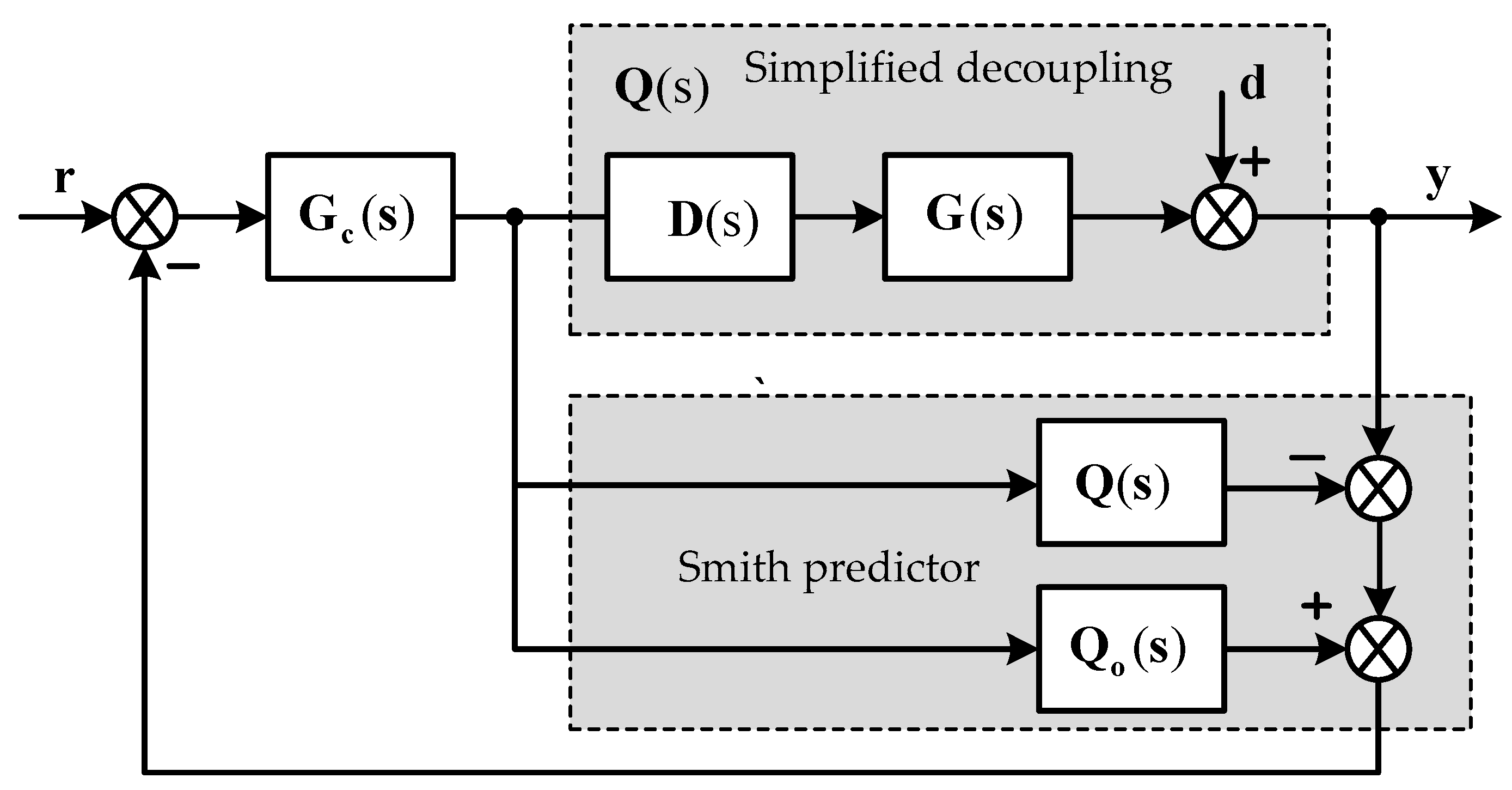
In this work, the controller structure called simplified decoupling Smith predictor (SDSP) [15] is used to deal with the main issues of multivariable processes including interactions between process variables and multiple delay times. The whole structure of the controller is shown in Figure 1.

In the Figure 1, G(s), D(s), Q(s) are the transfer function matrix, the decoupling matrix and the decoupled matrix of a TITO process, respectively. Due to the properties of the simplified decoupling, they have the forms as following:

$$\mathbf{G}(s)=\left[\begin{array}{cc}{g}_{11}(s)& g_{12}(s)\\ g_{21}(s)& g_{22}(s)\end{array}\right]; \mathbf{D}(s)=\left[\begin{array}{cc}1& d_{12}(s)\\ d_{21}(s)& 1\end{array}\right]; \mathbf{Q}(s)=\left[\begin{array}{cc}{q}_{11}(s)& 0\\ 0& q_{22}(s)\end{array}\right]$$

(9)

where the elements of D(s) and Q(s) can be calculated as shown in (10)–(12) [15]:

$$d_{12}(s)=-\frac{g_{12}(s)}{g_{11}(s)}; d_{21}(s)=-\frac{g_{21}(s)}{g_{22}(s)}$$

(10)

$$q_{11}(s)=g_{11}(s)-\frac{g_{12}(s)g_{21}(s)}{g_{22}(s)}$$

(11)

$$q_{22}(s)=g_{22}(s)-\frac{g_{12}(s)g_{21}(s)}{g_{11}(s)}$$

(12)

Various methods were proposed to approximate the diagonal elements of the decoupled matrix (q₁₁, q₂₂) to some standard forms [15,16,18,20,21]. However, all of them only deal with integer order transfer functions. In this work, a fractional order transfer function (FOTF) is employed to be the equivalent transfer function of Equations (11) and (12). The general form of the FOTF is as follows:

$$g_m(s)=\frac{K{e}^{-\theta s}}{{\tau }_2{s}^{{\alpha }_2}+{\tau }_1{s}^{{\alpha }_1}+1}\hspace{1em}\hspace{1em}\left(0<{\alpha }_1\le 1<{\alpha }_2<2\right)$$

(13)

where ${\tau }_1,{\tau }_2$ are time constants; $K$ is a gain; ${\alpha }_2,{\alpha }_1$ are fractional orders, assuming $0<{\alpha }_1\le 1<{\alpha }_2<2$; $\theta$ is a delay time.

In special case, when ${\tau }_2=0$, Equation (13) will become a simpler form:

$$g_m(s)=\frac{K{e}^{-\theta s}}{\tau s^{\alpha }+1}\hspace{1em}\hspace{1em}\left(0<\alpha <1\right)$$

(14)

In order to facilitate the approximation procedure, the parameter $\theta$ is a priori value that could be determined by the unit step response of the original model. Therefore, the number of tuning parameters will be written in the vector form as follow:

$$\mathbf{x}=\left[\begin{array}{ccccc}K& {\tau }_2& {\tau }_1& {\alpha }_2& {\alpha }_1\end{array}\right]$$

(15)

The different constraints of these parameters are given in (16):

$$\{\begin{array}{c}{K}_{\min }<K<K_{\max }\hfill \\ 0<{\tau }_1<{\tau }_{\max }\hfill \\ 0\le {\tau }_2<{\tau }_{\max }\hfill \\ 0<{\alpha }_1\le 1\hfill \\ 1<{\alpha }_2<2\hfill \end{array}$$

(16)

where $K_{\min },K_{\max },{\tau }_{\max }$ are determined based on the open-loop unit step responses of the original model.

The approximation technique using the PSO algorithm proposed by Chuong et al. [15] is addressed to find out the parameters in (15). Note that, from the condition (16), only ${\tau }_2$ can be equal to zero; and if happened, the reduced model becomes the simpler form as (14). Therefore, the approximated transfer function normally has one of the following forms:

$${\overline{q}}_i(s)=\frac{K_i{e}^{-{\theta }_{i}s}}{{\tau }_{2i}{s}^{{\alpha }_{2i}}+{\tau }_{1i}{s}^{{\alpha }_{1i}}+1}\hspace{1em}\hspace{1em}\left(0<{\alpha }_{1i}\le 1<{\alpha }_{2i}<2, i=1÷2\right)$$

(17)

$${\overline{q}}_i(s)=\frac{K_i{e}^{-{\theta }_{i}s}}{{\tau }_i{s}^{{\alpha }_i}+1}\hspace{1em}\hspace{1em}\left(0<{\alpha }_i<1, i=1÷2\right)$$

(18)

where ${\overline{q}}_i(s)$ is the equivalent transfer function of q_ii in Equations (11) and (12).

It is obvious that the delays still exist in the diagonal elements of the decoupled matrix and that make sluggish responses in the outputs [15,22]. However, because of the effect of the Smith predictors in the controller structure, the delay terms are eliminated from the closed loop functions. Consequently, ${\theta }_i$ is removed from Equations (17)–(18) and the following equations should be used to design controllers:

$${\overline{q}}_{io}(s)=\frac{K_i}{{\tau }_{2i}{s}^{{\alpha }_{2i}}+{\tau }_{1i}{s}^{{\alpha }_{1i}}+1}\hspace{1em}\hspace{1em}\left(0<{\alpha }_{1i}\le 1<{\alpha }_{2i}<2, i=1÷2\right)$$

(19)

$${\overline{q}}_{io}(s)=\frac{K_i}{{\tau }_i{s}^{{\alpha }_i}+1}\hspace{1em}\hspace{1em}\left(0<{\alpha }_i<1, i=1÷2\right)$$

(20)

where ${\overline{q}}_{io}(s)$ is the delay-free part of ${\overline{q}}_i(s)$.

2.3. IMC-Fractional PI/PID Controller Design

By using the controller structure as mentioned above, the multivariable processes become multi-loop systems. For each loop, a corresponding controller needs to be designed to meet the requirements of its closed loop responses. In this study, a new structure of a fractional PID controller is proposed for each loop, called I^σPI^λD^μ. In the case of the higher order process, Equation (19), a first order filter is also employed to improve its performances. Let the primary controller of each loop be as Equation (21):

$$g_{ci}(s)=K_{ci}\frac{1}{s^{{\sigma }_i}}\left(1+\frac{1}{{\tau }_{Ii}{s}^{{\lambda }_i}}+{\tau }_{Di}{s}^{{\mu }_i}\right)F_i(s)$$

(21)

where $K_{ci},{\tau }_{Ii}$ and ${\tau }_{Di}$ are proportional gain, integral time and derivative time respectively; ${\lambda }_i,{\mu }_i$ are fractional order of the integral and derivative terms; ${\sigma }_i$ is the fractional order of the ideal integral and ${\sigma }_i=1-{\lambda }_i$, in special case, when ${\lambda }_i=1$ (integral term with integer order) then ${\sigma }_i$ equals to zero; F_i(s) is the first order filter, $F_i(s)=\frac{1}{{\tau }_{Fi}s+1}$ where ${\tau }_{Fi}$ is a time constant.

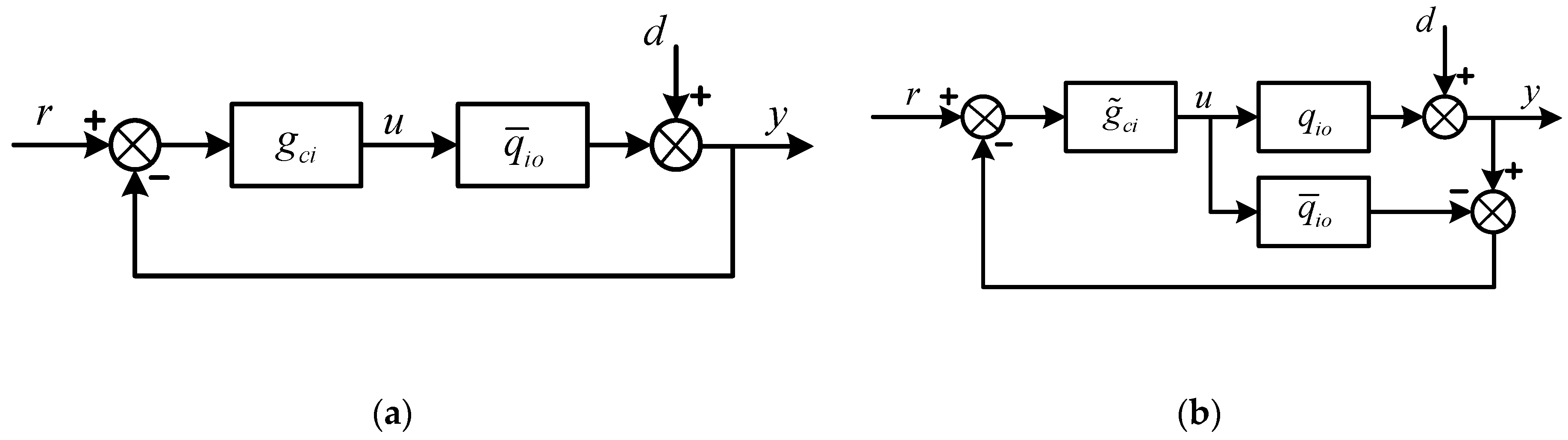
The IMC based PID procedure normally used for integer order processes is also addressed to design the proposed controller, I^σPI^λD^μ, for fractional order processes. Figure 2a,b show block diagrams of feedback control strategies including the classical feedback control and the internal model control as well [10,11,12,13,23]. Note that, in this case, the controlled process is a fractional order transfer function without delay time.

According to the IMC theory, the process model is divided into two parts:

$${\overline{q}}_{io}(s)=p_M(s)p_A(s)$$

(22)

where $p_A(s)$ contains delay time terms and/or RHP zeros and $p_A(0)=1$. According to Equations (19) and (20), $p_A(s)=1$.

Generally, the IMC controller is designed as

$${\tilde{g}}_{ci}(s)=p_M{}^{-1}(s)f_i$$

(23)

The term $f$ is called the IMC filter and normally has the form as follow:

$$f_i=\frac{1}{{\left({\tau }_{ci}s+1\right)}^{r_i}}$$

(24)

where ${\tau }_{ci}$ is an adjustable parameter which controls the tradeoff between the performance and robustness; $r_i$ is relative order and to be selected large enough to make the IMC controller (semi-) proper. Substituting Equation (24) into Equation (23):

$${\tilde{g}}_{ci}(s)=p_M{}^{-1}(s)\frac{1}{{\left({\tau }_{ci}s+1\right)}^{r_i}}$$

(25)

Therefore, the ideal feedback controller for achieving the desired loop responses can be easily obtained by:

$$g_{ci}(s)=\frac{{\tilde{g}}_{ci}(s)}{1-{\overline{q}}_{io}(s){\tilde{g}}_{ci}(s)}=\frac{p_M{}^{-1}(s)}{{\left({\tau }_{ci}s+1\right)}^{r_i}-p_A(s)}=\frac{p_M{}^{-1}(s)}{{\left({\tau }_{ci}s+1\right)}^{r_i}-1}$$

(26)

In this work, there are two cases of a process model to be considered:

Case 1: The fractional first order system:

$${\overline{q}}_{io}(s)=\frac{K_i}{{\tau }_i{s}^{{\alpha }_i}+1}\hspace{1em}\hspace{1em}\left(0<{\alpha }_i<1\right)$$

(27)

The proposed IMC filter structure

$$f_i=\frac{1}{{\tau }_{ci}s+1}$$

(28)

The ideal feedback controller is derived by:

$$g_{ci}(s)=\frac{{\tau }_i{s}^{{\alpha }_i}+1}{K_i{\tau }_{ci}s}=\frac{{\tau }_i}{K_i{\tau }_{ci}}\frac{1}{s^{1-{\alpha }_i}}\left(1+\frac{1}{{\tau }_i{s}^{{\alpha }_i}}\right)$$

(29)

Therefore, in this case, the proposed fractional controller settings are obtained:

$$K_{ci}=\frac{{\tau }_i}{K_i{\tau }_{ci}}; {\tau }_{Ii}={\tau }_i; {\lambda }_i={\alpha }_i; {\sigma }_i=1-{\alpha }_i; {\tau }_D{}_i={\tau }_{Fi}=0$$

(30)

Case 2: The fractional second order transfer function:

$${\overline{q}}_{io}(s)=\frac{K_i}{{\tau }_{2i}{s}^{{\alpha }_{2i}}+{\tau }_{1i}{s}^{{\alpha }_{1i}}+1}\hspace{1em}\hspace{1em}\left(0<{\alpha }_{1i}\le 1<{\alpha }_{2i}<2\right)$$

(31)

The proposed IMC filter structure

$$f_i=\frac{1}{{\left({\tau }_{ci}s+1\right)}^2}$$

(32)

The ideal feedback controller is obtained by:

$$g_{ci}(s)=\frac{{\tau }_{2i}{s}^{{\alpha }_{2i}}+{\tau }_{1i}{s}^{{\alpha }_{1i}}+1}{K_i{\tau }_{ci}s\left({\tau }_{ci}s+2\right)}$$

(33)

Rewritten Equation (35) into the form of Equation (21), the controller is derived as Equation (36):

$$g_{ci}(s)=\frac{{\tau }_{1i}}{2K_i{\tau }_{ci}}\frac{1}{s^{1-{\alpha }_{1i}}}\left(1+\frac{1}{{\tau }_{1i}{s}^{{\alpha }_{1i}}}+\frac{{\tau }_{2i}}{{\tau }_{1i}}{s}^{{\alpha }_{2i}-{\alpha }_{1i}}\right)\frac{1}{({\tau }_{ci}/2)s+1}$$

(34)

$$K_{ci}=\frac{{\tau }_{1i}}{2K_i{\tau }_{ci}}; {\tau }_{Ii}={\tau }_{1i}; {\tau }_{Di}=\frac{{\tau }_{2i}}{{\tau }_{1i}}; {\lambda }_i={\alpha }_{1i}; {\mu }_i={\alpha }_{2i}-{\alpha }_{1i}; {\sigma }_i=1-{\alpha }_{1i}; {\tau }_{Fi}=\frac{{\tau }_{ci}}{2}$$

(35)

The tuning rules for different types of process models are summarized in the

Table 1. Tuning rules for different types of fractional order process models.

Models	Tuning Rules
${\overline{q}}_{io}(s)=\frac{K_i}{{\tau }_i{s}^{{\alpha }_i}+1}$ $\left(0<{\alpha }_i<1\right)$	$K_{ci}=\frac{{\tau }_i}{K_i{\tau }_{ci}}$; ${\tau }_{Ii}={\tau }_i$; ${\lambda }_i={\alpha }_i$; ${\sigma }_i=1-{\alpha }_i$; ${\tau }_{Di}={\tau }_{Fi}=0$
${\overline{q}}_{io}(s)=\frac{K_i}{{\tau }_{2i}{s}^{{\alpha }_{2i}}+{\tau }_{1i}{s}^{{\alpha }_{1i}}+1}$ $\left(0<{\alpha }_{1i}\le 1<{\alpha }_{2i}<2\right)$	$K_{ci}=\frac{{\tau }_{1i}}{2K_i{\tau }_{ci}}$; ${\tau }_{Ii}={\tau }_{1i}$;${\tau }_{Di}=\frac{{\tau }_{2i}}{{\tau }_{1i}}$ ${\lambda }_i={\alpha }_{1i}$; ${\mu }_i={\alpha }_{2i}-{\alpha }_{1i}$;${\sigma }_i=1-{\alpha }_{1i}$ ${\tau }_{Fi}=\frac{{\tau }_{ci}}{2}$

.

2.4. System Performance and Robustness Analysis

2.4.1. Integral Absolute Error Index

To evaluate the closed-loop performance, the integral absolute error (IAE) criterion is considered, which is defined as

$$IAE={\displaystyle {\int }_0^T\left|e(t)\right|dt}$$

(36)

where $T$ is the simulation time.

2.4.2. Integral of Time-Weighted Absolute Error (ITAE)

Another performance index is also used to evaluate the response where t (time) is considered as a weighted coefficient of the absolute error. It is defined as follow:

$$ITAE={\displaystyle {\int }_0^{T}t\left|e(t)\right|dt}$$

(37)

2.4.3. Total Variation (TV)

To evaluate the magnitude of the manipulated input usage, the total up and down movement of the control signal is considered as.

$$TV={\displaystyle \sum _{k=1}^T\left|u(k+1)-u(k)\right|}$$

(38)

TV is normally used to measure the smoothness of manipulated variables and should be as small as possible.

2.4.4. Robust Stability Analysis

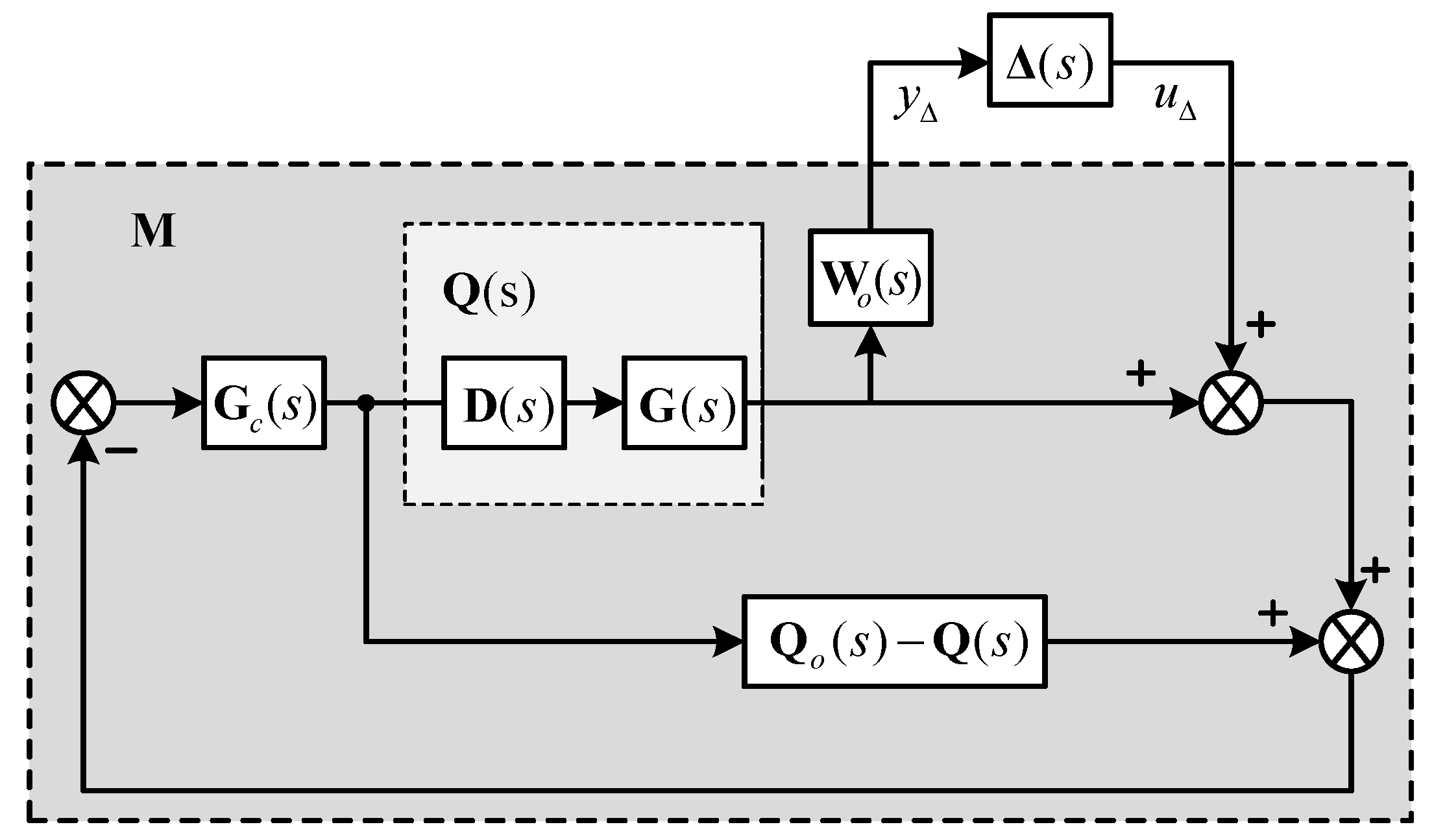
Robust stability is a very important criterion when evaluating the performance of a control system. Since the models used for analyzing and designing are normally imperfect matches with the real processes due to many sources of uncertainties. For fractional order control systems, in previous works, most authors focus exclusively on two criteria including maximum sensitivity (M_s) and maximum peak (M_p) in the frequency domain. In this study, the structured singular value (SSV) or μ-synthesis with the M-Δ structure, which is usually employed to evaluate the robustness of integer order systems, is also adopted to analyze the robust stability of the fractional order control systems. In addition, perturbations due to the multiplicative output uncertainty in each loop of multivariable processes are also considered as Figure 3.

The transfer function matrix from the outputs to the inputs of $\mathsf{\Delta }(s)$ can be easily obtained by:

$$\mathbf{M}(s)=-{\mathbf{W}}_o(s)\mathbf{Q}(s){\mathbf{G}}_c(s){\left[\mathbf{I}+{\mathbf{Q}}_o(s){\mathbf{G}}_c(s)\right]}^{-1}$$

(39)

where W_o(s) is a weighted matrix representing the output uncertainties.

According to the μ–synthesis, the control system will remain stable under multiplicative output uncertainty if the following constraint inequality is satisfied

$$\mu \left[\mathbf{M}(j\omega )\right]=\mu \left\{{\mathbf{W}}_{o}j\omega )\mathbf{Q}(j\omega ){\mathbf{G}}_c(j\omega ){\left[\mathbf{I}+{\mathbf{Q}}_o(j\omega ){\mathbf{G}}_c(j\omega )\right]}^{-1}\right\}<1,\hspace{1em}\hspace{0.17em}\forall \omega$$

(40)

Note that, in this work, Q(s), Q_o(s) and G_c(s) are in fractional order forms.

3. Results

In this section, three examples of the well-known TITO processes are considered to demonstrate the performances of the proposed method in comparison with those of other existing methods.

Example 1.

Heavy oil fractionator

It is a 2 × 2 process given in [20]. The open-loop transfer function matrix is as follow (43) where time constants and delays are expressed in minutes.

$$\mathbf{G}(s)=\left[\begin{array}{cc}\frac{4.05e^{-27s}}{27s+1}& \frac{1.77e^{-28s}}{60s+1}\\ \frac{5.39e^{-18s}}{50s+1}& \frac{5.72e^{-14s}}{60s+1}\end{array}\right]$$

(41)

The decoupler matrix is easily obtained using the Equation (10) and the result is as follow:

$$\mathbf{D}(s)=\left[\begin{array}{cc}1& -\frac{0.437(27s+1)}{60s+1}{e}^{-s}\\ \frac{0.9423(60s+1)}{(50s+1)}{e}^{-4s}& 1\end{array}\right]$$

(42)

Then, using (11) and (12) to calculate the diagonal elements of the decoupled matrix. However, in this case, the approximation technique using the PSO algorithm [15] is addressed to derive the fractional order transfer functions. The results are obtained by the following equations:

$$q_{11}=\frac{2.3979e^{-27s}}{15.1333s^{1.1334}+6.9815s+1}$$

(43)

$$q_{22}=\frac{3.3877e^{-14s}}{45.6092s^{0.9967}+1}$$

(44)

Using the above fractional transfer functions and the proposed controller for each case, the fractional controllers are derived as follows:

$$g_{c1}=0.0622\left(1+\frac{1}{4.166s}+5.7077s^{0.1334}\right)\frac{1}{7s+1}$$

(45)

$$g_{c2}=0.6732\frac{1}{s^{0.0033}}\left(1+\frac{1}{45.6092s^{0.9967}}\right)$$

(46)

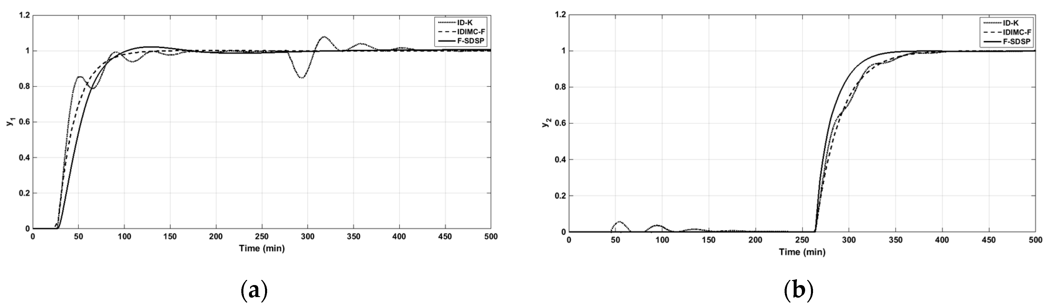
In this example, the proposed method is compared with those of inverted decoupling internal model control with filter (IDIMC-F) and centralized inverted decoupling control (ID-K) which are proposed by Garrido [20]. The closed-loop responses for the sequential step changes in the set-points of loops 1 and 2 are shown in Figure 4a,b. The performance indices of the three methods are summarized in

Table 2. The resulting performance indices for Example 1.

Tuning Method	IAE	ITAE	TV	$\mathit{\mu }[\mathbf{M}]$
F-SDSP	57.824	10173	1.4838	0.200
IDIMC-F	750.00	218750	1.7289	0.7068
ID-K	95.521	14561	14.678	0.3880

.

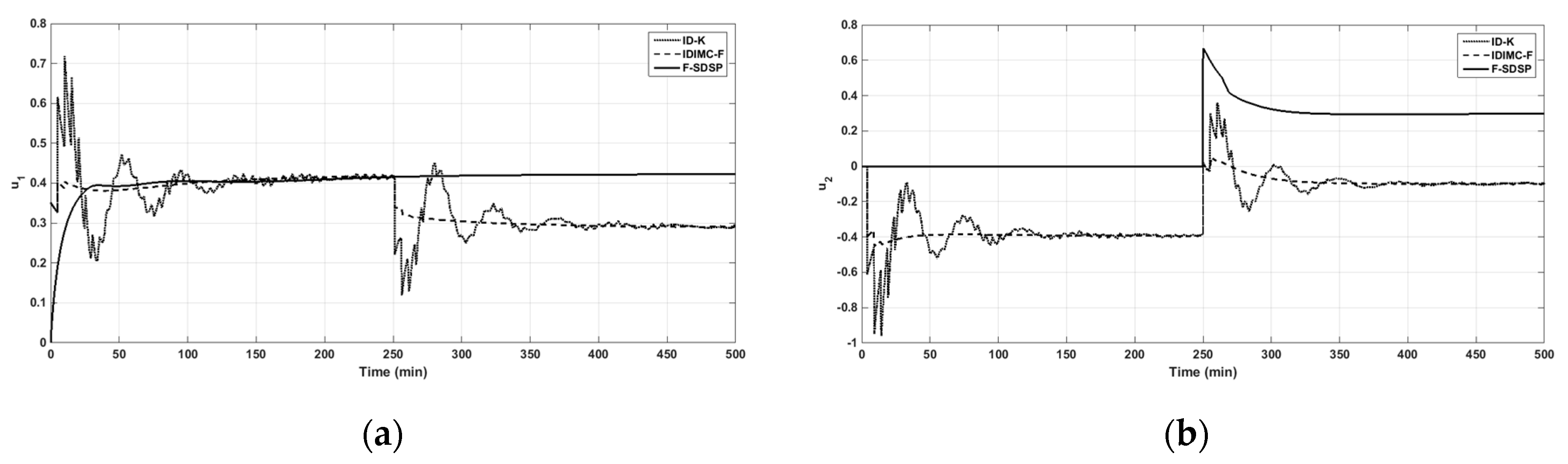
From Figure 4a,b, it can be seen that the proposed controller has familiar response compared to the IDIMC-F method and far better than the ID-K one in loop 1, however, in loop 2 the proposed method has faster rising time and shorter settling time in comparison with the others. Disturbance rejection performance by considering the mutual effects of sequential changes on loops 1 and 2 is much improved in the proposed method. As a result, the performance indices including TV, IAE, and ITAE of the proposed one are superior to the others. Figure 5a,b illustrate the manipulated variables of both loops with respect to time and they indicate that the proposed method has smoother signals.

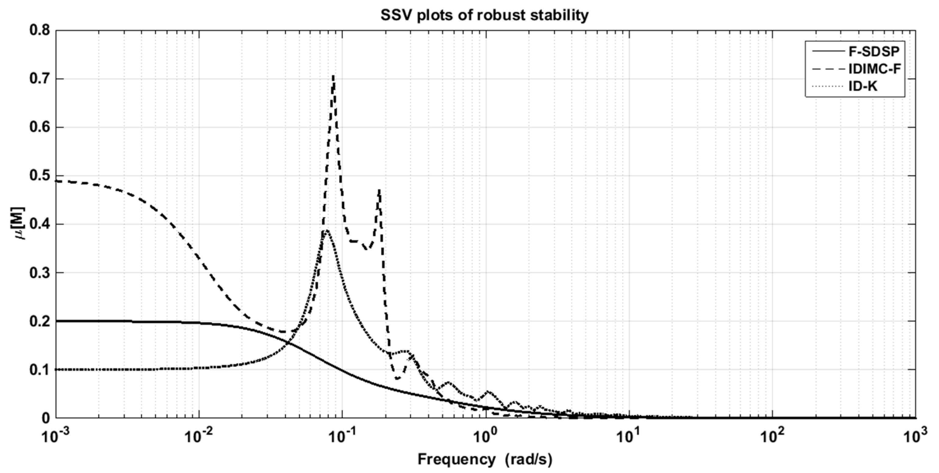
The robust stability of the system is investigated using Equation (42) with a multiplicative output uncertainty, where ${\mathbf{W}}_o(s)=diag\left\{-\frac{s+0.2}{2s+1},-\frac{s+0.2}{2s+1}\right\}$ which means that relative uncertainties are decreased by 50% in a high frequency range and by 20% at low frequencies. Figure 6 presents the performances of stability analysis of the proposed method along with the others. It is obvious that the proposed method guarantees the robustness of the control system in the whole range of frequency. The maximum values of μ listed in Table 2 show the smallest value that belongs to the proposed method.

Example 2.

Wood and Berry (WB) distillation column

The well-known WB column is used for evaluating the performances of the proposed method. The transfer function matrix of WB can be found in [24] and expressed as Equation (49):

$$\mathbf{G}(s)=\left[\begin{array}{cc}\frac{12.8e^{-s}}{16.7s+1}& \frac{-18.9e^{-3s}}{21s+1}\\ \frac{6.6e^{-7s}}{10.9s+1}& \frac{-19.4e^{-3s}}{14.4s+1}\end{array}\right]$$

(47)

The matrix of the simplifier decoupler for this process can be obtained by Equation (10):

$$\mathbf{D}(s)=\left[\begin{array}{cc}1& \frac{1.477(16.7s+1)e^{-2s}}{21s+1}\\ \frac{0.34(14.4s+1)e^{-4s}}{10.9s+1}& 1\end{array}\right]$$

(48)

Similar to the Example 1, the FOTFs of the diagonal elements of decoupled matrix are approximated as follows:

$$q_{11}=\frac{6.4911e^{-s}}{7.1079s^{0.8714}+1}$$

(49)

$$q_{22}=\frac{-9.8693e^{-3s}}{3.3615s^{1.788}+5.2645s^{0.8462}+1}$$

(50)

According to Table 1, the proposed fractional controllers are obtained for each loop:

$$g_{c1}=0.2882\frac{1}{s^{0.1286}}\left(1+\frac{1}{7.1079s^{0.8714}}\right)$$

(51)

$$g_{c2}=-0.1212\frac{1}{s^{0.1538}}\left(1+\frac{1}{5.2645s^{0.8462}}+0.6385s^{0.9418}\right)\frac{1}{1.1s+1}$$

(52)

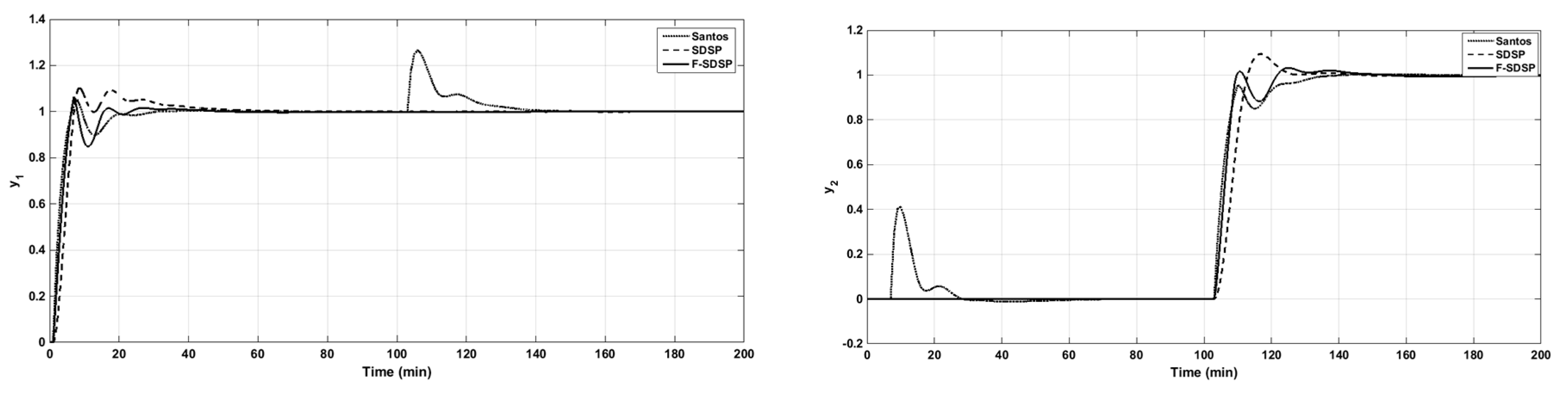
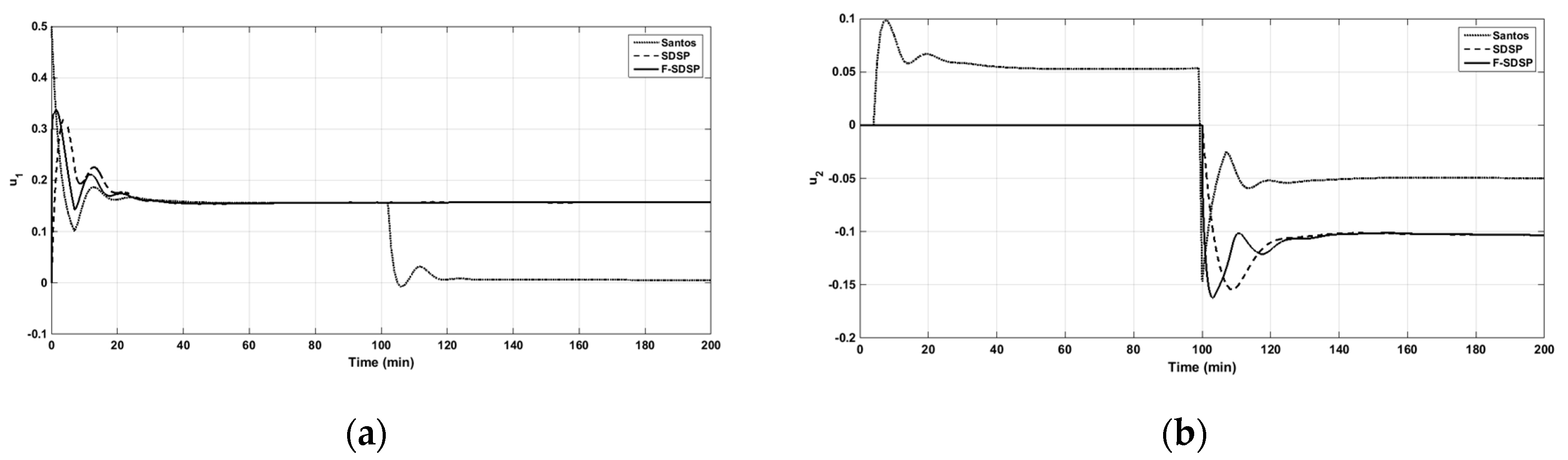
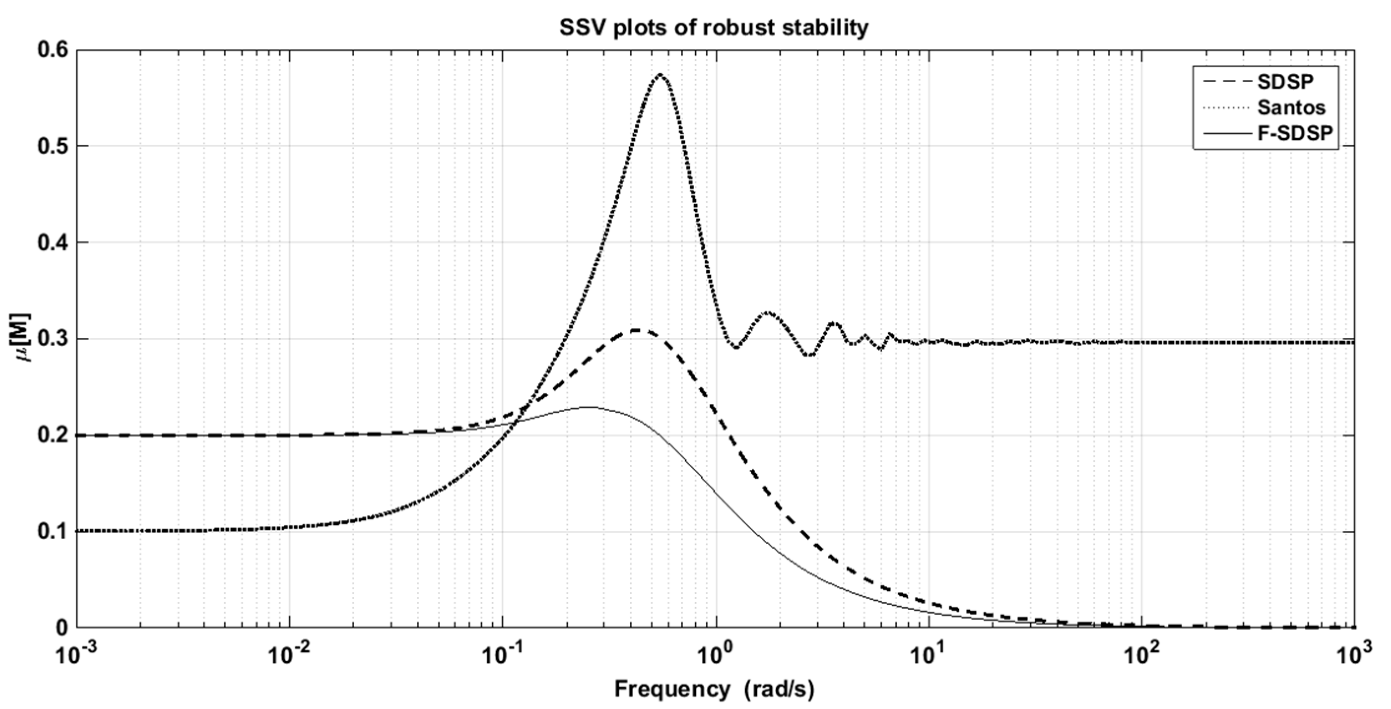
The performances of the proposed method are compared with those of the previous works including the simplified decoupling Smith predictor (SDSP) [15] and simplified filter Smith predictor proposed by Santos et al. [22]. The sequential unit step changes in the set-points are made to the 1st and 2nd loop at t = 0 (min) and t = 100 (min), respectively. The closed-loop responses to the set-point changes, the control signals of loop 1 and 2 are shown in Figure 7a,b and Figure 8a,b, respectively. The performance indices are summarized in

Table 3. The performance indices for the wood and berry (WB) column.

Tuning Method	IAE	ITAE	TV	$\mathit{\mu }[\mathbf{M}]$
F-SDSP	9.221	631.207	0.9587	0.2291
SDSP	10.963	667.088	0.7720	0.3091
Santos	13.294	881.098	1.2976	0.5750

. From the figures, it is obvious that the F-SDSP and SDSP methods have almost the same performance. However, when considering Table 3, the proposed method still gives better performance indices. In comparison with the Santos’ approach, the F-SDSP has far better responses in both set-point changes and disturbance rejection.

The robustness analysis of those methods is illustrated in Figure 9. In this case, the uncertainties of 10% of gains are applied to the Santos approach while the other approaches still keep the same uncertainties as the previous example, i.e. the uncertainties are decreased by 50% at high frequencies and increased by 20% in a low-frequency range. The maximum μ values shown in Table 3 prove that the proposed controller has the smallest value that means the best robustness among those approaches.

Example 3.

Vinante and Luyben (VL) column

The transfer function matrix for a VL column introduced by Luyben [25] has the following form:

$$\mathbf{G}(s)=\left[\begin{array}{cc}\frac{-2.2e^{-s}}{7s+1}& \frac{1.3e^{-0.3s}}{7s+1}\\ \frac{-2.8e^{-1.8s}}{9.5s+1}& \frac{4.3e^{-0.35s}}{9.2s+1}\end{array}\right]$$

(53)

The simplified decoupling matrix can be easily obtained by using Equation (10):

$$\mathbf{D}(s)=\left[\begin{array}{cc}1& 0.591\\ \frac{0.651(9.2s+1)e^{-1.45s}}{9.5s+1}& 1\end{array}\right]$$

(54)

Similar to the previous examples, the diagonal elements q₁₁ and q₂₂ are approximated to the fractional forms as Equation (17) or (18). The obtained results are as the following equations:

$$q_{11}=\frac{-1.3629e^{-s}}{6.6757s^{0.97}+1}$$

(55)

$$q_{22}=\frac{2.6679e^{-0.3s}}{8.8871s^{0.9683}+1}$$

(56)

In this example, the fractional controllers are obtained as follows:

$$g_{c1}=-2.5765\frac{1}{s^{0.03}}\left(1+\frac{1}{6.6757s^{0.97}}\right)$$

(57)

$$g_{c2}=2.082\frac{1}{s^{0.0317}}\left(1+\frac{1}{8.8871s^{0.9683}}\right)$$

(58)

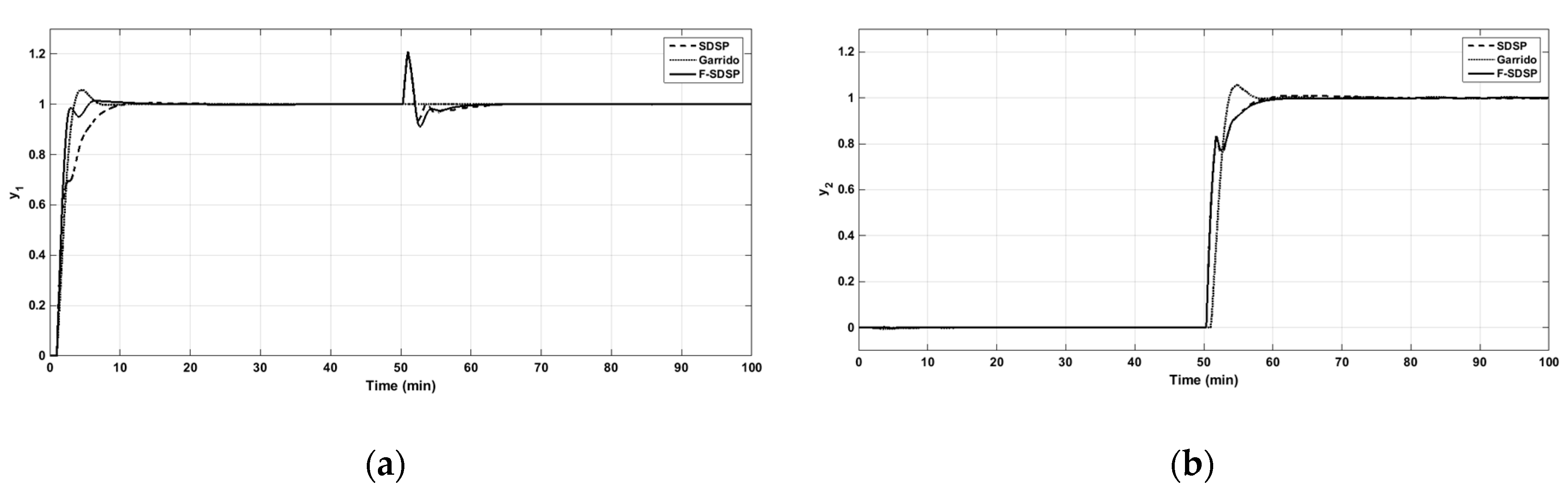
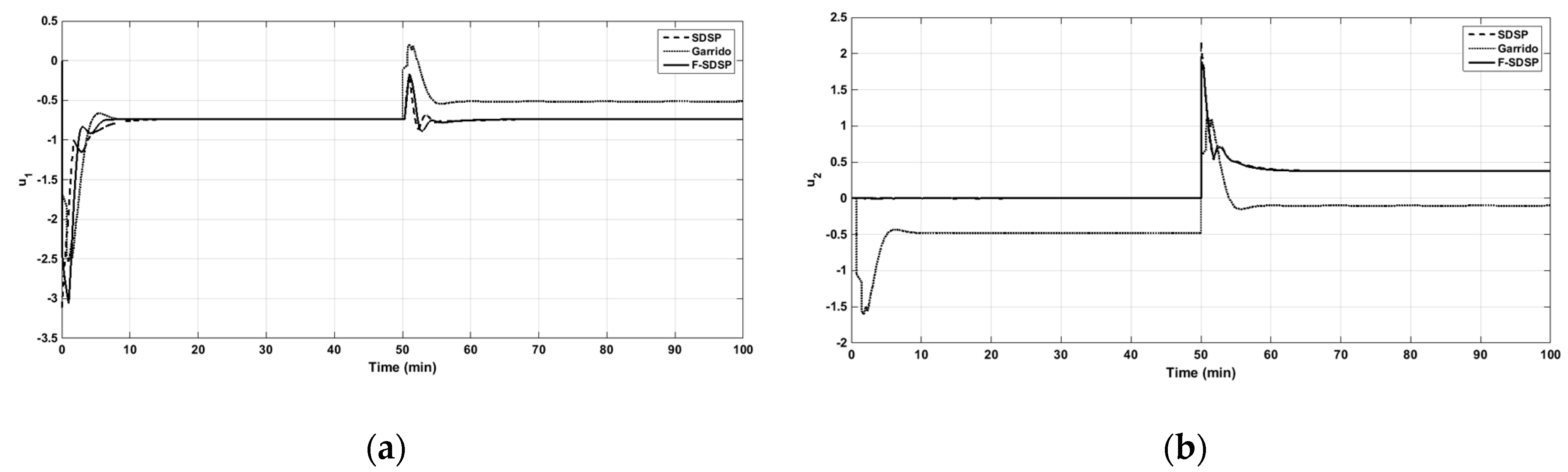
In this simulation, the performances of the proposed method are compared with those of the simplified decoupling Smith predictor (SDSP [15]) and the centralized inverted decoupling method (Garrido et al. [21]). For the sequential unit step changes in the set-points, Figure 10a,b compare the closed-loop time responses afforded by the proposed and other methods. It is clear that in the 1st loop, the fractional controller shows superior responses over the others in a set-point change. In the 2nd loop, the obtained performance is almost the same as SDSP one (dash line) and still better than the response of the centralized inverted decoupling proposed by Garrido (dot line). The control signals of the two loops are shown in Figure 11a,b. Moreover, the values of the performance indices in

Table 4. The performance indices in the Example 3.

Tuning Method	IAE	ITAE	TV	$\mathit{\mu }[\mathbf{M}]$
F-SDSP	3.7490	101.66	10.838	0.2974
SDSP	3.4382	102.83	8.7549	0.3046
Garrido	4.5255	126.04	11.295	0.4107

also confirm the obtained results.

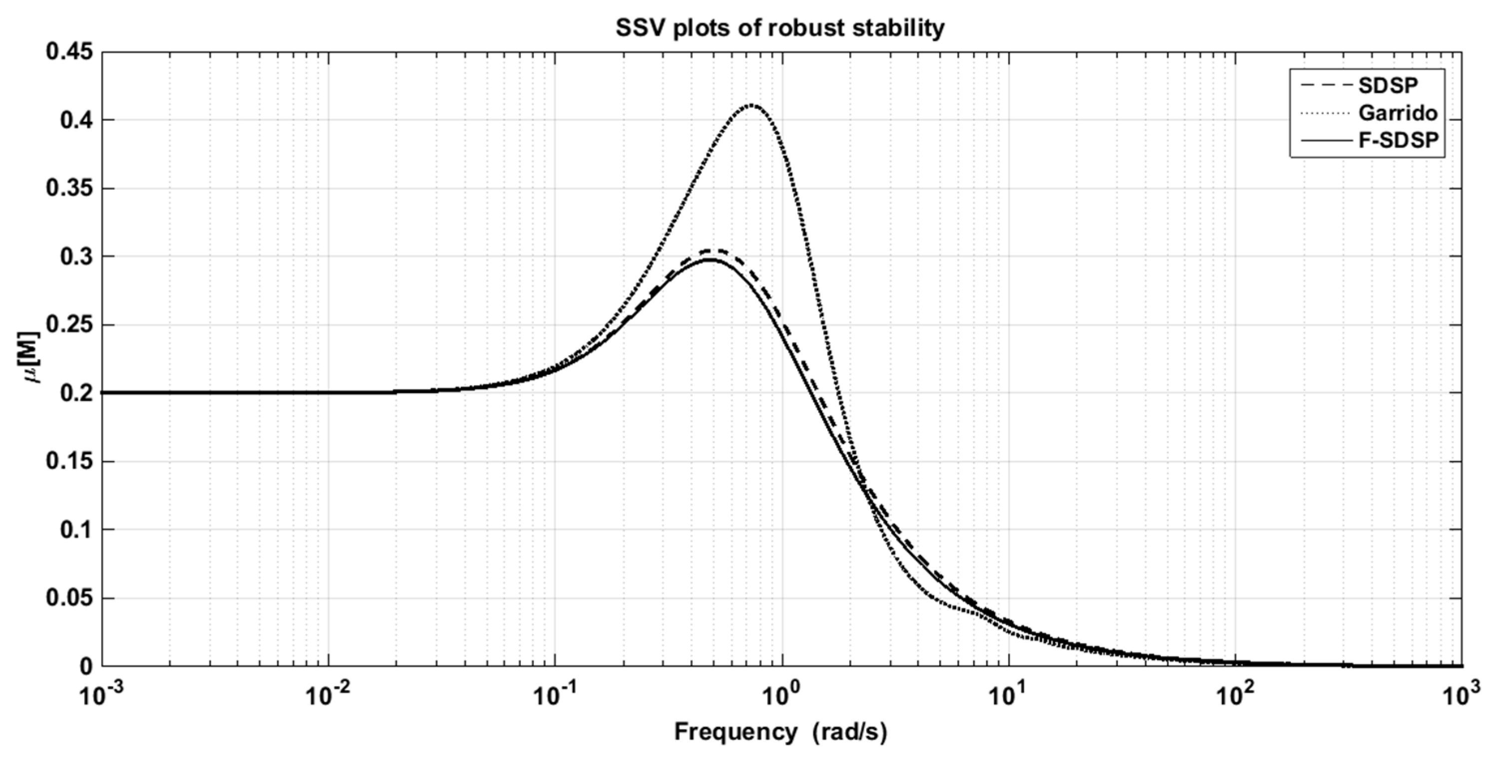
The robustness analysis in this example is illustrated in Figure 12 in which the weighted matrix, Wo(s), is the same as previous examples. The figure shows that the proposed method and the SDSP controller have similar robustness. On the other hand, in comparison with Garrido’s method, the proposed F-SDSP presents much better robustness performance. The μ values of those methods are also listed in Table 4 in which the fractional controller gives the smallest value.

4. Conclusions

In this paper, a new formula of fractional PID controller is proposed to apply for a two-input two-output process. In order to deal with the issues of multivariable systems including interactions between process variables and multiple delay times, the simplified decoupling Smith predictor structure proposed by Chuong et al. is addressed. However, it is different from the previous work, the fractional order process is adopted to approximate the complicated elements of a decoupled matrix. The analytical tuning rules of the proposed fractional PI/PID controllers are also derived for the delay-free parts of the approximated fractional transfer functions. The effectiveness and robustness of the proposed controller are proved by applying to some well-known TITO processes. In general, the obtained results demonstrate the better performances of the proposed controller in both set-point changes as well as load disturbances. The robust stability is always guaranteed with the smallest μ values compared to other methods.

References

- Podlubny, I. Fractional-Order Systems and PIλDμ-Controllers. IEEE Trans. Autom. Control 1999, 44, 208–214. [Google Scholar] [CrossRef]
- Chen, Y.; Bhaskaran, T.; Xue, D. Practical Tuning Rule Development for Fractional Order Proportional and Integral Controllers. J. Comput. Nonlinear Dyn. 2008, 3, 021403. [Google Scholar] [CrossRef] [Green Version]
- Monje, C.A.; Chen, Y.; Vinagre, B.M.; Xue, D.; Feliu-Batlle, V. Fractional-Order Systems and Controls, Fundamentals and Applications; Springer: London, UK, 2010. [Google Scholar]
- Rabah, K.; Ladaci, S.; Lashab, M. Bifurcation-based Fractional Order PIλ Dμ Controller Design Approach for Nonlinear Chaotic Systems. Front. Inf. Technol. Electron. Eng. 2018, 19, 180–191. [Google Scholar] [CrossRef]
- Luo, Y.; Chen, Y.Q.; Wang, C.Y.; Pi, Y.G. Tuning fractional order proportional integral controllers for fractional order systems. J. Process Control 2010, 20, 823–831. [Google Scholar] [CrossRef]
- Beschi, M.; Padula, F.; Visioli, A. Fractional robust PID control of a solar furnace. Control Eng. Pract. 2016, 60, 190–199. [Google Scholar] [CrossRef]
- De Keyser, R.; Muresan, C.I.; Ionescu, C.M. A novel auto-tuning method for fractional order PI/PD controllers. ISA Trans. 2016, 62, 268–275. [Google Scholar] [CrossRef]
- Padula, F.; Visioli, A. Tuning rules for optimal PID and fractional-order PID controllers. J. Process Control 2011, 21, 69–81. [Google Scholar] [CrossRef]
- Vu, T.N.; Lee, M. Analytical design of fractional-order proportional-integral controllers for time-delay processes. ISA Trans. 2013, 52, 583–591. [Google Scholar] [CrossRef]
- Vu, T.N.; Lee, M. Smith predictor based fractional-order PI control for time-delay processes. Korean J. Chem. Eng. 2014, 31, 1321–1329. [Google Scholar] [CrossRef]
- Li, D.; Liu, L.; Jin, Q.; Hirasawa, K. Maximum sensitivity based fractional IMC-PID controller design for non-integer order system with time delay. J. Process Control 2015, 31, 17–29. [Google Scholar] [CrossRef]
- Amoura, K.; Mansouri, R.; Bettayeb, M.; Al-Saggaf, U.M. Closed-loop step response for tuning PID-fractional-order-filter controllers. ISA Trans. 2016, 64, 247–257. [Google Scholar] [CrossRef]
- Li, M.; Zhou, P.; Zhao, Z.; Zhang, J. Two-degree-of-freedom fractional order-PID controllers design for fractional order processes with dead-time. ISA Trans. 2016, 61, 147–154. [Google Scholar] [CrossRef] [Green Version]
- Bouyedda, H.; Ladaci, S.; Sedraoui, M.; Lashab, M. Identification and Control design for a class of non-minimum Phase dead-time Systems based on fractional-order Smith Predictor and Genetic Algorithm Technique. Int. J. Dyn. Control 2019, 7, 914–925. [Google Scholar] [CrossRef]
- Chuong, V.L.; Vu, T.N.L.; Truong, N.T.N.; Jung, J.H. An Analytical Design of Simplified Decoupling Smith Predictors for Multivariable Processes. Appl. Sci. 2019, 9, 2487. [Google Scholar] [CrossRef] [Green Version]
- Garrido, J.; Vázquez, F.; Morilla, F. Centralized multivariable control by simplified decoupling. J. Process Control 2012, 22, 1044–1062. [Google Scholar] [CrossRef] [Green Version]
- Truong, N.L.V.; Lee, M. Independent design of multi-loop PI/PID controllers for interacting multivariable processes. J. Process Control 2010, 20, 922–933. [Google Scholar]
- Truong, N.L.V.; Lee, M. An extended method of simplified decoupling for multivariable processes with multiple time delays. J. Chem. Eng. Jpn. 2013, 46, 279–293. [Google Scholar]
- Skogestad, S.; Postlethwaithe, I. Multivariable Feedback Control Analysis and Design, 1st ed.; John Wiley & Sons: Hoboken, NJ, USA, 1996. [Google Scholar]
- Garrido, J.; Vázquez, F.; Morilla, F. Inverted decoupling internal model control for square stable multivariable time delay systems. J. Process Control 2014, 24, 1710–1719. [Google Scholar] [CrossRef] [Green Version]
- Garrido, J.; Vázquez, F.; Morilla, F. Centralized Inverted Decoupling Control. Ind. Eng. Chem. Res 2013, 52, 7854–7866. [Google Scholar] [CrossRef] [Green Version]
- Santos, T.L.; Torrico, B.C.; Normey-Rico, J.E. Simplified filtered Smith predictor for MIMO processes with multiple time delays. ISA Trans. 2016, 65, 339–349. [Google Scholar] [CrossRef]
- Morari, M.; Zafiriou, E. Robust Process Control; Prentice Hall: Englewood Cliffs, NJ, USA, 1989. [Google Scholar]
- Wood, R.K.; Berry, M.W. Terminal composition control of binary distillation column. Chem. Eng. Sci. 1973, 28, 1707–1717. [Google Scholar] [CrossRef]
- Luyben, W.L. Simple method for tuning SISO controllers in multivariable systems. Ind. Eng. Chem. Process Des. Dev. 1986, 25, 654–660. [Google Scholar] [CrossRef]
Figure 1.
The simplified decoupling Smith predictor (SDSP) structure with approximated fractional order processes (F-SDSP).
Figure 2.
The one degree of freedom feedback control diagram. (a) Classical feedback control (b) Internal model control.
Figure 3.
M-Δ structure with multiplicative output uncertainties.
Figure 4.
(a) Closed-loop responses to the unit step changes in the set-point of loop 1 in Example 1. (b) Closed-loop responses to the unit step changes in the set-point of loop 2 in Example 1.
Figure 5.
(a) The control signal of loop 1 in Example 1. (b) The control signal of loop 1 in Example 1.
Figure 6.
The structured singular value (SSV) plots of robust stability in Example 1.
Figure 7.
(a) Closed-loop responses to the unit step changes in the set-point of loop 1 in Example 2*. (b) Closed-loop responses to the unit step changes in the set-point of loop 2 in Example 2*. (* Santos in all Figure 7, Figure 8 and Figure 9 is used instead of “Simplified filter Smith predictor proposed by Santos et al. [22]”).
Figure 8.
(a) The control signal in loop 1 in Example 2*. (b) The control signal in loop 2 in Example 2*.
Figure 9.
The SSV plots of robust stability in Example 2*.
Figure 10.
(a) Closed-loop responses to the unit step changes in the set-point of loop 1 in Example 3*. (b) Closed-loop responses to the unit step changes in the set-point of loop 2 in Example 3*. (* Garrido in all Figure 10, Figure 11 and Figure 12 is used instead of “The centralized inverted decoupling method proposed by Garrido et al. [21]”).
Figure 11.
(a) The control signal of loop 1 in Example 3*. (b) The control signal of loop 2 in Example 3*.
Figure 12.
The SSV plots of robust stability in Example 3*.