Neural Computing Improvement Using Four Metaheuristic Optimizers in Bearing Capacity Analysis of Footings Settled on Two-Layer Soils

Abstract
:1. Introduction
2. Methodology
2.1. Artificial Neural Network
2.2. Hybrid Metaheuristic Algorithms
| Algorithm 1. The pseudo-code of the whale optimization algorithm (WOA) [53] |
| Initialize the whale population Xi (i = 1, 2, …, n) Calculate the fitness of each search agent X∗ the best search agent while (t < maximum number of iterations) for each search agent Update a, A, C, l, and P if1 (P < 0.5) if2 (|A| < 1) Update the position of the current search agent else if2 (|A| ≥ 1) Select a random search agent (Xrand) Update the position of the current search agent end if2 else if1 (P ≥ 0.5) Update the position of the current search agent end if1 end for Check if any search agent goes beyond the search space and amend it Calculate the fitness of each search agent Update X∗ if there is a better solution t = t + 1 end while return X∗ |
| Algorithm 2. The pseudo-code of the league champion optimization algorithm (LCA) [54] |
| Initialize the league size (L) and the number of seasons (S); t = 1; Generate a league schedule; Initialize team formations (generate a population of L solutions) and determine the playing strengths (function or fitness value) along with them. Let the initialization also be the team’s current best formation; While t < = S × (L − 1) Based on the league schedule at week t, determine the winner/loser among every pair of teams using a playing strength-based criterion; t = t + 1 For i = 1 to L Devise a new formation for team i for the forthcoming match, while taking into account the team’s current best formation and previous week events. Evaluate the playing strength of the resulting arrangement; If the new formation is the fittest one (that is, the new solution is the best solution achieved so far for the i-th member of the population), hereafter consider the new formation as the team’s current best formation; End For If mod (t, L−1) = 0 Generate a league schedule; End If End While |
| Algorithm 3. The pseudo-code of the moth–flame optimization (MFO) algorithm [55] |
| While iteration < max iteration Update flame number Obj = fitness function (Moths); if Iteration = 1 Sort the moths based on their objective functions; update the flames Iteration = 0; else Sort the moths based on their objective functions and flames from last iteration; update the flames end linearly decrease the convergence constant for j = 1: Number of moths for k = 1: Number of variables, update r and t Calculate the distance of moth from each flame; update the values of the variables of moth from the corresponding flame end end Iteration = iteration + 1; end |
| Algorithm 4. The pseudo-code of the ant colony optimization (ACO) algorithm [56] |
| Initialization: Algorithm parameters; Ant population size K; Maximum number of iteration NMax; Generation: Generating the pheromone matrix for the ant k; Update the pheromone values and set x* = k; i = 1; Repeat for k = 1 to K Compute the cost function for the ant k; Compute probability move of ant individual; if f(k) < f(x*) Then Update the pheromone values; Set x* = k; End if End for Until I > NMax; |
3. Data Collection
4. Results and Discussion
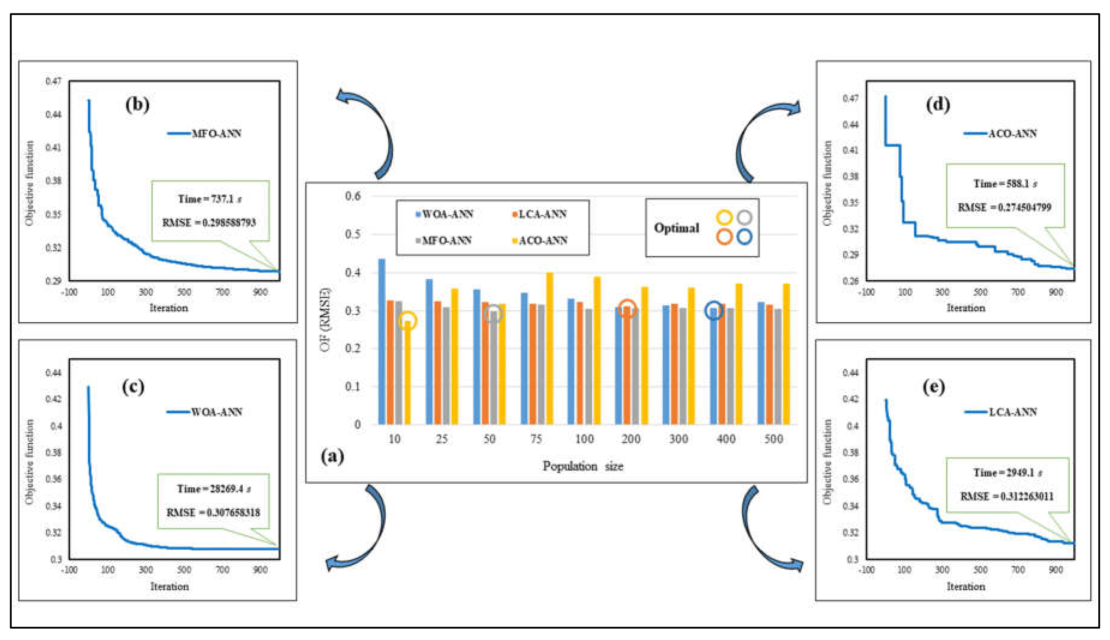
4.1. Hybridizing the ANN Using Metaheuristic Algorithms
4.2. Accuracy Assessment Criteria
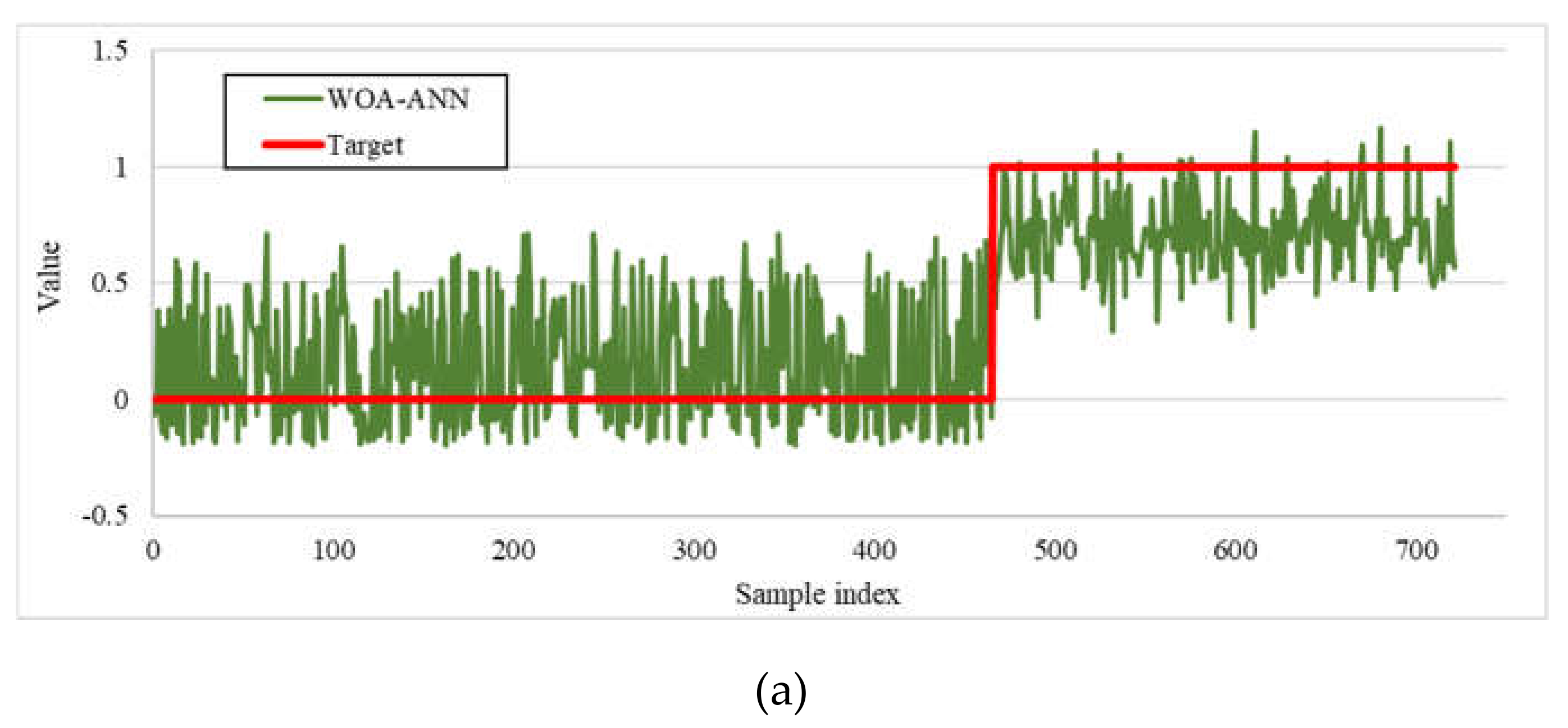
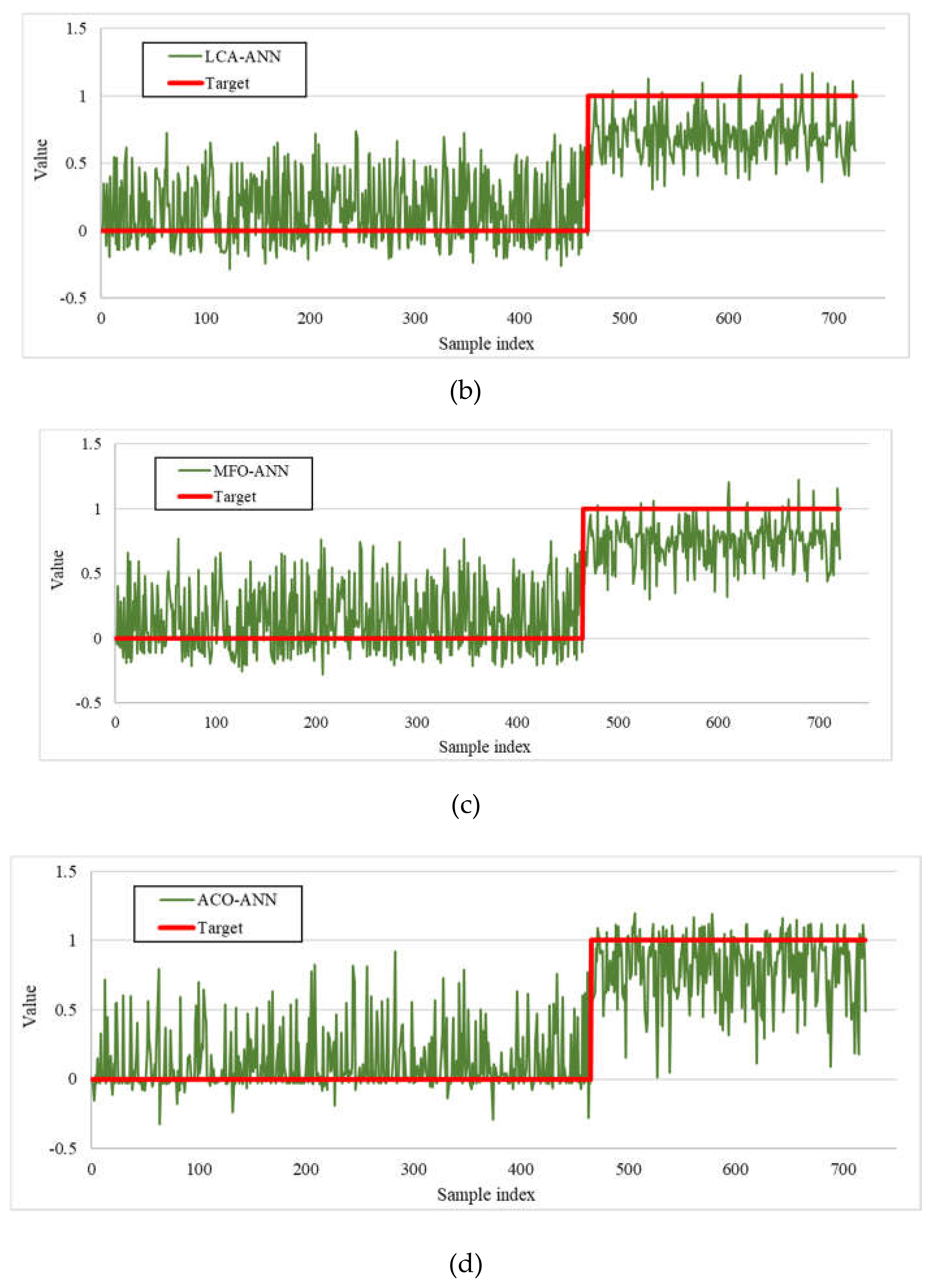
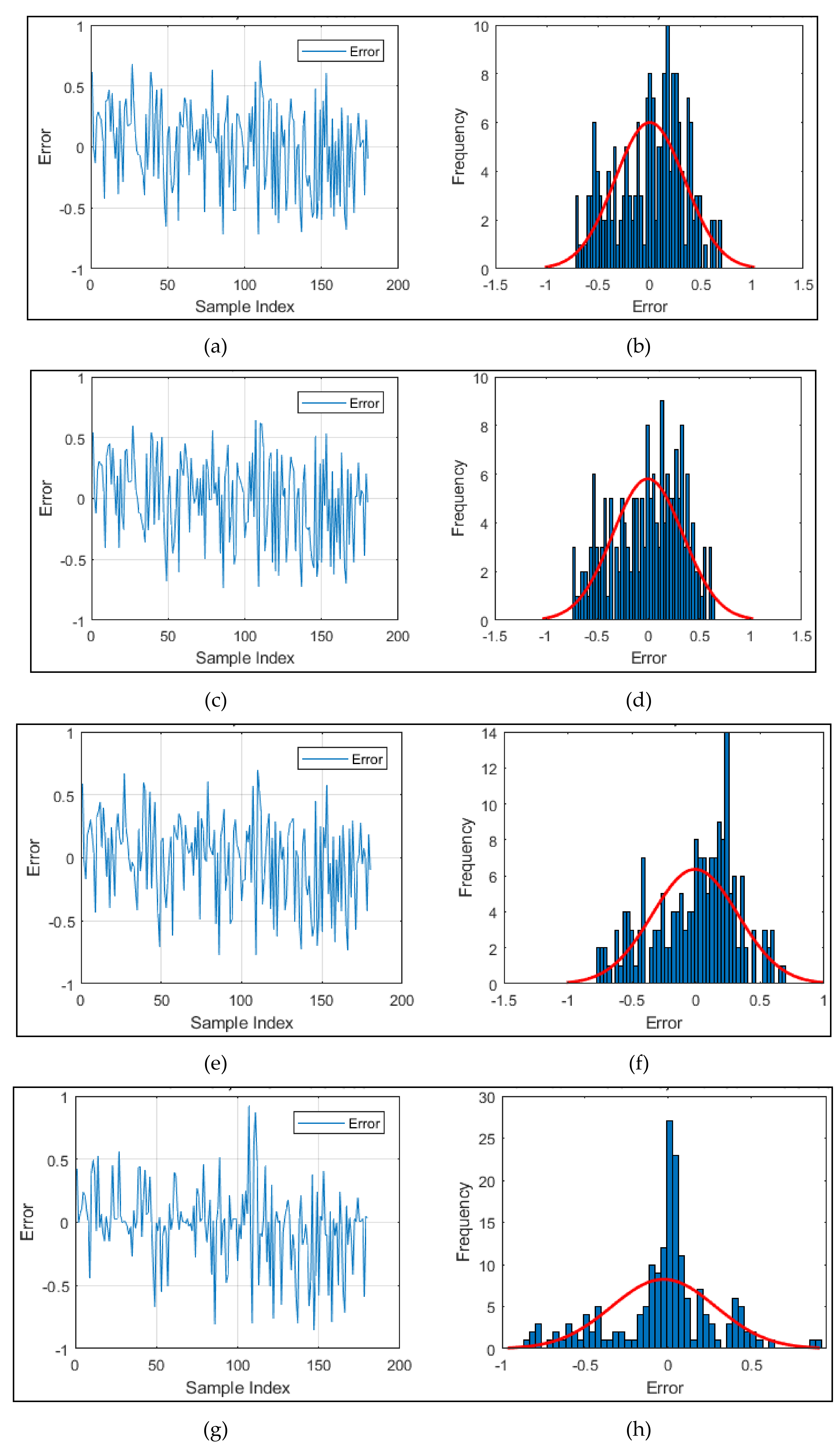
4.3. Accuracy Assessment of the Predictive Models
4.4. Presenting the Neural Predictive Formula
5. Conclusions
Author Contributions
Funding
Conflicts of Interest
References
- Momeni, E.; Nazir, R.; Armaghani, D.J.; Sohaie, H. Bearing capacity of precast thin-walled foundation in sand. Proc. Inst. Civ. Eng. Geotech. Eng. 2015, 168, 539–550. [Google Scholar] [CrossRef]
- Moayedi, H.; Moatamediyan, A.; Nguyen, H.; Bui, X.-N.; Bui, D.T.; Rashid, A.S.A. Prediction of ultimate bearing capacity through various novel evolutionary and neural network models. Eng. Comput. 2019, 35, 1–17. [Google Scholar] [CrossRef]
- Keskin, M.S.; Laman, M. Model studies of bearing capacity of strip footing on sand slope. Ksce J. Civ. Eng. 2013, 17, 699–711. [Google Scholar] [CrossRef]
- Das, B.M.; Sobhan, K. Principles of Geotechnical Engineering; Cengage Learning: Belmont, CA, USA, 2013. [Google Scholar]
- Ranjan, G.; Rao, A. Basic and Applied Soil Mechanics; New Age International: New Delhi, India, 2007. [Google Scholar]
- Meyerhof, G.; Hanna, A. Ultimate bearing capacity of foundations on layered soils under inclined load. Can. Geotech. J. 1978, 15, 565–572. [Google Scholar] [CrossRef]
- Terzaghi, K.; Peck, R.B.; Mesri, G. Soil Mechanics in Engineering Practice; John Wiley & Sons: Hoboken, NJ, USA, 1996. [Google Scholar]
- Lotfizadeh, M.R.; Kamalian, M. Estimating bearing capacity of strip footings over two-layered sandy soils using the characteristic lines method. Int. J. Civ. Eng. 2016, 14, 107–116. [Google Scholar] [CrossRef]
- Frydman, S.; Burd, H.J. Numerical studies of bearing-capacity factor N γ. J. Geotech. Geoenviron. Eng. 1997, 123, 20–29. [Google Scholar] [CrossRef]
- Florkiewicz, A. Upper bound to bearing capacity of layered soils. Can. Geotech. J. 1989, 26, 730–736. [Google Scholar] [CrossRef]
- Ghazavi, M.; Eghbali, A.H. A simple limit equilibrium approach for calculation of ultimate bearing capacity of shallow foundations on two-layered granular soils. Geotech. Geol. Eng. 2008, 26, 535–542. [Google Scholar] [CrossRef]
- Ziaee, S.A.; Sadrossadat, E.; Alavi, A.H.; Mohammadzadeh Shadmehri, D. Explicit formulation of bearing capacity of shallow foundations on rock masses using artificial neural networks: Application and supplementary studies. Environ. Earth Sci. 2015, 73, 3417–3431. [Google Scholar] [CrossRef]
- Moayedi, H.; Hayati, S. Modelling and optimization of ultimate bearing capacity of strip footing near a slope by soft computing methods. Appl. Soft Comput. 2018, 66, 208–219. [Google Scholar] [CrossRef]
- Acharyya, R.; Dey, A.; Kumar, B. Finite element and ANN-based prediction of bearing capacity of square footing resting on the crest of c-φ soil slope. Int. J. Geotech. Eng. 2018, 1–12. [Google Scholar] [CrossRef]
- Padmini, D.; Ilamparuthi, K.; Sudheer, K. Ultimate bearing capacity prediction of shallow foundations on cohesionless soils using neurofuzzy models. Comput. Geotech. 2008, 35, 33–46. [Google Scholar] [CrossRef]
- Alavi, A.H.; Sadrossadat, E. New design equations for estimation of ultimate bearing capacity of shallow foundations resting on rock masses. Geosci. Front. 2016, 7, 91–99. [Google Scholar] [CrossRef] [Green Version]
- Nguyen, H.; Mehrabi, M.; Kalantar, B.; Moayedi, H.; Abdullahi, M.A.M. Potential of hybrid evolutionary approaches for assessment of geo-hazard landslide susceptibility mapping. Geomat. Nat. Hazards Risk 2019, 10, 1667–1693. [Google Scholar] [CrossRef]
- Moayedi, H.; Raftari, M.; Sharifi, A.; Jusoh, W.A.W.; Rashid, A.S.A. Optimization of ANFIS with GA and PSO estimating α ratio in driven piles. Eng. Comput. 2019, 1–12. [Google Scholar] [CrossRef]
- Wang, J.; Xing, Y.; Cheng, L.; Qin, F.; Ma, T. The prediction of Mechanical Properties of Cement Soil Based on PSO-SVM. In Proceedings of the 2010 International Conference on Computational Intelligence and Software Engineering, Wuhan, China, 10–12 December 2010; IEEE: Piscataway, NJ, USA; pp. 1–4. [Google Scholar]
- Moayedi, H.; Armaghani, D.J. Optimizing an ANN model with ICA for estimating bearing capacity of driven pile in cohesionless soil. Eng. Comput. 2018, 34, 347–356. [Google Scholar] [CrossRef]
- Harandizadeh, H.; Toufigh, M.M.; Toufigh, V. Application of improved ANFIS approaches to estimate bearing capacity of piles. Soft Comput. 2019, 23, 9537–9549. [Google Scholar] [CrossRef]
- Moayedi, H.; Nguyen, H.; Rashid, A.S.A. Novel metaheuristic classification approach in developing mathematical model-based solutions predicting failure in shallow footing. Eng. Comput. 2019, 1–8. [Google Scholar] [CrossRef]
- Moayedi, H.; Nguyen, H.; Rashid, A.S.A. Comparison of dragonfly algorithm and Harris hawks optimization evolutionary data mining techniques for the assessment of bearing capacity of footings over two-layer foundation soils. Eng. Comput. 2019, 1–11. [Google Scholar] [CrossRef]
- Moayedi, H.; Kalantar, B.; Dounis, A.; Tien Bui, D.; Foong, L.K. Development of Two Novel Hybrid Prediction Models Estimating Ultimate Bearing Capacity of the Shallow Circular Footing. Appl. Sci. 2019, 9, 4594. [Google Scholar] [CrossRef] [Green Version]
- Xiaohui, L. Determination of subsoil bearing capacity using genetic algorithm. Chin. J. Rock Mech. Eng. 2001, 20, 394–398. [Google Scholar]
- Moayedi, H.; Mehrabi, M.; Mosallanezhad, M.; Rashid, A.S.A.; Pradhan, B. Modification of landslide susceptibility mapping using optimized PSO-ANN technique. Eng. Comput. 2018, 35, 1–18. [Google Scholar] [CrossRef]
- Shakti, S.P.; Hassan, M.K.; Zhenning, Y.; Caytiles, R.D.; SN, I.N.C. Annual Automobile Sales Prediction Using ARIMA Model. Int. J. Hybrid Inf. Technol. 2017, 10, 13–22. [Google Scholar] [CrossRef]
- Moayedi, H.; Rezaei, A. An artificial neural network approach for under-reamed piles subjected to uplift forces in dry sand. Neural Comput. Appl. 2019, 31, 327–336. [Google Scholar] [CrossRef]
- Alnaqi, A.A.; Moayedi, H.; Shahsavar, A.; Nguyen, T.K. Prediction of energetic performance of a building integrated photovoltaic/thermal system thorough artificial neural network and hybrid particle swarm optimization models. Energy Convers. Manag. 2019, 183, 137–148. [Google Scholar] [CrossRef]
- Xi, W.; Li, G.; Moayedi, H.; Nguyen, H. A particle-based optimization of artificial neural network for earthquake-induced landslide assessment in Ludian county, China. Geomat. Nat. Hazards Risk 2019, 10, 1750–1771. [Google Scholar] [CrossRef] [Green Version]
- Hornik, K.; Stinchcombe, M.; White, H. Multilayer feedforward networks are universal approximators. Neural Netw. 1989, 2, 359–366. [Google Scholar] [CrossRef]
- McCulloch, W.S.; Pitts, W. A logical calculus of the ideas immanent in nervous activity. Bull. Math. Biophys. 1943, 5, 115–133. [Google Scholar] [CrossRef]
- Hornik, K. Approximation capabilities of multilayer feedforward networks. Neural Netw. 1991, 4, 251–257. [Google Scholar] [CrossRef]
- Hecht-Nielsen, R. Theory of the backpropagation neural network. In Neural Networks for Perception; Elsevier: Amsterdam, The Netherlands, 1992; pp. 65–93. [Google Scholar]
- Moré, J.J. The Levenberg-Marquardt algorithm: Implementation and theory. In Numerical Analysis; Springer: Berlin/Heidelberg, Germany, 1978; pp. 105–116. [Google Scholar]
- Mirjalili, S.; Lewis, A. The whale optimization algorithm. Adv. Eng. Softw. 2016, 95, 51–67. [Google Scholar] [CrossRef]
- Mafarja, M.M.; Mirjalili, S. Hybrid whale optimization algorithm with simulated annealing for feature selection. Neurocomputing 2017, 260, 302–312. [Google Scholar] [CrossRef]
- Trivedi, I.N.; Jangir, P.; Kumar, A.; Jangir, N.; Totlani, R. A novel hybrid PSO–WOA algorithm for global numerical functions optimization. In Advances in Computer and Computational Sciences; Springer: Berlin/Heidelberg, Germany, 2018; pp. 53–60. [Google Scholar]
- Nasiri, J.; Khiyabani, F.M. A whale optimization algorithm (WOA) approach for clustering. Cogent Math. Stat. 2018, 5, 1483565. [Google Scholar] [CrossRef]
- Rana, N.; Latiff, M.S.A. A Cloud-based Conceptual Framework for Multi-Objective Virtual Machine Scheduling using Whale Optimization Algorithm. Int. J. Innov. Comput. 2018, 8. [Google Scholar] [CrossRef]
- Kashan, A.H. League Championship Algorithm: A New Algorithm for Numerical Function Optimization. In Proceedings of the 2009 International Conference of Soft Computing and Pattern Recognition, Paris, France, 7–10 December 2009; IEEE: Piscataway, NJ, USA; pp. 43–48. [Google Scholar]
- Kashan, A.H. League Championship Algorithm (LCA): An algorithm for global optimization inspired by sport championships. Appl. Soft Comput. 2014, 16, 171–200. [Google Scholar] [CrossRef]
- Jalili, S.; Kashan, A.H.; Hosseinzadeh, Y. League championship algorithms for optimum design of pin-jointed structures. J. Comput. Civ. Eng. 2016, 31, 04016048. [Google Scholar] [CrossRef]
- Kashan, A.H. An efficient algorithm for constrained global optimization and application to mechanical engineering design: League championship algorithm (LCA). Comput. Aided Des. 2011, 43, 1769–1792. [Google Scholar] [CrossRef]
- Mirjalili, S. Moth-flame optimization algorithm: A novel nature-inspired heuristic paradigm. Knowl. Based Syst. 2015, 89, 228–249. [Google Scholar] [CrossRef]
- Savsani, V.; Tawhid, M.A. Non-dominated sorting moth flame optimization (NS-MFO) for multi-objective problems. Eng. Appl. Artif. Intell. 2017, 63, 20–32. [Google Scholar] [CrossRef]
- Yamany, W.; Fawzy, M.; Tharwat, A.; Hassanien, A.E. Moth-flame optimization for training multi-layer perceptrons. In Proceedings of the 2015 11th International Computer Engineering Conference (ICENCO), Cairo, Egypt, 29–30 December 2015; IEEE: Piscataway, NJ, USA; pp. 267–272. [Google Scholar]
- Yıldız, B.S.; Yıldız, A.R. Moth-flame optimization algorithm to determine optimal machining parameters in manufacturing processes. Mater. Test. 2017, 59, 425–429. [Google Scholar] [CrossRef]
- Dorigo, M.; Di Caro, G. Ant colony optimization: A new meta-heuristic. In Proceedings of the 1999 Congress on Evolutionary Computation-CEC99 (Cat. No. 99TH8406), Washington, DC, USA, 6–9 July 1999; IEEE: Piscataway, NJ, USA; pp. 1470–1477. [Google Scholar]
- Dorigo, M.; Birattari, M. Ant Colony Optimization; Springer: Berlin/Heidelberg, Germany, 2010. [Google Scholar]
- Dorigo, M.; Blum, C. Ant colony optimization theory: A survey. Theor. Comput. Sci. 2005, 344, 243–278. [Google Scholar] [CrossRef]
- Socha, K.; Dorigo, M. Ant colony optimization for continuous domains. Eur. J. Oper. Res. 2008, 185, 1155–1173. [Google Scholar] [CrossRef] [Green Version]
- Sanprasit, K.; Artrit, P. Optimal Comparison Using MOWOA and MOGWO for PID Tuning of DC Servo Motor. J. Autom. Control Eng. 2019, 7, 45–49. [Google Scholar] [CrossRef]
- Bingol, H.; Alatas, B. Chaotic league championship algorithms. Arab. J. Sci. Eng. 2016, 41, 5123–5147. [Google Scholar] [CrossRef]
- Khalilpourazari, S.; Pasandideh, S.H.R. Multi-item EOQ model with nonlinear unit holding cost and partial backordering: Moth-flame optimization algorithm. J. Ind. Prod. Eng. 2017, 34, 42–51. [Google Scholar] [CrossRef]
- Le, D.-N. A Comparatives Study of Gateway Placement Optimization in Wireless Mesh Network using GA, PSO and ACO. Int. J. Inf. Netw. Secur. 2013, 2, 292. [Google Scholar] [CrossRef] [Green Version]
- Gao, W.; Wu, H.; Siddiqui, M.K.; Baig, A.Q. Study of biological networks using graph theory. Saudi J. Biol. Sci. 2018, 25, 1212–1219. [Google Scholar] [CrossRef]
- Gao, W.; Guirao, J.L.G.; Basavanagoud, B.; Wu, J. Partial multi-dividing ontology learning algorithm. Inf. Sci. 2018, 467, 35–58. [Google Scholar] [CrossRef]
- Gao, W.; Guirao, J.L.G.; Abdel-Aty, M.; Xi, W. An independent set degree condition for fractional critical deleted graphs. Discrete Contin. Dyn. Syst. S 2019, 12, 877–886. [Google Scholar]
- Gao, W.; Dimitrov, D.; Abdo, H. Tight independent set neighborhood union condition for fractional critical deleted graphs and ID deleted graphs. Discrete Contin. Dyn. Syst. S 2018, 12, 711–721. [Google Scholar]
- Gao, W.; Wang, W.; Dimitrov, D.; Wang, Y. Nano properties analysis via fourth multiplicative ABC indicator calculating. Arab. J. Chem. 2018, 11, 793–801. [Google Scholar] [CrossRef]


| Features | Symbol | Descriptive Index | ||||||||
|---|---|---|---|---|---|---|---|---|---|---|
| Mean | Standard Error | Median | Mode | Standard Deviation | Sample Variance | Skewness | Minimum | Maximum | ||
| Friction angle | X1 | 36.75 | 0.13 | 36.00 | 36.00 | 3.91 | 15.28 | −0.14 | 30.00 | 42.00 |
| Dilation angle | X2 | 8.28 | 0.09 | 8.00 | 8.00 | 2.61 | 6.83 | −0.39 | 3.40 | 11.50 |
| Unit weight (kN/m3) | X3 | 20.44 | 0.02 | 20.50 | 20.50 | 0.65 | 0.43 | −0.95 | 19.00 | 21.10 |
| Elastic modulus (kN/m2) | X4 | 41,087.68 | 546.65 | 35,000.00 | 35,000.00 | 16,408.72 | 269,246,192.50 | 0.22 | 17,500.00 | 65,000.00 |
| Poisson’s ratio (v) | X5 | 0.29 | 0.00 | 0.29 | 0.29 | 0.03 | 0.00 | 0.14 | 0.25 | 0.33 |
| Setback distance | X6 | 4.19 | 0.07 | 5.00 | 5.00 | 2.08 | 4.31 | −0.13 | 1.00 | 7.00 |
| Applied stress (kN/m2) | X7 | 289.74 | 7.89 | 245.65 | 0.00 | 236.97 | 56152.92 | 1.26 | 0.00 | 1132.65 |
| Settlement (m) | Y | 0.04 | 0.00 | 0.03 | 0.00 | 0.03 | 0.00 | 0.46 | 0.00 | 0.10 |
| Models | Network Results | |||||
|---|---|---|---|---|---|---|
| Training | Testing | |||||
| RMSE | MAE | AUROC | RMSE | MAE | AUROC | |
| MLP | 0.3465 | 0.3055 | 0.956 | 0.3687 | 0.3312 | 0.930 |
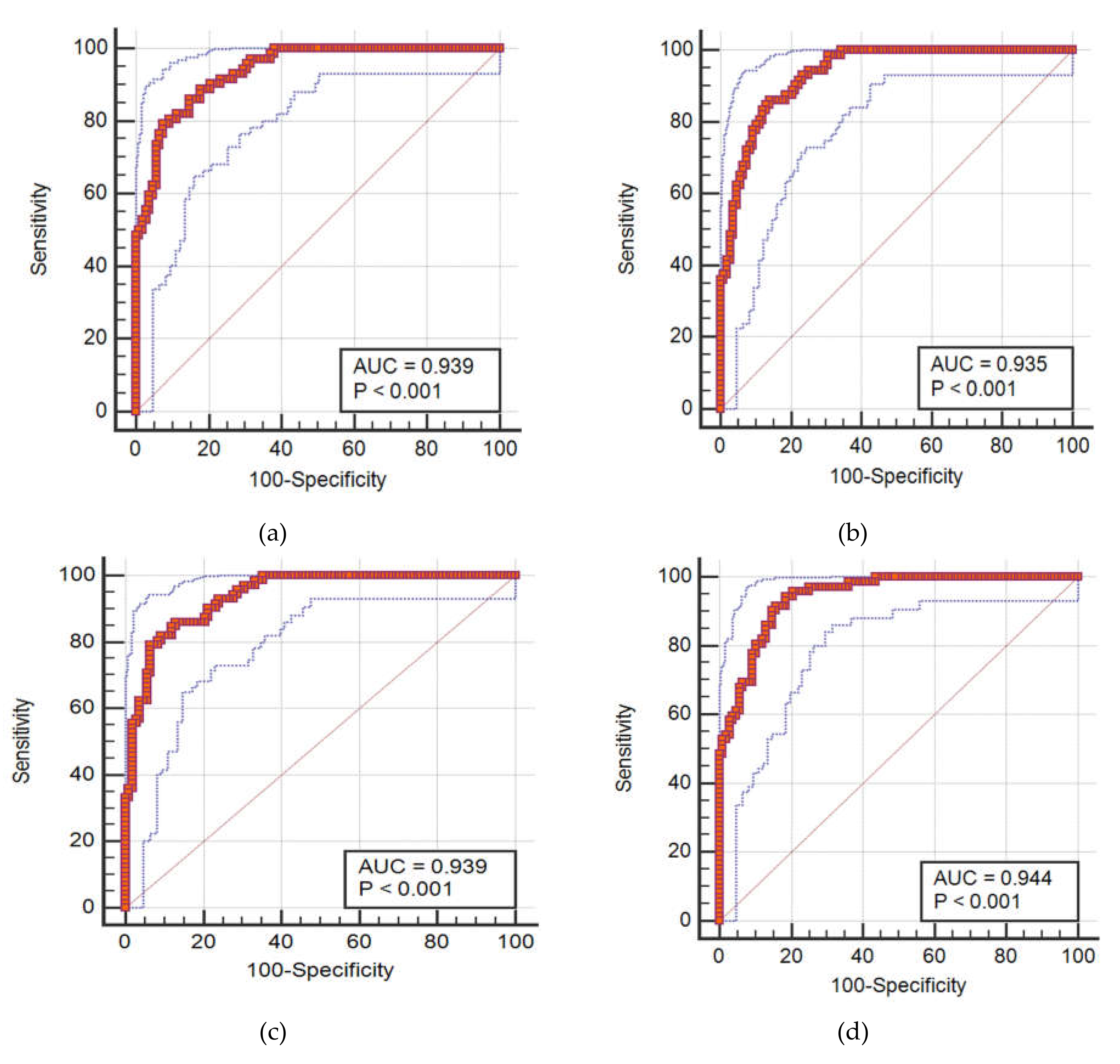
| WOA–ANN | 0.3076 | 0.2555 | 0.969 | 0.3399 | 0.2832 | 0.939 |
| LCA–ANN | 0.3122 | 0.2592 | 0.964 | 0.3426 | 0.2868 | 0.935 |
| MFO–ANN | 0.2985 | 0.2430 | 0.969 | 0.3330 | 0.2706 | 0.939 |
| ACO–ANN | 0.2745 | 0.1783 | 0.965 | 0.3133 | 0.2128 | 0.944 |
| Models | Scores | |||||||
|---|---|---|---|---|---|---|---|---|
| Training | Testing | |||||||
| RMSE | MAE | AUROC | Score | RMSE | MAE | AUROC | Score | |
| MLP | 1 | 1 | 2 | 4 | 1 | 1 | 2 | 4 |
| WOA–ANN | 3 | 3 | 5 | 11 | 3 | 3 | 4 | 10 |
| LCA–ANN | 2 | 2 | 3 | 7 | 2 | 2 | 3 | 7 |
| MFO–ANN | 4 | 4 | 5 | 13 | 4 | 4 | 4 | 12 |
| ACO–ANN | 5 | 5 | 4 | 14 | 5 | 5 | 5 | 15 |
© 2019 by the authors. Licensee MDPI, Basel, Switzerland. This article is an open access article distributed under the terms and conditions of the Creative Commons Attribution (CC BY) license (http://creativecommons.org/licenses/by/4.0/).
Share and Cite
Moayedi, H.; Bui, D.T.; Thi Ngo, P.T. Neural Computing Improvement Using Four Metaheuristic Optimizers in Bearing Capacity Analysis of Footings Settled on Two-Layer Soils. Appl. Sci. 2019, 9, 5264. https://0-doi-org.brum.beds.ac.uk/10.3390/app9235264
Moayedi H, Bui DT, Thi Ngo PT. Neural Computing Improvement Using Four Metaheuristic Optimizers in Bearing Capacity Analysis of Footings Settled on Two-Layer Soils. Applied Sciences. 2019; 9(23):5264. https://0-doi-org.brum.beds.ac.uk/10.3390/app9235264
Chicago/Turabian StyleMoayedi, Hossein, Dieu Tien Bui, and Phuong Thao Thi Ngo. 2019. "Neural Computing Improvement Using Four Metaheuristic Optimizers in Bearing Capacity Analysis of Footings Settled on Two-Layer Soils" Applied Sciences 9, no. 23: 5264. https://0-doi-org.brum.beds.ac.uk/10.3390/app9235264