Modeling and Analysis Framework for Investigating the Impact of Dust and Temperature on PV Systems’ Performance and Optimum Cleaning Frequency

Abstract

This paper proposes computational models to investigate the effects of dust and ambient temperature on the performance of a photovoltaic system built at the Hashemite University, Jordan. The system is connected on-grid with an azimuth angle of 0° and a tilt angle of 26°. The models have been developed employing optimized architectures of artificial neural network (ANN) and extreme learning machine (ELM) models to estimate conversion efficiency based on experimental data. The methodology of building the models is demonstrated and validated for its accuracy using different metrics. The effect of each parameter was found to be in agreement with the well-known relationship between each parameter and the predicted efficiency. It is found that the optimized ELM model predicts conversion efficiency with the best accuracy, yielding an R² of 91.4%. Moreover, a recommendation for cleaning frequency of every two weeks is proposed. Finally, different scenarios of electricity tariffs with their sensitivity analyses are illustrated.

1. Introduction

Solar energy systems, especially photovoltaic (PV) systems, have become one of the main electricity providers in the last decade, because the cost of their components and installation has dropped dramatically since the 1990s [1,2]. However, climatic, environmental and operative conditions, as well as geographical locations, play crucial roles in the energy yield of such systems. This fact has triggered the motivation for research into quantifying and modeling the output power/efficiency of PV systems as a function of such conditions. Researchers are investigating dust accumulation, soiling effects and temperature on PV performance and are trying to maximize the energy yield and minimize the power loss due to these factors. The country of Jordan is one of the Middle East and North Africa (MENA)-region countries and has some of the highest dust emission and deposition flux in the world [3]; in addition, this region controls dust distribution in other parts of the world [3,4].

Due to its importance and influence on PV performance, several review papers have been published that target the classification and categorization of the work accomplished in this field. For instance, in [5], the published work since 2010 was summarized. In their review, Mani and Pillai [6] reviewed the work done before and after 1990, and they came up with general recommendations for different temperature ranges and amounts of annual precipitation. As far as the country of Jordan is concerned, they recommended a cleaning frequency of once a week or two times a week based on the rate of dust accumulation. In their review paper [7], a summary of dust effects on PV performance and the chemistry and physics of dust particles along with restoration and preventive mitigation is presented. Meral et al. [8] concluded that cell technology, the selection of equipment, temperature and dust have a huge influence on the PV efficiency. A review that deals with the mechanisms of dust accumulation, rebound and resuspension is shown in [9]; they discussed the effects of air velocity and direction, and humidity for each mechanism. It was concluded that soiling is greatly affected by the module tilt angle while the resuspension mechanism is the most sensitive to wind velocity and has the highest dependence on the particle size. A balance between dust losses and cleaning expenses is presented in [10]. Different models were developed to predict the variable power output of PV. A detailed review of these models is presented in [11]. They reported that the regression models have an advantage as far as the metrological variables are concerned, while intelligent learning techniques can offer improved nonlinear approximation performance. In their review, Madeti et al. [12] show that harsh environmental conditions could reduce the reliability of sensors used for PV parameters measurements, increasing malfunction. Mekhilef et al. [13] stated that humidity affects the incident irradiance as well as the dust accumulation. Moreover, they concluded that increasing air velocity decreases the cell temperature and increases dust accumulation. Since PV technology is booming in the MENA region, many researchers in the region have worked on trying to investigate the effect of dust and soiling on PV performance. For example, a study in a controlled experimental setup to investigate the effect of dust on the reduction of PV efficiency was conducted in Baghdad, Iraq in [14]. It was concluded that efficiency reduced by 6.24%, 11.8% and 18.74% for dust exposures of one day, one week and one month respectively. Their results are in excellent agreement with the results obtained mathematically in [15]. In their work, Abed et al. [16] investigated the effects of Khamaseen (Haboob) dust storms coming to Jordan from the Arab Peninsula on PV performance as well as the environmental and health issues caused by such storms. They found that the major particles in such storms are aluminosilicates with a particle size of 5–20 mm. Moreover, they concluded that such storms affect the PV system performance significantly. During the period from February to May in Southern Libya, the effect of dust on PV performance was analyzed experimentally [17]. They concluded that there is a performance loss due to dust which ranges between 2% and 2.5%.

Inspecting the published work discussed in the area of investigating the effects of operating and ambient conditions on the performance of the PV system, it is concluded intuitively that the effect of ambient temperature, irradiance, cell temperature and wind speed on PV systems depends on geographical location and environmental and meteorological conditions. Researchers around the world strive for better comprehension of the impact of these parameters on PV systems. Understanding the effect of these parameters is realized by designing robust and reliable theoretical models and/or conducting experiments. For instance, correlations of solar electrical efficiency and power dependence on temperature were reviewed in [18]. Kim et al. [19] reported that the power and efficiency of PV modules drop as the ambient temperature increases. It was found in the work conducted by [19] for PV modules equipped with fins at the backside that the maximum power decreases as the ambient temperature increases. Moreover, an experimental study to investigate the effect of the dry bulb temperature on the performance of the thin-film PV module was carried out by [20], and it was concluded that the dry bulb temperature has a significant effect on the open circuit voltage and less effect on the short circuit current. Additionally, effects of the ambient temperature and wind speed on the PV module temperatures were simulated in a parametric study in the work presented by [21], it was found that the module temperature decreases with wind speed at constant ambient temperature. Finally, in the experimental work conducted in Abu-Dhabi to investigate the effects of solar irradiance, wind speed, relative humidity and ambient temperature on a thin film grid-connected PV system, presented in [22], it was concluded that both the open-circuit voltage and short-circuit current drop as the ambient temperature increases.

Based on the above-mentioned literature review, and since soiling and dust have a significant impact on the PV performance, it is crucial to design models that can predict PV performance. The complexity of these models increases as the number of parameters and factors taken into consideration increases. For example, Pulipaka et al. [23] proposed a neural network model to predict the PV power output as a function of the chemical, physical and spectral characteristics of the soil, and they concluded that the neural network hybrid performed well compared to other networks. In the work of Pulipaka et al. [24], both neural network and regression models were proposed to predict the PV power loss resulting from artificial soiling. They concluded that the regression model fits well for a specific irradiance range and some types of soil, while the neural network model succeeds in other ranges of irradiance and different types of soil. In Italy, a study was conducted by Pavan et al. [25] to investigate the effect of soil on PV power loss, and two models to predict the power loss, namely the Bayesian neural network and polynomial regression, were proposed. It was shown that the results of both models show excellent agreement, with power losses of 5.25% and 1.01% for PV systems installed on sandy and green lands, respectively. In order to investigate the effect of the particle size on the PV soiling losses, in a study conducted by Mani et al. [26], a multiple variable regression model as a function of the irradiance, tilt angle and particle size is proposed. It was shown that for a tilt angle of 18, and when particle sizes of less than 75 mm diameter are dominant, the optimal tilt angle deviates by 4° from the optimal tilt angle of the clean module. Moreover, it was shown that when particle sizes of 150–300 mm are dominant, the deviation in the optimal tilt angle is 8° from the clean module angle. Artificial soiling experiments to investigate the relationship between irradiance, tilt angle and power output with soil particle deposition were conducted by Pulipaka et al. [27]: they introduced a correction factor as a function of the particle size in the regression model, and by doing so, a much better efficiency prediction is achieved. The effects of local environmental conditions in Surabaya, Indonesia on the reduction in PV power output were investigated by [28]; their results illustrate that the dust accumulation after two weeks’ exposure in a dry season resulted in a 10.8% reduction in PV output power. Additionally, it was shown in the work presented in [29] that out of more than 17 pollutants, six had a significant effect on PV performance. A mathematical formulation for the optimum cleaning interval depending on the dust accumulation and the cost of cleaning operation in central Saudi Arabia was presented in [30]: they concluded that the highest loss rates occur in the spring season due to the dust storms. The authors emphasize that this conclusion is exclusive for this site and corrections to the model should be taken into consideration for other geographical and climatic conditions. An experimental study in Chang’an District, Xi’an, China, to investigate the impact of dust deposition on the module temperature, transmittance and output power of the PV module was carried out by [31]. They derived a linear model to predict the output power as a function of the deposition density, and they showed that as the deposition density increases, the relative transmittance and output power drop compared to clean modules. Also, an experimental study to investigate the effect of normal dust, clay and ash on PV performance is illustrated in [32]: they showed that the maximum power loss was 36.7% at 258 W/m² and was mainly because of the carbonaceous ash and clay.

To solve the problem of dust accumulation and reduction in the output power generated from the PV modules, cleaning is a key feature from an economic as well as performance standpoint [33]. Consequently, a weekly or bi-weekly cleaning cycle for PV systems installed in the MENA region is recommended [34]. Many experiments that tackle the effect of the cleaning cycle on the PV performance have been conducted in the last few decades. For instance, an experiment in the west of Saudi Arabia was conducted, where the performances of different modules were monitored, as well as two sand abrasion methods investigated, based on the transmittance and reflectance of PV modules [35]. It was concluded that significant dust deposition and lack of rainfall led to a loss in the daily average performance. Moreover, much higher losses were recorded during dust storms. Another experiment was conducted in Egypt in [36] to investigate the effect of daily cleaning for 45 consecutive days on the performance of the PV system. It was shown that a non-pressurized water system will not clean the panels properly, while pressurized water will but with a penalty of an increase in the running cost. In another experimental study in Egypt [20], it was demonstrated that dust has an important effect on the short-circuit current and less effect on the open-circuit voltage. Moreover, it was recommended to clean the panels once every four days. A comparison between nano-coated self-cleaning panels to untreated panels was executed experimentally in Algeria [37]. It was shown that nano-coated panels have better performance with a lower cleaning cost compared to conventional methods. In their work, Maghami et al. [38] classified shading due to soiling into two types: soft shading resulted from the airborne materials, and hard shading due to accumulated soil on the PV surface. It was reported that soft shading affects the current whereas hard shading affects the voltage. Thus, cleaning on a daily basis was recommended for severe accumulation, and on a weekly basis in the dry season. Results from an experiment conducted in Belgium by [39] showed that there is a constant power loss of 3–4% for a 35° tilt angle due to dust effects. In addition, it was concluded that rainfall definitely helps in cleaning large particles but has only a slight effect on smaller ones. It was shown in [40] that cleaning dust using nylon brushes will not have a significant effect on the optical parameters of the glass surface. However, the cleaning efficiency is not high compared to water cleaning using soft wipers. The derivation of a mathematical model to calculate cleaning frequency for PV panels is done in [41]; the suggested model is a function of particle accumulation density, particle deposition velocity, and particle mass concentration. It was shown that for a reduction of power output of 5%, a cleaning frequency of 20 days is recommended for desert regions.

It is worth mentioning that modeling PV efficiency as a linear function of dust accumulation and ambient temperature is valid and supported by observation and experiments published by other researchers [42,43,44,45,46]. A brief review of the energy yield losses caused by dust deposition on PV systems is reported in [42]. A number of experiments supporting the assumption of a linear approximation for efficiency reduction versus dust deposition is presented in this review. Another study focusing on the effect of tilt angle on soiled PV panels was conducted and proposed an empirical 2nd polynomial correlation of power reduction as a function of the number of unclean days and tilt angle [43]. The coefficients of linear terms are significantly larger than those of the quadratic terms. The soiling losses are found to aggregate linearly with time in two studies performed in California, USA [44,45]. A decrease in efficiency varying from 7.2% to 5.6% during 108 days of the dry period in the summer was noted [44]. In addition, it was stated that there were losses of 7.4% and 13.9% in efficiency for an average of 145 days of summer drought and more than 145 days of drought, respectively [45]. Experiments for a 3-month period in the Sahara area, Algeria, for PV modules for different dust densities were conducted in [46]. The reduction in efficiency was modeled by a polynomial expression of the 3rd order, with the coefficient of linear term being very large compared to the coefficients of the quadratic and cubic terms by one and two orders of magnitudes, respectively.

In short, and by revisiting the introduction above, it is obvious that the combined effect of dust accumulation and ambient temperature on PV systems depends on environmental and metrological conditions as well as the geographical location. It is important to investigate the effect of such parameters so that the power loss can be minimized. Additionally, many researchers have tried to find the best cleaning method and frequency. In this research, we build simple and accurate mathematical models based on the actual performance conditions to predict the behavior of a PV system and determine its optimum cleaning frequency. This work aims to add a significant contribution to the PV literature. In this work, we have experimentally collected PV system parameters during a 192-day period under real conditions. Based on the performance parameters, two models are developed to predict the system output behavior employing optimized artificial neural network (ANN) and optimized extreme learning machine (ELM) models [47]. It is worth mentioning that ANN and ELM have been widely developed and applied for different applications; for instance, ANN and ELM models are used in the fields of sustainability [48] speech recognition [49] medical [50] and load monitoring [51] environment [52] and hardware [53] respectively. The two models considered the dust accumulation and the ambient temperature as the independent variables and PV conversion efficiency as the dependent variable. A detailed comparison between the two models in terms of their features and accuracy is presented. Moreover, an estimation of the losses due to dust accumulation along with cleaning frequency is shown. The authors believe that this work will serve as a powerful tool for investors and stakeholders in the MENA region that predicts system performance based on the ambient temperature and dust accumulation. Moreover, this paper will provide the optimum cleaning frequency for PV systems.

The aforementioned introduction discussed the effect of dust accumulation and the ambient temperature on PV system performance, along with cleaning techniques and frequencies for such systems. The remainder of the paper is divided as follows: Section 2 describes the experimental set-up and data collection for an experimental study in Zarqa, Jordan. Section 3 presents the models developed in this paper. This is followed by the results and a discussion of these models in Section 4. Section 5 will address the cleaning of the PV system. Finally, a summary of major findings and conclusions about the importance of this research is reported in Section 6.

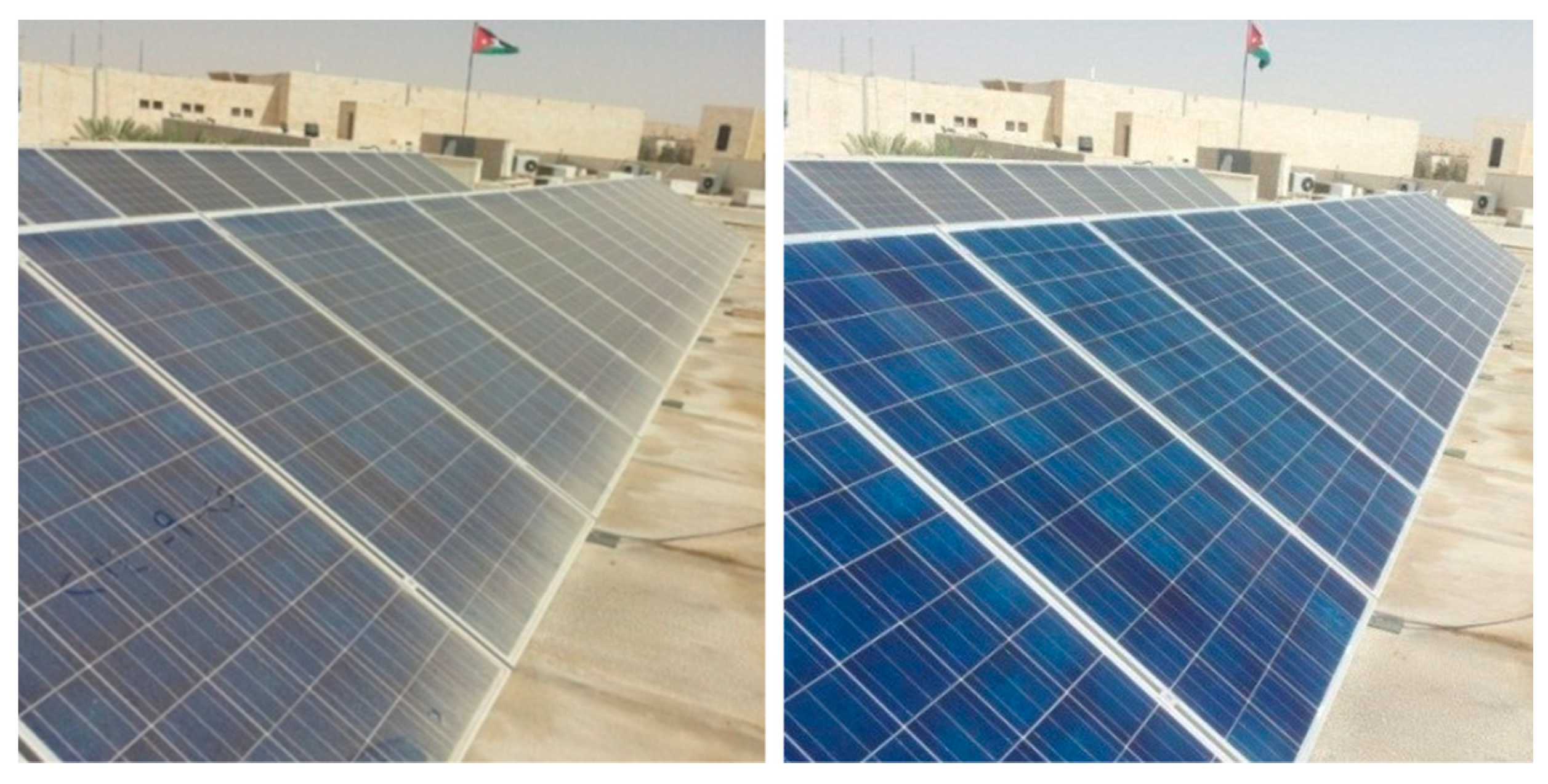
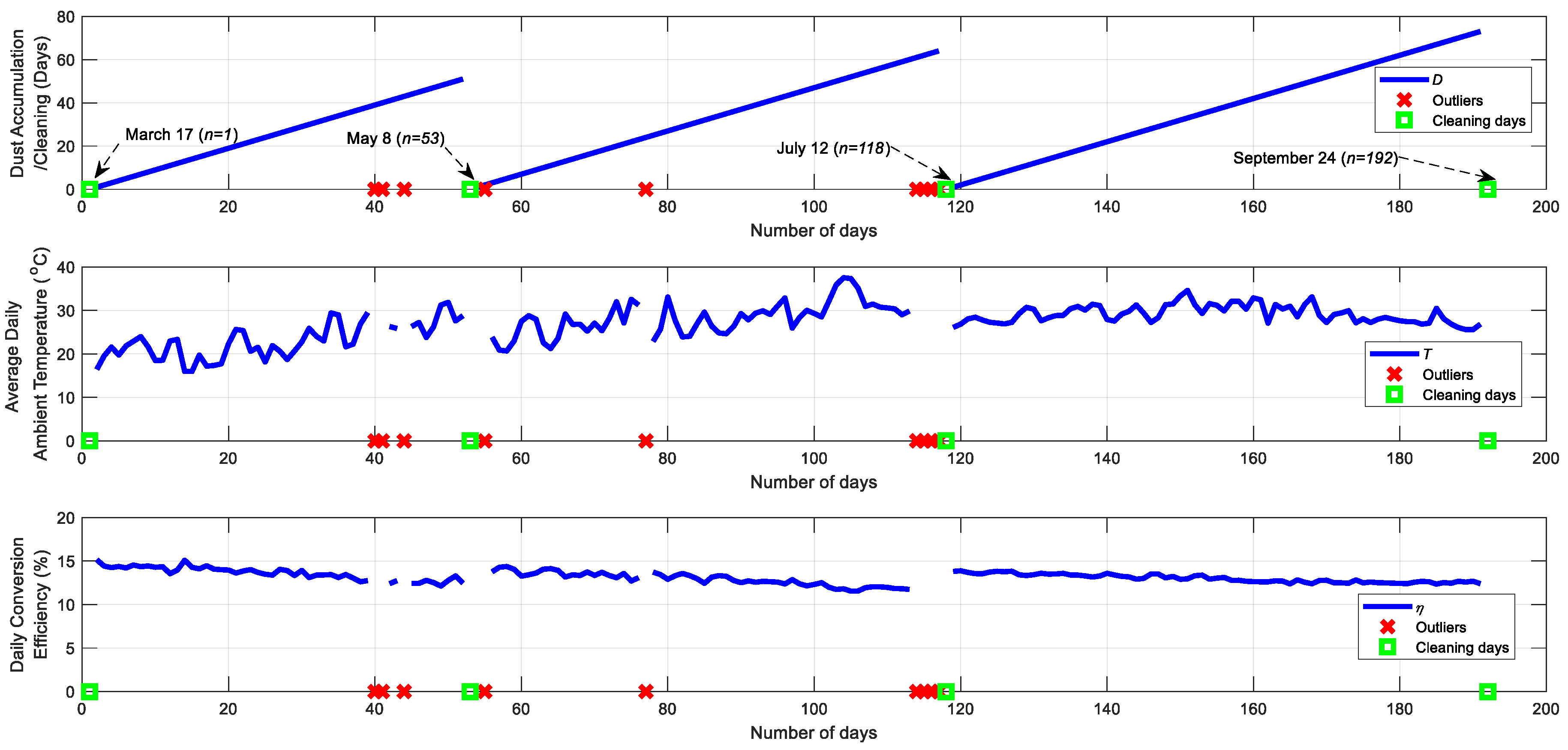
2. Experimental Setup and Data Collection

The rooftop system is installed at the Hashemite University (HU) in Zarqa, Jordan, at latitude of 32.1022° N, longitude of 36.1850° E and an altitude of 575 m. The system is grid-connected, consisting of 28 modules of a nominal power of 285 Wp (STP285–24/Vd) [54] wired in two strings with a nominal system power of 7.98 kWp, as pictured in Figure 1 [55]. The tilt angle of the system is 26°, which is equivalent to 0° azimuth angle. The two strings are connected to a 3-phase 8 kW invertor (PVI-8.0-TL-OUTD, ABB) [55]. The system is integrated to a data acquisition system to collect several inputs and outputs at different time intervals, which was set to one minute. The data was collected from 17 March 2014 to 24 September 2014. The system was cleaned by rainfall on 17 March and 8 May, whereas manual cleaning was performed on 12 July and 24 September. However, it was found that 9 data points out of 192 were outliers, with excessive efficiency values traced to sensor malfunctions. In addition, the four cleaning days were excluded from further analysis because cleaning was done during the day, which implies that the data collected during these days is not reliable (part of the day has dust accumulated on the PV modules, and the other part is clean). Thus, 179 data points were used for further analysis. The system outputs and climatic data are collected every minute, displayed in real-time, and stored and accessed by authorized persons. However, the data was manipulated on an hourly average basis, as shown later in the analysis section.

In this work, we consider that the rain and manual cleaning result in the same cleanness for the PV system. This is due to the fact that the manual cleaning was done with water and special brushes, and the rainfall cleaning was done in heavy rain with the same special brushes. In both cases, the visual inspection after cleaning revealed that the cleanness was the same. This would justify the appropriateness of this assumption. In other words, although the details of cleaning are not mentioned in this manuscript, the level of cleanness was controlled by applying brushing to the PV panels right after heavy rain and with manual water cleaning.

The performance of the 7.98 kWp PV system is evaluated based on IEC 61724 (1998) [56]. The system conversion efficiency, $\eta$, is defined as the ratio of the net AC output energy, $E_{out}$, to the input solar energy. It is important to mention here that all the energy losses due to cables, invertors, orientation, etc. are taken into consideration in the definition of the system conversion efficiency.

The system conversion efficiency is mathematically defined as

$$\eta = E_{out}/\left(H\times A\right),$$

(1)

where $A$ is the total area of the modules, which is 49.061 m², and $H$ is the total daily global incident irradiance.

For clarification purposes, Figure 2 shows the dust accumulation (represented in terms of exposure days) (Figure 2 (top)), the calculated average daily ambient temperature (Figure 2 (middle)), and the calculated system daily conversion efficiency based on the daily AC electric output and the total daily global incident irradiance (Figure 2 (bottom)), for the whole study period, with $n=179$ data points. Looking at Figure 2, one can see the sudden rises in the system conversion efficiency, which are due to the cleaning effect of the PV modules; i.e., at these times, the PV system had been cleaned.

For the prediction purposes of the system’s daily conversion efficiency using the proposed models, the overall collected data are divided into two sets of data:

• Training and validation sets of data: 80% of the overall data (i.e., 143 data points) is selected randomly for the purpose of building the prediction models. Among these, 70% and 30% of data points are further selected randomly, internally by the ANN and ELM models, for the purpose of training and optimizing the prediction models, respectively;
• Test set of data: the remaining 20% (i.e., 36 data points) is used to evaluate the prediction performance of the proposed prediction models with respect to those previously proposed and developed in Hammad et al. [54]. This set of data was never introduced to the prediction models during the training phase.

It is worth mentioning that the division of the data is performed similarly to that in Hammad et al. [54] for fair comparison.

In other words, the data is split into 80% for developing the prediction models and 20% for further testing and inspection. The 80% split is called the training set and the 20% split is called the blind set (where the model does not use this part of the data during the development process). The split of the training set into training, validation and testing is a well-established method in neural network development and is a built-in feature in Matlab. The ratios for each part (70%–15%–15%) are the defaults to train and optimize the network architectures.

3. Methodology

PV system output power, conversion efficiency and energy yield decrease as dust accumulation increases. This is mainly due to the fact that, as dust accumulation increases, transmittance through the PV glass covers decreases and the reflectance of incident irradiance increases. Moreover, as the ambient temperature increases, the module temperature increases, causing the generated power to decrease [8,57,58,59].

This work aims at developing optimized versions of single hidden layer artificial neural network (ANN) [60,61,62] and extreme learning machine (ELM) models [47] to predict and estimate the daily system conversion efficiency as a function of dust accumulation and average daily ambient temperature. The proposed models are compared to the models proposed and developed with the same dataset for the same purpose, namely the multivariate linear regression (MLR) model and two hidden layer ANN models [54].

For completeness, Section 3.1, Section 3.2 and Section 3.3 are devoted to providing brief descriptions of the MLR, ANN and ELM models, respectively, whereas Section 3.4 presents the standard performance metrics of the literature considered for evaluating the performance of the prediction models.

3.1. Multivariate Linear Regression (MLR) Model

MLR aims to build an appropriate mathematical equation that relates a set of independent variables (i.e., predictors or causal variables) to the dependent variable (i.e., response variable). Specifically, the dust effect (represented in terms of exposure days ($D$)) and the average daily ambient temperature ($T$) are considered as independent variables, whereas the daily system conversion efficiency ($\eta$) is considered as the dependent variable. Thus, the mathematical equation provided by the MLR can be written as follows [54]:

$${\eta }_i=a_o+a_1{D}_i+a_2{T}_i+{\epsilon }_i,$$

(2)

where ${\eta }_i$ is the $i$-th daily system conversion efficiency, $D_i$ is the $i$-th exposure day, $T_i$ is the $i$-th average daily ambient temperature, $a_o$ is the regression model intercept, $a_1$ and $a_2$ are the regression coefficients, and ${\epsilon }_i$ is the $i$-th error of the daily system conversion efficiency (i.e., the difference between the true and predicted daily system conversion efficiencies of the $i$-th day), $i=1,\dots ,n$.

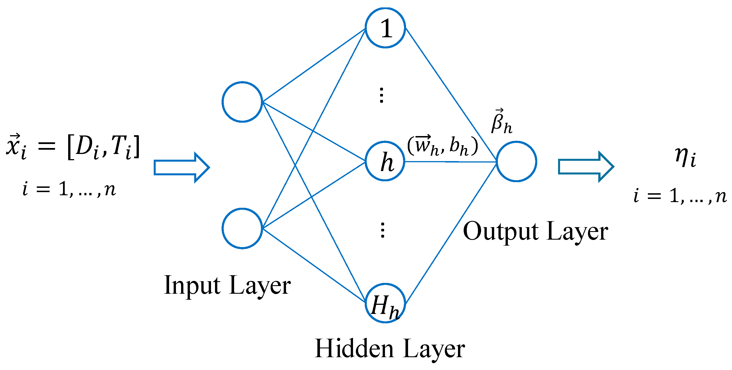
3.2. Artificial Neural Network (ANN) Model

An artificial neural network (ANN) model is defined as interconnected mathematical systems of neurons that interchange communication among themselves [60,61,62]. The ANN is a computational model employed to capture the hidden relationship between a set of numerical input data to a set of numerical target data. Basically, the ANN model (depicted in Figure 3) comprises three layers, namely input, hidden, and output layers, with sufficient number of neurons, $H_i$, $H_h$ and $H_o$, respectively. In practice,

• the input layer receives the $i$-th data point (${\overrightarrow{x}}_i$) that comprises the dust accumulation in terms of exposure days ($D_i$) and the average daily ambient temperature values ($T_i$) (i.e., $H_i=2$), ${\overrightarrow{x}}_i=\left[D_i,T_i\right], i=1,\dots ,n$;
• the hidden layer manipulates them through the so-called hidden neuron activation function, $G()$, to define the output of each $h$-th hidden neuron, $h=1,\dots ,H_h$, based on the received inputs;
• the output layer receives the processed information and provides the $i$-th daily system conversion efficiency (i.e., $H_o=1$) by the following equation [62]:

  $${\eta }_i={\displaystyle \sum }_{h=1}^{H_h}{\overrightarrow{\beta }}_{h}G\left({\overrightarrow{w}}_h{\overrightarrow{x}}_i+b_h\right),$$

  (3)

  where ${\overrightarrow{w}}_h$ (the input weights vector that connects the inputs to each $h$-th hidden neuron), $b_h$ (the input bias of each $h$-th hidden neuron), and ${\overrightarrow{\beta }}_h$ (the output weights vector that connects the outcomes of each $h$-th hidden neuron to the output neuron, $h=1,\dots ,H_h$) are the internal parameters of the ANN model, and $G()$ is the hidden neuron activation function.

During the training phase, the internal parameters of the ANN model are usually defined randomly, then updated iteratively by resorting to the error back-propagation (BP) algorithm. Thus, setting the internal parameters of the ANN model requires a large computational effort to ultimately define the optimal internal parameters that lead to the accurate daily system conversion efficiency predictions [62,63].

In this work, the ANN model is an optimized version of that developed in [54] for the same purpose. The ANN proposed in [54] is a two hidden layer system composed of 10 and 4 hidden neurons. However, in this work, to further enhance the daily system conversion efficiency predictions, the ANN model is here optimized in terms of the following variables: (i) the number of hidden neurons, $H_h$, and (ii) the neuron activation function. To this end, possible candidates for the number of hidden neurons, $H_h$, and the hidden neuron activation functions are considered for identifying the optimum architecture of the ANN model by evaluating the prediction performance of the ANN architecture candidates in terms of the standard performance metrics in the literature (Section 3.4), as we shall see in Section 4.

3.3. Extreme Learning Machine (ELM)

ELM is a new learning algorithm for single and multi-hidden layer feedforward neural networks, originally developed by [47]. Similar to ANN architecture, ELM comprises three layers: input, hidden and output layers, with a sufficient number of neurons, $H_i$, $H_h$, and $H_o$, respectively (similar to the ANN architecture depicted in Figure 3). The input layer receives the dust accumulation in terms of days and the average daily ambient temperature values (i.e., $H_i=2$); then, the hidden layer manipulates them through the hidden neuron activation function, $G()$, and sends the processed information to the output layer to provide the daily system conversion efficiency (i.e., $H_o=1$).

Similar to the ANN model operation, the input weights (${\overrightarrow{w}}_h$) and biases ($b_h$) of the hidden neurons are initially defined randomly, but the output weights (${\overrightarrow{\beta }}_h$) are calculated analytically without resorting to the error BP algorithm. Thus, compared to the ANN model, ELM requires less computational effort during the training phase [47,63].

To enhance the predictions accuracy, the ELM architecture is here optimized in terms of the following variables: (i) the number of hidden neurons, $H_h$, and (ii) the hidden neuron activation function, $G()$. To this end, possible candidates for the number of hidden neurons, $H_h$, and the hidden neuron activation functions are considered for identifying the optimum architecture of the ELM model by evaluating the prediction performance of the ELM architecture candidates in terms of the standard performance metrics in the literature (Section 3.4), as we shall see in Section 4.

3.4. Performance Metrics

The effectiveness of the proposed models (the optimized versions of ANN and ELM models) in predicting the PV daily system conversion efficiency is evaluated by resorting to the following standard performance metrics in the literature for both sets of data, the training and validation datasets (i.e., 143 days) and the test dataset (i.e., 36 days) [54]:

• The coefficient of determination ($R^2$) (Equation (4)) and adjusted coefficient of determination ($R_{adjusted}^2$) (Equation (5)), which describe the variability in the dependent (output) variable provided by the prediction models caused by the two independent (input) variables only. Specifically, 100% values of these metrics entail that the variability in the output variable can be fully explained by the two considered input variables (i.e., the dust accumulation and the ambient temperature), whereas values less than 100% entail that there are other independent variables that can affect the output variable but have not been taken into account during the development of the prediction models:

  $$R^2=\left[1-\frac{S{S}_{res}}{S{S}_{tot}}\right]\times 100\%=\left[1-\frac{{{\displaystyle \sum }}_{i=1}^n{\left({\eta }_i-{\widehat{\eta }}_i\right)}^2}{{{\displaystyle \sum }}_{i=1}^n{\left({\eta }_i-\overline{\eta }\right)}^2}\right]\times 100\%,$$

  (4)

  $$R_{adjusted}^2=\left[1-\left(\frac{S{S}_{res}}{S{S}_{tot}}\right)\left(\frac{n-1}{n-2}\right)\right]\times 100\%,$$

  (5)

  where ${\eta }_i$ and ${\widehat{\eta }}_i$ are the $i$-th true and predicted daily system conversion efficiency obtained by the prediction models, and $i=1,\dots ,n$ and $n$ is the overall data size (i.e., $n=179$);
• Accuracy ($Accuracy$) (Equation (6)) describes the match between the true and the predicted daily system conversion efficiency obtained by the prediction models. Indeed, higher accuracy values entail that the predictions match the actual conversion efficiency and, thus, the prediction model is effectively capable of capturing the hidden mathematical relationship between the independent and dependent variables, and vice versa:

  $$Accuracy=\frac{{{\displaystyle \sum }}_{i=1}^n\left(1-\frac{{\eta }_i-{\widehat{\eta }}_i}{{\eta }_i}\right)}{n}\times 100\%,$$

  (6)
• Mean square error ($MSE$) (Equation (7)) describes the mismatch between the true and the predicted daily system conversion efficiency obtained by the prediction models (i.e., opposite to the $Accuracy$ metric). Apparently, small $MSE$ values are desired:

  $$MSE=\frac{{{\displaystyle \sum }}_{i=1}^n{\left({\eta }_i-{\widehat{\eta }}_i\right)}^2}{n}.$$

  (7)

4. Results and Discussion

In this section, the development of the two benchmarked prediction models, namely the MLR and the two-hidden layer ANN proposed and developed in [54] and the two proposed models, the optimized ANN and ELM, are presented. In addition, their application results are compared and discussed based on the standard performance metrics in Section 3.4.

4.1. The MLR Model

The objective of the MLR is to capture the mathematical relationship between the two independent variables (the dust accumulation and the average ambient temperature values) and the dependent variable (the daily system conversion efficiency). To this end, the multivariate regression analysis software package, Minitab (Minitab, Ltd., Coventry, UK), is employed by Hammad et al. [54] to estimate the regression model intercept and coefficients ($b’s$) associated with each variable as reported in Equation (2). Thus, the best mathematical equation that can represent the collected data ($n=143$) accurately is found to be

$${\widehat{\eta }}_i=16.0513-0.024133i-0.078743T_i,$$

(8)

where ${\widehat{\eta }}_i$ is the $i$-th predicted daily efficiency, $D_i$ is the $i$-th exposure day, and $T_i$ is the $i$-th average daily ambient temperature.

It is worth mentioning that the significance of the obtained MLR model has been evaluated and verified by resorting to the analysis of variance (ANOVA) based on the least-squares method. In addition, the adequacy and performance of the model are verified through the following [54]:

• Assumption validation: the validity and significance of the model have been examined based on some assumptions, such as residuals being normally distributed and having constant variance;
• Multicollinearity: this indicates the near-linear dependencies among the regression variables, which can lead to misleading results. To examine whether the multicollinearity does not exist in the obtained model, large variation inflation factors (VIFs) have been calculated;
• Independency of variables: to examine the correlation between the systems’ conversion efficiency and the two predictors (the dust exposure days and the average daily ambient temperature), the correlation matrix has been calculated;
• Goodness-of-fit: to verify whether the model reasonably represent the behavior of the data, the $R^2$ and its adjusted value have been computed;
• Analysis of model coefficient signs: due to the fact that the dust accumulation and the increase in the ambient average temperature will lead to a decrease in the performance of the PV system, the signs of the models’ coefficients have been verified to be negative;
• Best subsets regression: this identifies whether the obtained model can predict the conversion efficiency accurately by including all of the necessary independent variables. To this end, the $R^2$ metric has been calculated and found to achieve the highest value among the whole subset model candidates.

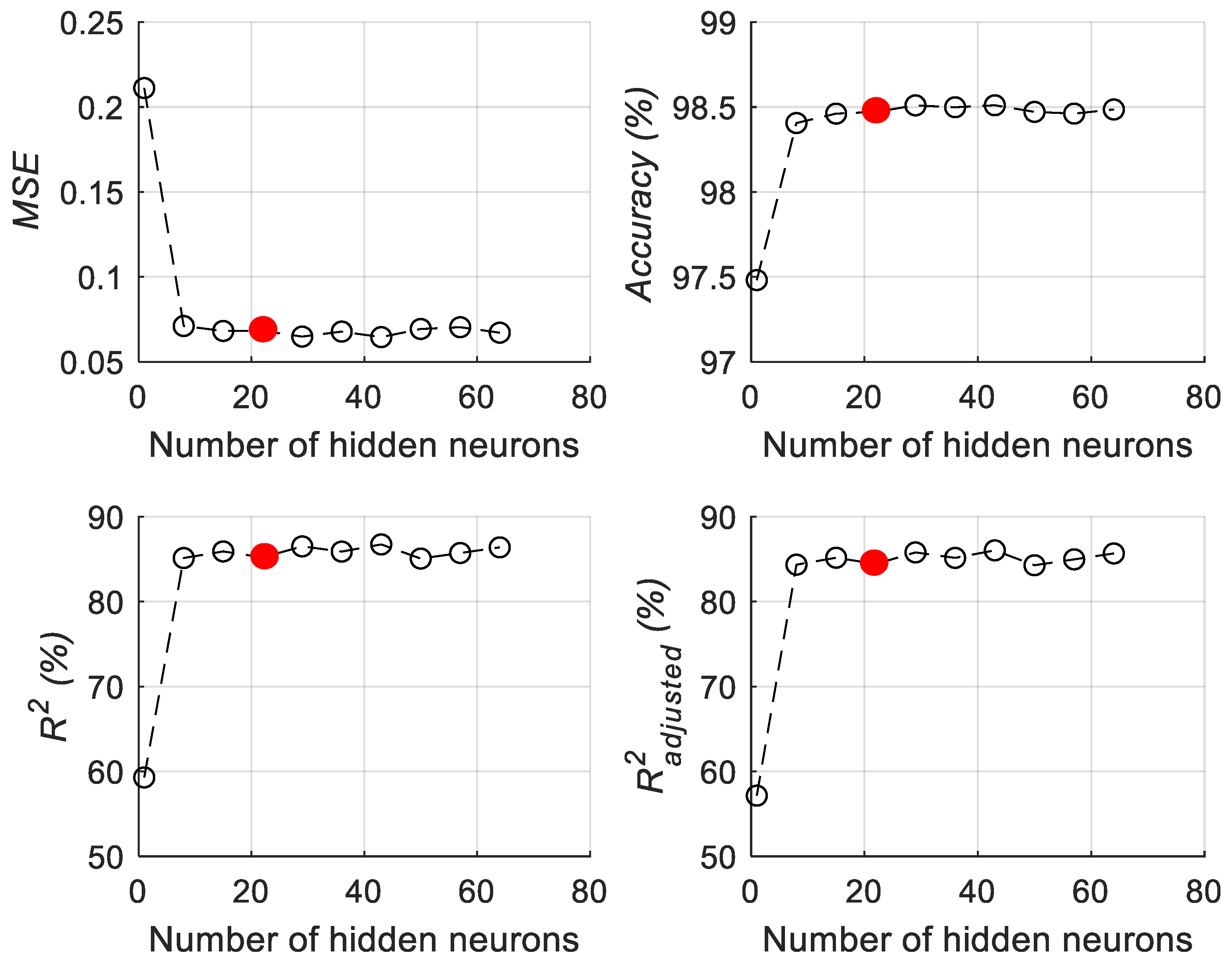
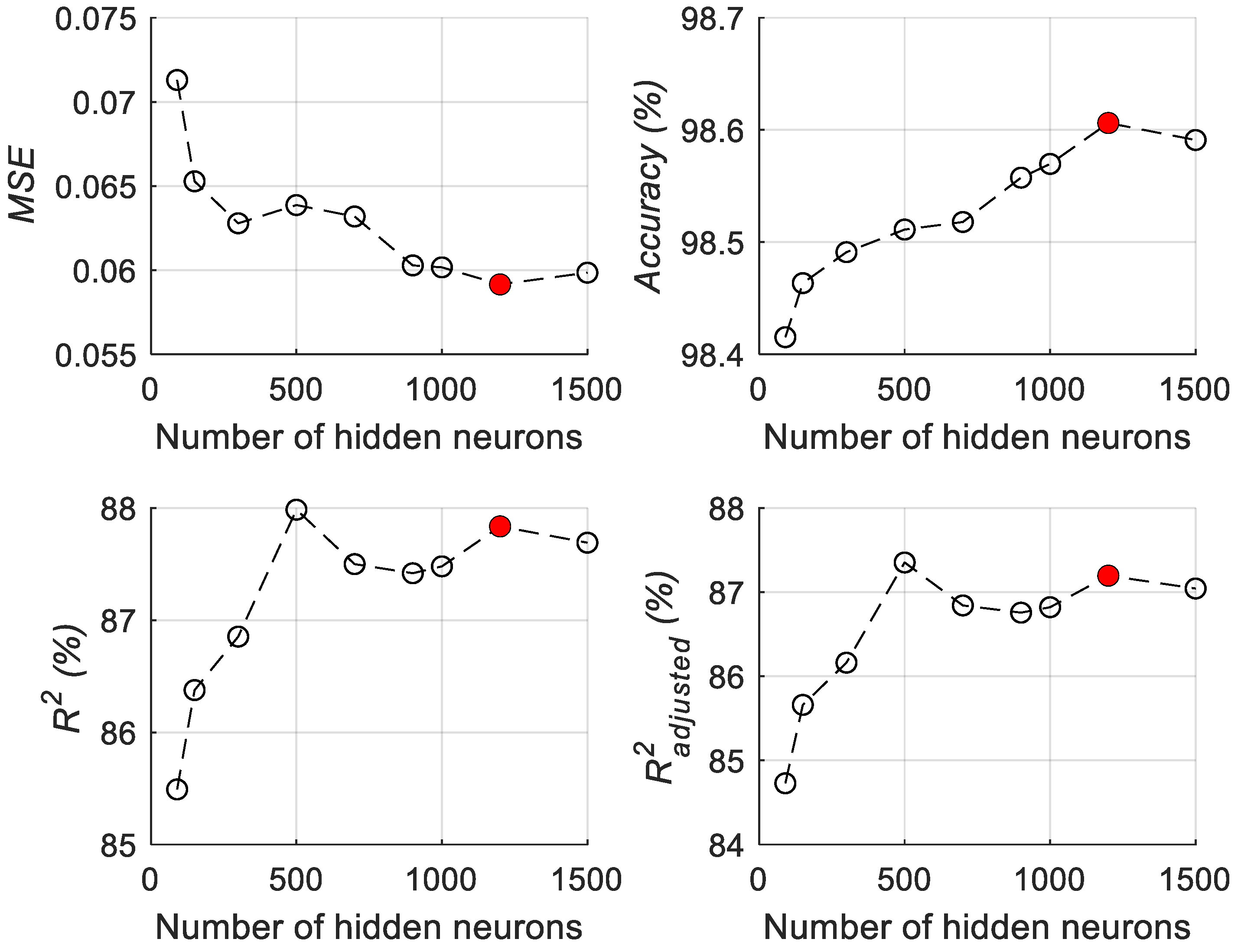
4.2. The Optimum Architecture of the ANN Model

The ANN is built in the Matlab environment using data points $n=143$, used to develop the MLR model, with the following characteristics: (i) the scaled conjugate gradient back-propagation algorithm, (ii) a root mean square error ($RMSE$) of 10^–5 to constrain the ANN training, and (iii) a maximum of 100 training epochs.

The ANN model proposed and developed in this work is an optimum version of that developed in [54] for the same purpose. The architecture of the ANN model is here optimized in terms of (i) the number of hidden neurons, $H_h$, and (ii) the hidden neuron activation function, $G()$. To this end, we follow an exhaustive searching procedure by considering possible values that span the interval [1:70] for the number of hidden neurons and 12 activation functions for the hidden neuron activation function. The 12 activation functions considered in this work are the built-in functions in the Matlab environment, such as “satlin”, “poslin”, “radbas” (interested readers can refer to [60,61,62] for more details on the ANN’s hidden neuron activation functions).

The performance of each ANN candidate architecture is evaluated by computing the standard performance metrics (Section 3.4) on the obtained predictions of the validation set of data. Specifically, 100 cross-validations procedure are carried out to robustly quantify the performance metrics: the training and validation sets of data are sampled randomly from the $n=143$ data points with fractions of 70% and 30%, respectively. The ANN model is trained and its internal parameters are optimally defined. Then, the cross-validation procedure is repeated 100 times leading to 100 values of each performance metric. The ultimate value of each metric is then computed by averaging the 100 available values on the validation set of data.

The best ANN candidate architecture is found at $H_h=22$ hidden neurons using the “poslin” neuron activation function. For clarification purposes, Figure 4 shows the influence of the hidden neurons on the four performance metrics when the “poslin” activation function is used. One can notice that the prediction performance of the ANN model increases as long as the number of hidden neurons increases; e.g., $MSE$ values decrease along with the number of hidden neurons. However, for large numbers of hidden neurons, i.e., $H_h\ge 22$, it seems that the ANN performance starts to saturate and, thus, increasing the number of hidden neurons might not be necessary to avoid the computational efforts of the ANN operation. In this regard, the optimum ANN architecture is defined by a hidden layer composed by 22 neurons using a “poslin” activation function for which the average performance metrics values on the validation set of data are $MSE=6.82\%$, $Accuracy=98.47\%$, $R^2=85.21\%$, and $R_{adjusted}^2=84.43\%$.

4.3. The Optimum Architecture of the ELM Model

Similar to the optimization procedure of the ANN model, the architecture of the ELM model is here optimized in terms of (i) the number of hidden neurons, $H_h$, and (ii) the hidden neuron activation function, $G()$. We follow an exhaustive searching procedure by considering possible values of 90, 150, 300, 500, 700, 900, 1000, 1200, and 1500 for the number of hidden neurons, and five activation functions for the hidden neuron activation function. The five activation functions considered in this work are “Triangular Basis”, “Sine”, “Sigmoid”, “Hard Limit”, and “Radial Basis” functions (interested readers can refer to [47] for more details on the ELM hidden neuron activation functions).

The performance of each ANN candidate architecture is evaluated by computing the standard performance metrics (Section 3.4) on the obtained predictions of the validation set of data by using 100 cross-validations procedure.

The best ELM candidate architecture is found at $H_h=700$ hidden neurons using the “Triangular Basis” neuron activation function. For clarification purposes, Figure 5 shows the influence of the hidden neurons on the four performance metrics when the “Triangular Basis” activation function is used. One can notice that the prediction performance of the ELM model increases as long as the number of hidden neurons increases; e.g., $MSE$ values decrease with the number of hidden neurons. However, for large numbers of hidden neurons, i.e., $H_h\ge 700$, it seems that the ELM performance starts to saturate and, thus, increasing the number of hidden neurons might not be necessary to avoid the computational effort of the ELM operation. In this regard, the optimum ELM architecture is defined by a hidden layer composed of 700 neurons using a “Triangular Basis” activation function, for which the average performance metrics values on the validation set of data are $MSE=5.92\%$, $Accuracy=98.61\%$, $R^2=87.84\%$, and $R_{adjusted}^2=87.2\%$.

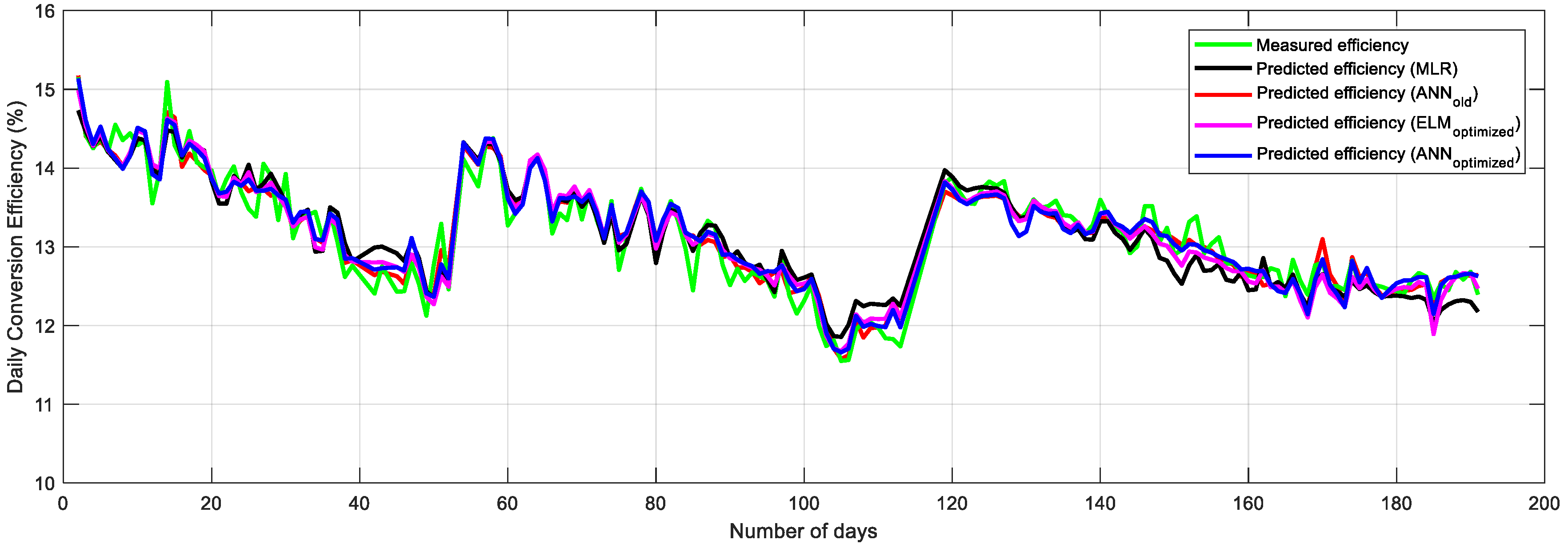
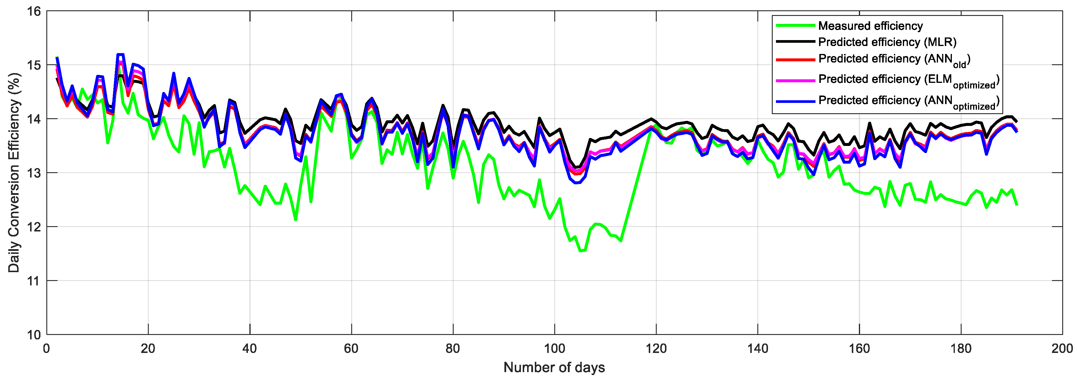
4.4. Application Results

Once the ANN and ELM models’ architectures have been defined, they are applied to the test set of data and their performances are evaluated by computing the four performance metrics on the $n=36$ data points, using the 100 cross-validations procedure. The obtained results are compared to those obtained by the two benchmarked models: the MLR and the two hidden layer ANN developed in [54].

Table 1. Comparison results of the proposed prediction models to those proposed and developed in [43]. MLR: multivariate linear regression model.

	Training and Validation Data (143 Data Points)				Test Data (36 Data Points)
	${\mathit{R}}^2$ $\left(\mathit{\%}\right)$	${\mathit{R}}_{\mathit{a}\mathit{d}\mathit{j}\mathit{u}\mathit{s}\mathit{t}\mathit{e}\mathit{d}}^2$ $\left(\mathit{\%}\right)$	$\mathit{A}\mathit{c}\mathit{c}\mathit{u}\mathit{r}\mathit{a}\mathit{c}\mathit{y}$ $\left(\mathit{\%}\right)$	$\mathit{M}\mathit{S}\mathit{E}$	${\mathit{R}}^2$ $\left(\mathit{\%}\right)$	${\mathit{R}}_{\mathit{a}\mathit{d}\mathit{j}\mathit{u}\mathit{s}\mathit{t}\mathit{e}\mathit{d}}^2$ $\left(\mathit{\%}\right)$	$\mathit{A}\mathit{c}\mathit{c}\mathit{u}\mathit{r}\mathit{a}\mathit{c}\mathit{y}$ $\left(\mathit{\%}\right)$	$\mathit{M}\mathit{S}\mathit{E}$
MLR	87.7	87.5	98.4	0.066	86.8	86.4	98.7	0.048
Two hidden layer ANN	90	89.9	98.6	0.057	89.2	88.9	98.8	0.042
Optimized ANN	90.69	90.63	98.71	0.0502	90.55	90.27	98.87	0.0331
Optimized ELM	91.42	91.35	98.74	0.0462	92.16	91.93	98.99	0.0274

reports the average performance metrics values obtained by the application of the models on the training and validation sets of data ($n=143$ data points) and the unseen test set of data ($n=36$ data points).

For clarification purposes, Figure 6 shows the measured and predicted values of the PV daily system conversion efficiency obtained by the optimized ANN and ELM models for the whole study period ($n=179$ data points) with respect to those previously obtained by the MLR and the two hidden layer ANN in [54].

The following can be observed;

• The predicted values using all models are reasonably close to the measured values for the whole study period;
• In particular, the MLR model seems to provide less accurate predictions despite its easiness and flexibility compared to the other prediction models. In fact, all performance metrics values obtained by the MLR model are worse than for the other models. This can be justified by the fact that the behavior of the PV daily system conversion efficiency as a function of dust accumulation and ambient temperature is not strictly linear; thus, it cannot be accurately captured by the inherently linear MLR model, unlike the other nonlinear models (i.e., ANN and ELM);
• The effectiveness of having an optimum version of the ANN model is apparent in the four performance metrics compared to the two hidden layer ANN model proposed in [54];
• Furthermore, the effectiveness of the ELM model with respect to the other models is proved by all performance metrics. For instance, the optimum ELM model provides an enhancement in the conversion efficiency predictions compared to the MLR model with around 6.18%, 6.4%, 0.3%, and 42.92% for the $R^2$, $R_{adjusted}^2$, $Accuracy$, and $MSE$ performance metrics.

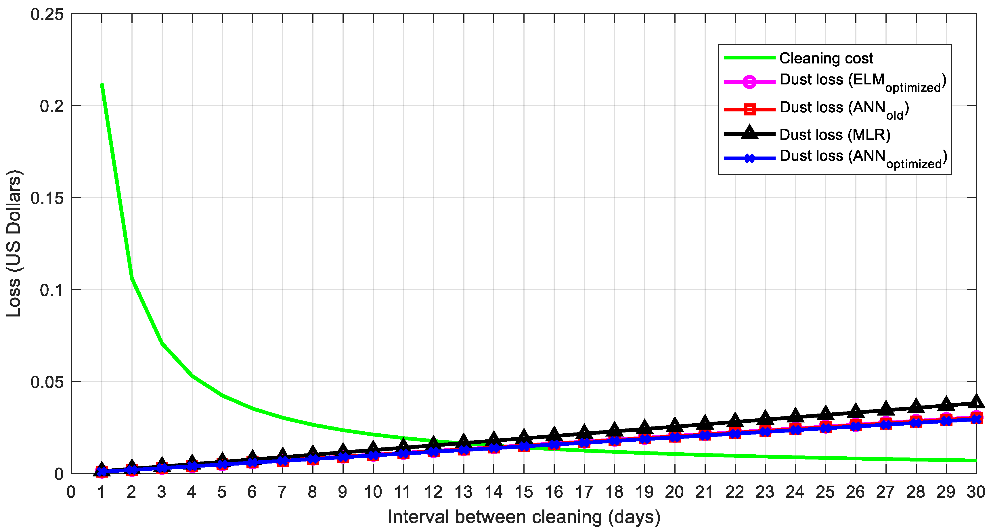
5. Cleaning of the PV System

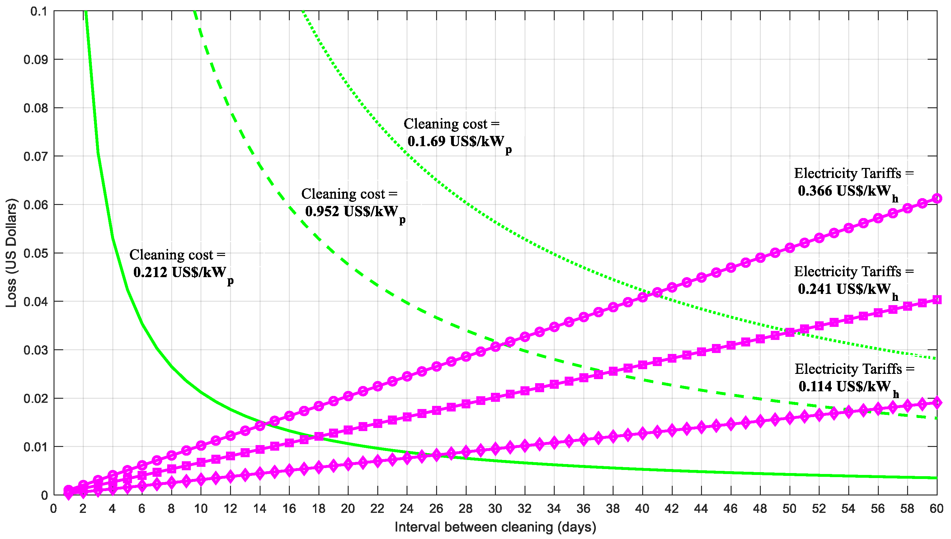
5.1. Losses and Dust Effects

Once the prediction models are developed, one can utilize them in investigating the behavior of the PV system based on a single variable, while all other variables are excluded. In this regard, the objective is to investigate the effect of the dust accumulation on the behavior of the PV system conversion efficiency. To this end, the built prediction models can then be fed with the average daily ambient temperature only, while excluding the dust accumulation (the exposure days); i.e., the exposure days variable is set to zero, which indicates that there is no dust accumulation. The output of the prediction models will be the PV daily system conversion efficiency due to all factors without the effect of dust accumulation, as depicted in Figure 7. It can be seen that the daily conversion efficiency curves no longer have decreasing trends due to dust accumulation as time passes without cleaning (refer to Figure 6).

Specifically, when comparing the actual (measured) daily conversion efficiency to the predicted one while excluding the dust effect using the optimized single hidden layer ELM model, it is found that the average daily efficiency drop is 0.615%/day. In addition, based on Equation (1), the energy loss due to the dust effect over the whole study period is found to be 8.329 kWh/m² (408.652 kWh).

Considering that the electricity tariff in Jordan (universities sector) during the study period is 0.366 US$/kWh [54], then the loss for the whole PV system will be equal to 3.76 US$/m² (US$ 184.627) with an average loss due to dust accumulation of 0.836 US$/day. For completeness, the same analysis is carried out for the other prediction models, and the obtained results are reported in

Table 2. Losses and dust effect using all investigated prediction models for the whole study period ($n=179$ days).

Model	Average Efficiency Drop (%/day)	Energy Loss (kWh/m2)	Energy Loss (kWh)	Economic Loss (US$/m2)	Economic Loss (US$)	Average Economic Loss (US$/day)
MLR	0.768	10.282	504.445	3.76	184.627	1.03
Two hidden layer ANN	0.607	8.140	399.342	2.98	146.159	0.82
Optimized ANN	0.593	7.862	385.711	2.877	141.170	0.789
Optimized ELM	0.615	8.329	408.652	3.049	149.567	0.836

.

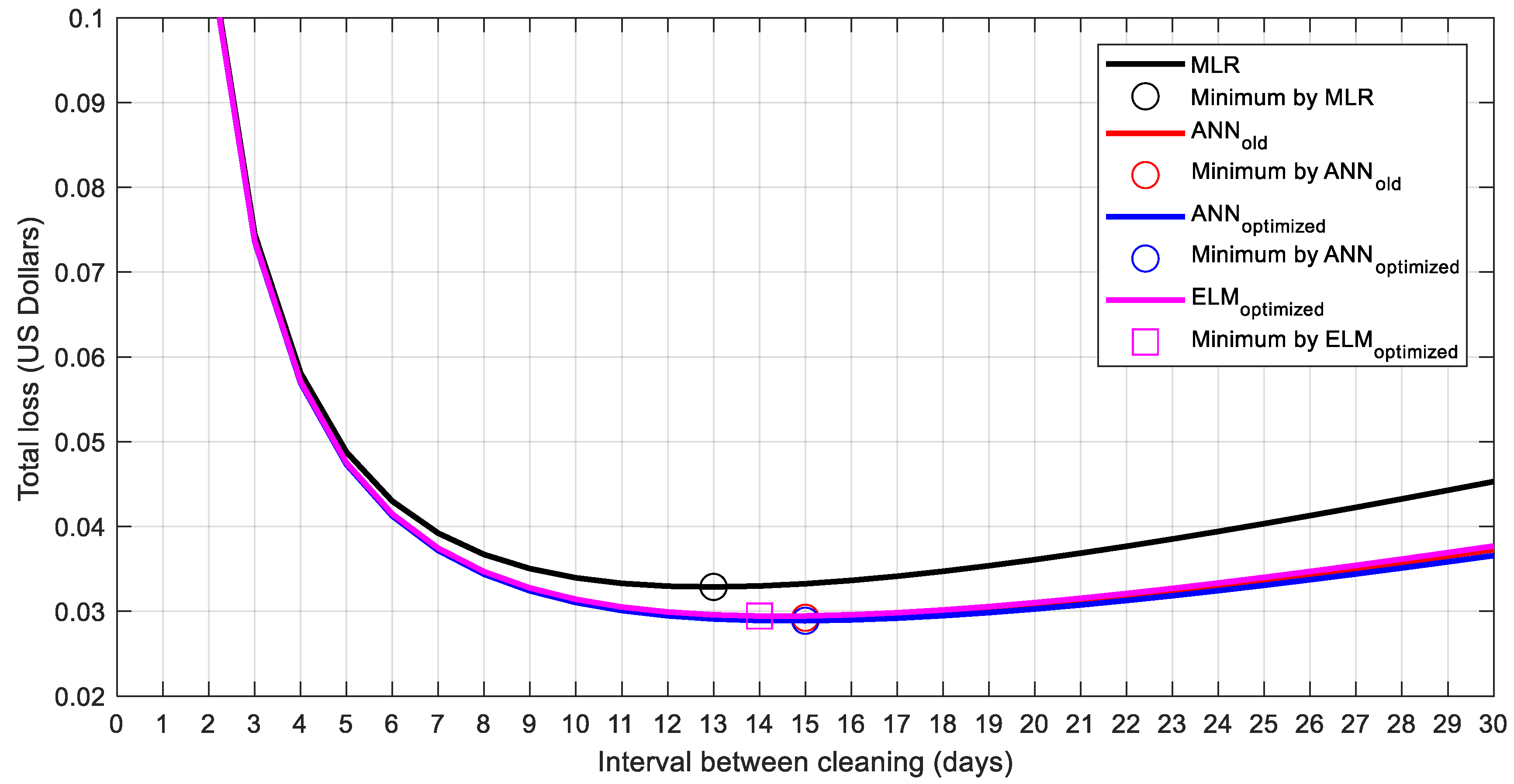
5.2. Optimal Cleaning Frequency

In this section, the optimum cleaning frequency of the PV system under study is obtained. The optimum cleaning frequency is the cleaning activity period carried out for the PV system under which the two opposing effects of cleaning are minimized, the cleaning cost of the PV system panels and the dust loss that decreases the system efficiency for a given cleaning period calculated for the study period using the prediction models.

To this end, we consider reasonable and acceptable values of cleaning costs (0.212 US$/kWp) and the electricity tariff (0.366 US$/kWh) in Jordan during the study period [54]. Firstly, the average daily expenses incurred by cleaning is computed for different cleaning periods that span the interval from 1–30 days. If the PV system is cleaned daily, then the average daily cleaning cost is 0.212 US$/kWp, whereas if the PV system is cleaned every 2 days, then the average daily cleaning cost will be 0.212/2 = 0.106 US$/kWp, leading to an inversely proportional relationship between the average daily leaning cost and period of cleaning activity. Secondly, if the PV system is cleaned daily, then the system efficiency decrease due to dust accumulation equals the average efficiency drop calculated in Table 2 using the prediction models, whereas if the PV system is cleaned every 2 days, then the system efficiency decrease equals the average efficiency drop calculated in Table 2 multiplied by 2, leading to a linear relationship between efficiency loss and cleaning periods. This decrease in the system efficiency is, then, converted into energy loss using Equation (1) and economic loss by considering the electricity tariff of 0.366 US$/kWh in Jordan.

For clarity purposes, Figure 8 shows the average daily cleaning cost (inversely proportional curve) and losses due to dust accumulation (linear curves) obtained by the four prediction models with respect to the different cleaning periods, from 1 to 30 days.

To identify the optimum cleaning frequency from Figure 8, the average daily losses due to cleaning cost (inversely proportional curve) and losses due to dust accumulation (linear curves) obtained by the four prediction models are combined as depicted in Figure 9. The optimum cleaning frequencies (i.e., the intersections of the inversely proportional linear curves of Figure 8) obtained by the MLR (13 days), two hidden layer ANN (15 days), the proposed optimized single hidden layer ANN (15 days) and ELM (14 days) models are also indicated in Figure 9, with the best optimum cleaning frequency of 14 days provided by the optimized ELM model as the best prediction model among the others (Table 1). Notice that as long as the cleaning activity occurs with a frequency less than the optimum, the cost of cleaning is the main reason for losses, whereas if the cleaning activity occurs with a frequency more than the optimum, the decrease in efficiency and energy yield is the main reason for losses. It is worth mentioning that these findings are in line with the recommendations published based on other experimental and theoretical observations for the MENA region [6,64].

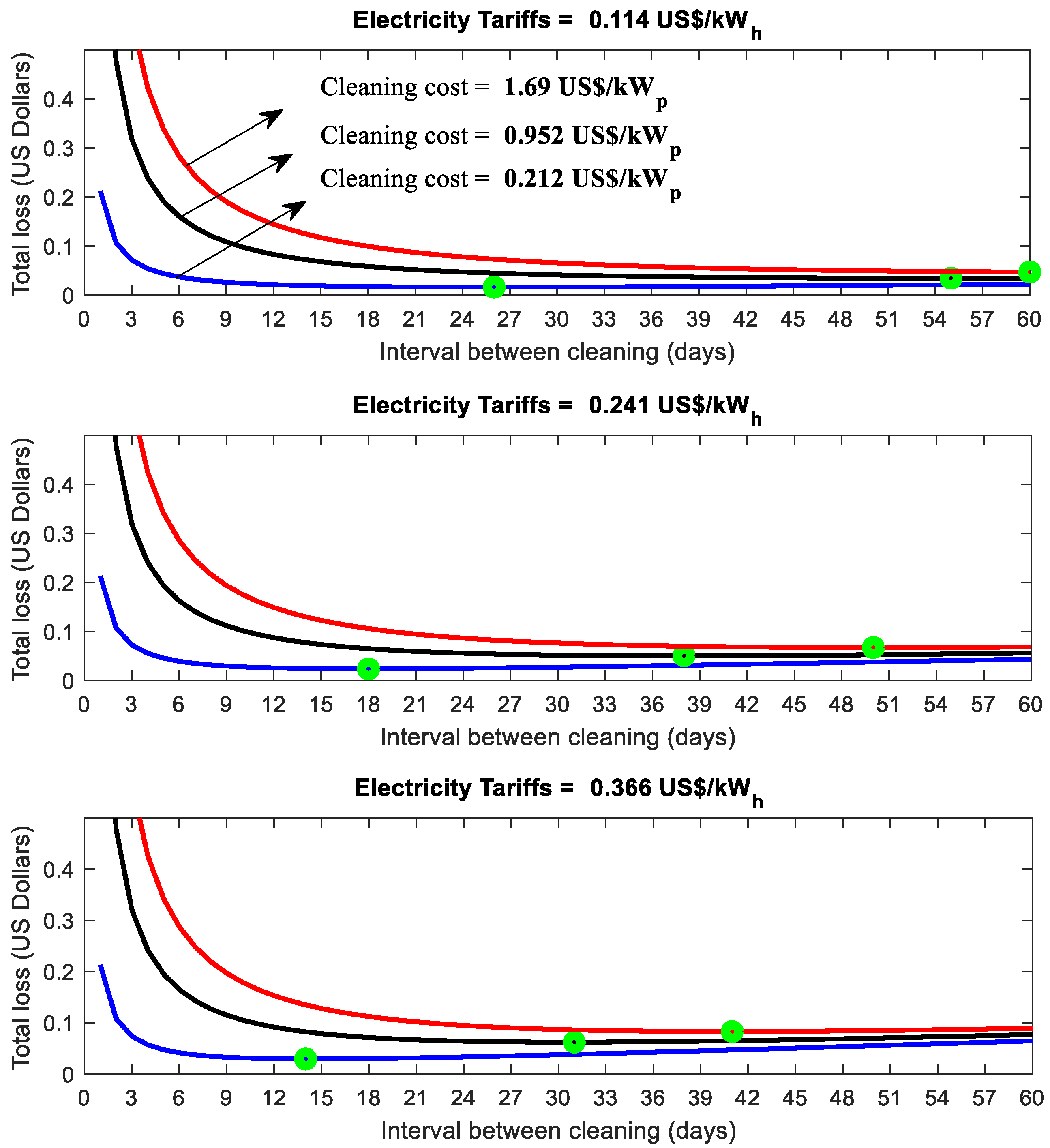
5.3. Investigation of Different Scenarios (Sensitivity Analysis)

In this section, a sensitivity analysis is carried out to investigate the impact of different economic conditions, i.e., different cleaning costs obtained by different PV cleaning mechanisms and different electricity tariffs proposed for different sectors in Jordan, on the optimal cleaning frequency of the PV system under study.

To this end,

Table 3. Cleaning costs and electricity tariffs for the universities sector in Jordan.

	Price	Description
Electricity tariffs (US$/kWh)	0.114	Small industrial companies
	0.241	Commercial companies
	0.366	Residential buildings
Cleaning costs (US$/kWp)	0.212	Wet cleaning with simple tools for ground-mounted or roof-top systems (easy access)
	0.952	Wet cleaning with simple machinery (moderate access)
	1.690	Wet cleaning with cranes and vehicles for solar car parking and solar canopies (difficult access)

reports three different cleaning costs and three different electricity tariffs. Therefore, nine possible combinations of these economic conditions are examined.

Figure 10 shows the average daily losses due to the different cleaning costs (inversely proportional curves) and the dust accumulations (linear curves) obtained by the optimized ELM models when the three different electricity tariffs are used.

Figure 11 shows the total average daily losses together with the optimal cleaning frequency (circles) obtained for the nine different scenarios of cleaning costs and dust accumulations.

The optimal cleaning frequency of each scenario is reported in

Table 4. Optimal cleaning frequency of each scenario.

Scenario [Electricity Tariff, Cleaning Cost]	Optimal Cleaning Frequency (days)
[0.114, 0.212]	26
[0.114, 0.952]	55
[0.114, 1.69]	60
[0.241, 0.212]	18
[0.241, 0.952]	38
[0.241, 1.69]	50
[0.366, 0.212]	14
[0.366, 0.952]	31
[0.366, 1.69]	41

. One can notice the following:

• As the cleaning cost increases, the optimum cleaning frequency increases, at the same electricity tariffs;
• As the electricity tariffs increase, the optimum cleaning frequency decreases at the same cleaning cost.

6. Conclusions

Optimized artificial neural network and extreme learning machine models are used to predict PV system performance under different conditions of actual dust accumulation and ambient temperature that were collected during this study. An experimental data set was collected and analyzed over almost half a year, starting on 17 March and ending on 24 September 2014. The two proposed models managed to predict the PV conversion efficiency as a function of the dust accumulation and the ambient temperature along with jumps in performance when cleaning occurs either by rainfall or manually. It was found that the optimized ELM model predicts the PV performance with a better accuracy compared to the optimized ANN model. It was found that the R² is 91.42% for the ELM model and 90.69% for the ANN model. Moreover, this work serves as an important tool for designers, researchers, operators and stakeholders because it suggests a methodology to predict reductions in PV conversion efficiency due to dust accumulation and ambient temperature along with the optimum cleaning frequency for desert and semi-arid regions in general and in Jordan and the MENA region in particular. For the period considered in this study, it was found that the average daily efficiency reductions were 0.593%/day and 0.615%/day using optimized ANN and ELM models, respectively. These are equivalent to an energy loss of 7.862 and 8.329 kWh/m², which corresponds to an energy loss due to dust accumulation of 0.789 and 0.836 US$/day, employing optimized ANN and ELM models, respectively. Additionally, this paper provides recommendations related to the optimal cleaning intervals, and it was found that the optimal cleaning interval by the optimized ELM model is 14 days, while an optimum cleaning interval of 15 days was obtained using the optimum ANN model. These recommendations take into consideration the cleaning cost and the cost loss due to dust accumulation and the electricity tariff.

References

1. Pillai, U. Drivers of Cost Reduction in Solar Photovoltaics. Energy Econ. 2015, 50, 286–293. [Google Scholar] [CrossRef]
2. Strupeit, L.; Neij, L. Cost Dynamics in the Deployment of Photovoltaics: Insights from the German Market for Building-Sited Systems. Renew. Sustain. Energy Rev. 2017, 69, 948–960. [Google Scholar] [CrossRef]
3. Tanaka, T.Y.; Chiba, M. A Numerical Study of the Contributions of Dust Source Regions to the Global Dust Budget. Glob. Planet. Chang. 2006, 52, 88–104. [Google Scholar] [CrossRef]
4. Tanaka, T.Y.; Kurosaki, Y.; Chiba, M.; Matsumura, T.; Nagai, T.; Yamazaki, A.; Uchiyama, A.; Tsunematsu, N.; Kai, K. Possible Transcontinental Dust Transport from North Africa and the Middle East to East Asia. Atmos. Environ. 2005, 39, 3901–3909. [Google Scholar] [CrossRef]
5. Costa, S.C.S.; Diniz, A.S.A.C.; Kazmerski, L.L. Dust and Soiling Issues and Impacts Relating to Solar Energy Systems: Literature Review Update for 2012–2015. Renew. Sustain. Energy Rev. 2016, 63, 33–61. [Google Scholar] [CrossRef]
6. Mani, M.; Pillai, R. Impact of Dust on Solar Photovoltaic (PV) Performance: Research Status, Challenges and Recommendations. Renew. Sustain. Energy Rev. 2010, 14, 3124–3131. [Google Scholar] [CrossRef]
7. Sarver, T.; Al-Qaraghuli, A.; Kazmerski, L.L. A Comprehensive Review of the Impact of Dust on the Use of Solar Energy: History, Investigations, Results, Literature, and Mitigation Approaches. Renew. Sustain. Energy Rev. 2013, 22, 698–733. [Google Scholar] [CrossRef]
8. Meral, M.E.; Diner, F. A Review of the Factors Affecting Operation and Efficiency of Photovoltaic Based Electricity Generation Systems. Renew. Sustain. Energy Rev. 2011, 15, 2176–2184. [Google Scholar] [CrossRef]
9. Figgis, B.; Ennaoui, A.; Ahzi, S.; Rémond, Y. Review of PV Soiling Particle Mechanics in Desert Environments. Renew. Sustain. Energy Rev. 2017, 76, 872–881. [Google Scholar] [CrossRef]
10. Picotti, G.; Borghesani, P.; Cholette, M.E.; Manzolini, G. Soiling of Solar Collectors—Modelling Approaches for Airborne Dust and Its Interactions with Surfaces. Renew. Sustain. Energy Rev. 2018, 81, 2343–2357. [Google Scholar] [CrossRef]
11. Raza, M.Q.; Nadarajah, M.; Ekanayake, C. On Recent Advances in PV Output Power Forecast. Sol. Energy 2016, 136, 125–144. [Google Scholar] [CrossRef]
12. Madeti, S.R.; Singh, S.N. Monitoring System for Photovoltaic Plants: A Review. Renew. Sustain. Energy Rev. 2017, 67, 1180–1207. [Google Scholar] [CrossRef]
13. Mekhilef, S.; Saidur, R.; Kamalisarvestani, M. Effect of Dust, Humidity and Air Velocity on Efficiency of Photovoltaic Cells. Renew. Sustain. Energy Rev. 2012, 16, 2920–2925. [Google Scholar] [CrossRef]
14. Saidan, M.; Albaali, A.G.; Alasis, E.; Kaldellis, J.K. Experimental Study on the Effect of Dust Deposition on Solar Photovoltaic Panels in Desert Environment. Renew. Energy 2016, 92, 499–505. [Google Scholar] [CrossRef]
15. Kaldellis, J.K.; Kapsali, M. Simulating the Dust Effect on the Energy Performance of Photovoltaic Generators Based on Experimental Measurements. Energy 2011, 36, 5154–5161. [Google Scholar] [CrossRef]
16. Abed, A.M.; Al Kuisi, M.; Khair, H.A. Characterization of the Khamaseen (Spring) Dust in Jordan. Atmos. Environ. 2009, 43, 2868–2876. [Google Scholar] [CrossRef]
17. Mohamed, A.O.; Hasan, A. Effect of Dust Accumulation on Performance of Photovoltaic Solar Modules in Sahara Environment. J. Basic Appl. Sci. Res. 2012, 2, 11030–11036. [Google Scholar]
18. Skoplaki, E.; Palyvos, J.A. On the Temperature Dependence of Photovoltaic Module Electrical Performance: A Review of Efficiency/Power Correlations. Sol. Energy 2009, 83, 614–624. [Google Scholar] [CrossRef]
19. Kim, J.P.; Lim, H.; Song, J.H.; Chang, Y.J.; Jeon, C.H. Numerical Analysis on the Thermal Characteristics of Photovoltaic Module with Ambient Temperature Variatio. Sol. Energy Mater. Sol. Cells 2011, 95, 404–407. [Google Scholar] [CrossRef]
20. Ali, A.H.H.; ElDin, A.S.; Abdel-Gaie, S.M. Effect of Dust and Ambient Temperature on PV Panels Performance in Egypt. Jordan J. Phys. 2015, 8, 113–124. [Google Scholar]
21. Kaushik, S.C.; Rawat, R.; Manikandan, S. An Innovative Thermodynamic Model for Performance Evaluation of Photovoltaic Systems: Effect of Wind Speed and Cell Temperature. Energy Convers. Manag. 2017, 136, 152–160. [Google Scholar] [CrossRef]
22. Al Hanai, T.; Hashim, R.B.; El Chaar, L.; Lamont, L.A. Environmental Effects on a Grid Connected 900 W Photovoltaic Thin-Film Amorphous Silicon System. Renew. Energy 2011, 36, 2615–2622. [Google Scholar] [CrossRef]
23. Pulipaka, S.; Kumar, R. Power Prediction of Soiled PV Module with Neural Networks Using Hybrid Data Clustering and Division Techniques. Sol. Energy 2016, 133, 485–500. [Google Scholar] [CrossRef]
24. Pulipaka, S.; Mani, F.; Kumar, R. Modeling of Soiled PV Module with Neural Networks and Regression Using Particle Size Composition. Sol. Energy 2016, 123, 116–126. [Google Scholar] [CrossRef]
25. Massi Pavan, A.; Mellit, A.; De Pieri, D.; Kalogirou, S.A. A Comparison between BNN and Regression Polynomial Methods for the Evaluation of the Effect of Soiling in Large Scale Photovoltaic Plants. Appl. Energy 2013, 108, 392–401. [Google Scholar] [CrossRef]
26. Mani, F.; Pulipaka, S.; Kumar, R. Characterization of Power Losses of a Soiled PV Panel in Shekhawati Region of India. Sol. Energy 2016, 131, 96–106. [Google Scholar] [CrossRef]
27. Pulipaka, S.; Kumar, R. Analysis of Irradiance Losses on a Soiled Photovoltaic Panel Using Contours. Energy Convers. Manag. 2016, 115, 327–336. [Google Scholar] [CrossRef]
28. Ramli, M.A.M.; Prasetyono, E.; Wicaksana, R.W.; Windarko, N.A.; Sedraoui, K.; Al-Turki, Y.A. On the Investigation of Photovoltaic Output Power Reduction Due to Dust Accumulation and Weather Conditions. Renew. Energy 2016, 99, 836–844. [Google Scholar] [CrossRef]
29. Darwish, Z.A.; Kazem, H.A.; Sopian, K.; Al-Goul, M.A.; Alawadhi, H. Effect of Dust Pollutant Type on Photovoltaic Performance. Renew. Sustain. Energy Rev. 2015, 41, 735–744. [Google Scholar] [CrossRef]
30. Jones, R.K.; Baras, A.; Al Saeeri, A.; Al Qahtani, A.; Al Amoudi, A.O.; Al Shaya, Y.; Alodan, M.; Al-Hsaien, S.A. Optimized Cleaning Cost and Schedule Based on Observed Soiling Conditions for Photovoltaic Plants in Central Saudi Arabia. IEEE J. Photovolt. 2016, 6, 1–9. [Google Scholar] [CrossRef]
31. Guan, Y.; Zhang, H.; Xiao, B.; Zhou, Z.; Yan, X. In-Situ Investigation of the Effect of Dust Deposition on the Performance of Polycrystalline Silicon Photovoltaic Modules. Renew. Energy 2017, 101, 1273–1284. [Google Scholar] [CrossRef]
32. Ghosh, S.; Yadav, V.K.; Mukherjee, V.; Yadav, P. Evaluation of Relative Impact of Aerosols on Photovoltaic Cells through Combined Shannon’s Entropy and Data Envelopment Analysis (DEA). Renew. Energy 2017, 105, 344–353. [Google Scholar] [CrossRef]
33. Koehl, M.; Hoffmann, S. Impact of Rain and Soiling on Potential Induced Degradation. Prog. Photovolt. Res. Appl. 2016, 24, 1304–1309. [Google Scholar] [CrossRef]
34. Hegazy, A.A. Effect of Dust Accumulation on Solar Transmittance through Glass Covers of Plate-Type Collectors. Renew. Energy 2001, 22, 525–540. [Google Scholar] [CrossRef]
35. Mathiak, G.; Hansen, M.; Schweiger, M.; Rimmelspacher, L.; Herrmann, W.; Althaus, J.; Reil, F. PV Module Test for Arid Climates Including Sand Storm and Dust Testing. In Proceedings of the 32nd European Photovoltaic Solar Energy Conference and Exhibition, Munich, Germany, 20–24 June 2016. [Google Scholar]
36. Moharram, K.A.; Abd-Elhady, M.S.; Kandil, H.A.; El-Sherif, H. Influence of Cleaning Using Water and Surfactants on the Performance of Photovoltaic Panels. Energy Convers. Manag. 2013, 68, 266–272. [Google Scholar] [CrossRef]
37. Fathi, M.; Abderrezek, M.; Friedrich, M. Reducing Dust Effects on Photovoltaic Panels by Hydrophobic Coating. Clean Technol. Environ. Policy 2017, 19, 577–585. [Google Scholar] [CrossRef]
38. Maghami, M.R.; Hizam, H.; Gomes, C.; Radzi, M.A.; Rezadad, M.I.; Hajighorbani, S. Power Loss Due to Soiling on Solar Panel: A Review. Renew. Sustain. Energy Rev. 2016, 59, 1307–1316. [Google Scholar] [CrossRef]
39. Guo, B.; Javed, W.; Figgis, B.W.; Mirza, T. Effect of Dust and Weather Conditions on Photovoltaic Performance in Doha, Qatar. In Proceedings of the 2015 1st Workshop on Smart Grid and Renewable Energy, Doha, Qatar, 22–23 March 2015. [Google Scholar]
40. Al Shehri, A.; Parrott, B.; Carrasco, P.; Al Saiari, H.; Taie, I. Impact of Dust Deposition and Brush-Based Dry Cleaning on Glass Transmittance for PV Modules Applications. Sol. Energy 2016, 135, 317–324. [Google Scholar] [CrossRef]
41. Jiang, Y.; Lu, L.; Lu, H. A Novel Model to Estimate the Cleaning Frequency for Dirty Solar Photovoltaic (PV) Modules in Desert Environment. Sol. Energy 2016, 140, 236–240. [Google Scholar] [CrossRef]
42. Sayyah, A.; Horenstein, M.N.; Mazumder, M.K. Energy Yield Loss Caused by Dust Deposition on Photovoltaic Panels. Sol. Energy 2014, 107, 576–604. [Google Scholar] [CrossRef]
43. Abdeen, E.; Orabi, M.; Hasaneen, E.S. Optimum Tilt Angle for Photovoltaic System in Desert Environment. Sol. Energy 2017, 155, 267–280. [Google Scholar] [CrossRef]
44. Mejia, F.A.; Kleissl, J. Soiling Losses for Solar Photovoltaic Systems in California. Sol. Energy 2013, 95, 357–363. [Google Scholar] [CrossRef]
45. Mejia, F.; Kleissl, J.; Bosch, J.L. The Effect of Dust on Solar Photovoltaic Systems. Energy Procedia 2013, 49, 2370–2376. [Google Scholar] [CrossRef]
46. Benatiallah, A.; Mouly Ali, A.; Abidi, F.; Benatiallah, D.; Harrouz, A.; Mansouri, I. Experimental Study of Dust Effect in Mult-Crystal PV Solar Module. Int. J. Multidiscip. Sci. Eng. 2012, 3, 1–4. [Google Scholar]
47. Huang, G.-B.; Zhu, Q.; Siew, C. Extreme Learning Machine: Theory and Applications. Neurocomputing 2006, 70, 489–501. [Google Scholar] [CrossRef]
48. Hu, Z.; Ma, J.; Yang, L.; Li, X.; Pang, M. Decomposition-Based Dynamic Adaptive Combination Forecasting for Monthly Electricity Demand. Sustainability 2019, 11, 1272. [Google Scholar] [CrossRef]
49. Siniscalchi, S.M.; Salerno, V.M. Adaptation to New Microphones Using Artificial Neural Networks with Trainable Activation Functions. IEEE Trans. Neural Netw. Learn. Syst. 2017, 28, 1959–1965. [Google Scholar] [CrossRef]
50. Esteva, A.; Kuprel, B.; Novoa, R.A.; Ko, J.; Swetter, S.M.; Blau, H.M.; Thrun, S. Dermatologist-Level Classification of Skin Cancer with Deep Neural Networks. Nature 2017, 542, 115–118. [Google Scholar] [CrossRef] [PubMed]
51. Salerno, M.V.; Rabbeni, G. An Extreme Learning Machine Approach to Effective Energy Disaggregation. Electronics 2018, 7, 235. [Google Scholar] [CrossRef]
52. Zhou, J.; Yu, X.; Jin, B. Short-Term Wind Power Forecasting: A New Hybrid Model Combined Extreme-Point Symmetric Mode Decomposition, Extreme Learning Machine and Particle Swarm Optimization. Sustainability 2018, 10, 3202. [Google Scholar] [CrossRef]
53. Guerrero-Martinez, J.F.; Frances-Villora, J.V.; Bataller-Mompean, M.; Barrios-Aviles, J.; Rosado-Muñoz, A. Moving Learning Machine towards Fast Real-Time Applications: A High-Speed FPGA-Based Implementation of the OS-ELM Training Algorithm. Electronics 2018, 7, 308. [Google Scholar]
54. Hammad, B.; Al-Abed, M.; Al-Ghandoor, A.; Al-Sardeah, A.; Al-Bashir, A. Modeling and Analysis of Dust and Temperature Effects on Photovoltaic Systems’ Performance and Optimal Cleaning Frequency: Jordan Case Study. Renew. Sustain. Energy Rev. 2018, 82, 2218–2234. [Google Scholar] [CrossRef]
55. ABB. PVI-6.0-TL PVI-8.0-TL General Specifications Outdoor Models; ABB: Zürich, Switzerland, 2013. [Google Scholar]
56. International Electrotechnical Commission (IEC). Photovoltaic System Performance Monitoring—Guidelines for Measurements, Data Exchange and Analysis (IEC 61724); International Electrotechnical Commission (IEC): Geneva, Switzerland, 1998. [Google Scholar]
57. Charabi, Y.; Gastli, A. Integration of Temperature and Dust Effects in Siting Large PV Power Plant in Hot Arid Area. Renew. Energy 2013, 57, 635–644. [Google Scholar] [CrossRef]
58. Menoufi, K. Dust Accumultion on the Surface of Photovoltaic Panels: Introducing the Photovoltaic Soiling Index (PVSI). Sustainability 2017, 9, 963. [Google Scholar] [CrossRef]
59. Erdenedavaa, P.; Rosato, A.; Adiyabat, A.; Akisawa, A.; Sibilio, S.; Ciervo, A. Model Analysis of Solar Thermal System with the Effect of Dust Deposition on the Collectors. Energies 2018, 11, 1795. [Google Scholar] [CrossRef]
60. Rumelhart, D.E.; Hinton, G.E.; Williams, R.J. Learning Representations by Back-Propagating Errors. Nature 1986, 323, 533–536. [Google Scholar] [CrossRef]
61. Hornik, K.; Stinchcombe, M.; White, H. Multilayer Feedforward Networks Are Universal Approximators. Neural Netw. 1989, 2, 359–366. [Google Scholar] [CrossRef]
62. Webb, A.R. Statistical Pattern Recognition; John Wiley & Sons, Ltd.: Hoboken, NJ, USA, 2003. [Google Scholar]
63. Al-Dahidi, S.; Ayadi, O.; Adeeb, J.; Alrbai, M.; Qawasmeh, R.B. Extreme Learning Machines for Solar Photovoltaic Power Predictions. Energies 2018, 11, 2725. [Google Scholar] [CrossRef]
64. Adinoyi, M.J.; Said, S.A.M. Effect of Dust Accumulation on the Power Outputs of Solar Photovoltaic Modules. Renew. Energy 2013, 60, 633–636. [Google Scholar] [CrossRef]
Figure 1. A 7.98 kWp photovoltaic (PV) system installed at the Hashemite University, Zarqa, Jordan before and after cleaning (all 28 modules in the foreground were cleaned manually on 24 September 2014. Modules in the background are not part of this study).
Applsci 09 01397 g001
Figure 2. The dust accumulation (in terms of days of exposure) (top), the average daily ambient temperature (middle), and the daily system conversion efficiency (bottom), for the whole study period of n = 179 data points.
Applsci 09 01397 g002
Figure 3. The artificial neural network (ANN) architecture with two inputs, one hidden layer, and one output.
Applsci 09 01397 g003
Figure 4. The influence of the number of hidden neurons on the prediction performance of the ANN model.
Applsci 09 01397 g004
Figure 5. The influence of the number of hidden neurons on the prediction performance of the extreme learning machine (ELM) model.
Applsci 09 01397 g005
Figure 6. Measured and predicted values of the PV daily system conversion efficiency obtained by the prediction models for the whole study period.
Applsci 09 01397 g006
Figure 7. Measured and predicted values of the PV daily system conversion efficiency obtained by the prediction models for the whole study period, without the dust effect.
Applsci 09 01397 g007
Figure 8. Average daily losses due to cleaning cost (inversely proportional curve) and losses due to dust accumulation (linear curves) obtained by the four prediction models.
Applsci 09 01397 g008
Figure 9. Total average daily losses due to cleaning cost and dust accumulation.
Applsci 09 01397 g009
Figure 10. Average daily losses due to the three different cleaning costs (inversely proportional curves) and the dust accumulation (linear curves) obtained by the optimized ELM model when the three different electricity tariffs are used.
Applsci 09 01397 g010
Figure 11. Total average daily losses together with the optimal cleaning frequency (circles) obtained for the nine different combinations of cleaning costs and dust accumulation.
Applsci 09 01397 g011