Two-Level Attentions and Grouping Attention Convolutional Network for Fine-Grained Image Classification

Abstract

The focus of fine-grained image classification tasks is to ignore interference information and grasp local features. This challenge is what the visual attention mechanism excels at. Firstly, we have constructed a two-level attention convolutional network, which characterizes the object-level attention and the pixel-level attention. Then, we combine the two kinds of attention through a second-order response transform algorithm. Furthermore, we propose a clustering-based grouping attention model, which implies the part-level attention. The grouping attention method is to stretch all the semantic features, in a deeper convolution layer of the network, into vectors. These vectors are clustered by a vector dot product, and each category represents a special semantic. The grouping attention algorithm implements the functions of group convolution and feature clustering, which can greatly reduce the network parameters and improve the recognition rate and interpretability of the network. Finally, the low-level visual features and high-level semantic information are merged by a multi-level feature fusion method to accurately classify fine-grained images. We have achieved good results without using pre-training networks and fine-tuning techniques.

1. Introduction

Fine-grained image classification is an important branch in the field of computer vision [1,2,3,4,5]. The attribute of “large differences within the class and small differences between classes” determines that it is a difficult problem. Compared with traditional image classification, fine-grained image classification has more realistic significance and research value. Positioning local visual differences with sufficient discrimination and fully learning their subtle features is the key to completing fine-grained image classification. The continuous development of machine learning, especially deep learning, provides a means for fine-grained image classification.

The fine-grained image classification model can be divided into strong supervised classification models [6,7,8,9] and weakly supervised classification models [10,11,12,13]. A strong supervised classification model uses additional manual annotation information, in addition to the category labels of the images. Different from the strong supervised classification model, a weakly supervised classification model relies entirely on the algorithm itself to perform the detection of objects and local regions. The powerful feature extraction capabilities of convolutional neural networks (CNNs) [14,15,16] play an important role in this process. Fine-grained image classification requires tracking and learning object-level and part-level features. It makes it easy for us to associate it with visual attention models. The commonly-used attention models are divided into two types: bottom-up attention models [17,18,19] and top-down attention models [20,21,22]. In addition, the visual system theory proves that the left hemisphere of the human brain is better at characterizing local information, while the right hemisphere is better at characterizing the overall information. This provides us with an idea to improve CNNs.

In recent years, the attention model based on convolutional neural networks [23,24,25] has gradually become a common means. We propose a network structure with a two-level attention model, where one branch describes object-level attention and the other branch characterizes pixel-level attention. At the same time, we propose a clustering-based grouping attention mechanism to achieve part-level attention of images by clustering feature channels. In addition, we also consider the combination of low-level visual features and high-level semantic information of the network to express image information. The entire network better accomplishes fine-grained image classification tasks by extracting and learning these more efficient multi-level attention features.

2. Related Work

2.1. Two-Level Attention Model

The attention mechanism has the ability to pay attention to something, while ignoring something else. The ITTI model [26] introduced the attention mechanism for the first time, where it was used for saliency detection. Dzmitry [27] employed a single-layer Attention Model to solve the problem of machine translation. The Inception series [28,29,30] expanded the width of the CNNs to achieve adaptability to different convolutional scales. B-CNN [31] simulates two pathways of the visual nervous system, trying to combine two different features through pair-wise feature interaction. Various improved models of it [32,33] aimed to reduce the computational complexity of the network by reducing the feature dimension. Wang [34] proposed a Second-Order Response Transform (SORT) method, which added an element-based product transformation to the linear sum of dual-branch module. Based on the above research on attention models and multi-branch network structures, we build a two-level attentional block (TA-block). Inspired by the channel attention model [23,25], we combine feature recalibration, based on self-learning, and channel importance representation, based on global pooling, to focus on object-level attention. Inspired by the spatial attention model [24,25], we aggregate the self-learning pixel scoring mechanism and the spatial importance representation, based on channel pooling, to focus on pixel-level attention. Then, we adopt the SORT method to fuse the attentions of the two levels. Two-level attention model (TA-model) is connected by multiple TA-blocks.

2.2. Grouping Attention Model

The earliest group convolutional network began with AlexNet [14]. IGCNets [35] first performs a group convolution operation, and then strengthens the relationship between the channels by interleaved group convolution. Xception [36] further treats each channel as a group and performs depth-wise convolution operations. ShuffleNet [37] uses point-wise group convolution and channel shuffle to increase the contact among channels. These methods improve network performance, but do not evaluate similarities among channels. Two-Level Attention [38] performs spectral clustering on the features of each candidate region to obtain N clusters, thereby performing local region detection on the test samples. PDFS-CNN [39] aggregates the filters which have a significant consistent response to a particular pattern to achieve channel clustering. MA-CNN [40] reorders feature channels to generate multiple-component features and learns better fine-grained features from components in a mutually enhanced manner. Relative to CNNs, the Capsule Network [41] learns the hierarchical structure of different parts of the image through different capsule modules. CNNs usually involves a large number of feature channels, in order to learn high-level semantics. In fact, there is inevitably a situation of high similarity in these high-level semantics. The above models form the part-level attention module, through their respective algorithms. These ideas are extremely valuable, but highly computationally complex. Grouping attention models directly cluster these high-level semantics by vector dot product, thereby dividing the feature channels into groups with huge semantic differences. It considers both semantic differences among channels and the complexity of the network.

2.3. Multi-Level Feature Fusion

From the visualization work of some deep CNNs [42,43,44], it can be seen that different levels of convolution features describe object features and their surroundings from different perspectives. How to obtain low-level visual features while taking into account high-level semantic information has become a new breakthrough in image processing. Hariharan et al. [45,46,47] better achieved fine-grained segmentation, object detection, and semantic pixel segmentation by aggregating low-level features with high-level features. Jin et al. [48] proposed using a recurrent neural network to transfer high-level semantic information and low-level spatial features to each other for the analysis of scene images. Based on the two-level attention and grouping attention models, this paper combines the attention features of multiple intermediate layers and delivers them layer-by-layer. The network then learns the high-order information of different levels to provide convolutional features from different perspectives. Finally, we better guide the fine-grained image classification by combining low-level visual features and advanced semantic information.

3. Approach

3.1. Two-Level Attention Model

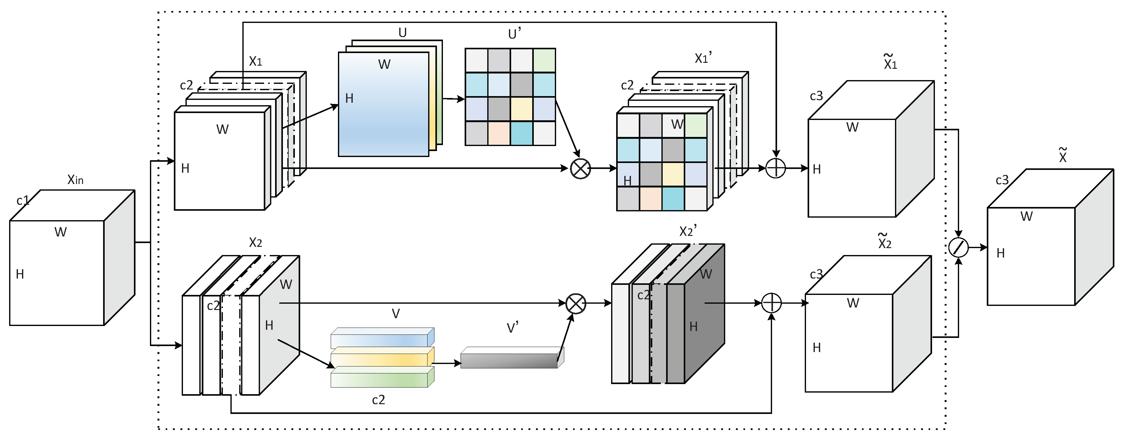
B-CNN [31] obtained a second-order feature representation through a bilinear structure, which makes it advantageous in fine-grained image classification tasks. We embraced this observation and adopted a multi-block two-branch structure model in this study. Combined with the characteristics of fine-grained images, we built a convolutional neural network of the two-level attention model (TA-model). The first branch of each block captures pixel-level attention, and the other branch locks object-level attention. As B-CNN obtains second-order features by multiplying pair-wise feature matrixes, the computational complexity is extremely high. In this paper, the SORT [34] method is used for the two-level attention feature fusion. The TA-block structure is shown in Figure 1.

The dotted box in Figure 1 represents a two-level attention block (TA-block). The TA-model is composed of multiple TA-blocks. The upper half of the dashed box shows pixel-level feature attention, $X_{in}$ represents the input feature maps of TA-model, and $X_1$ is obtained by $X_{in}$ through a convolution operation, where the convolution kernel is $K_a$ = [$K_{a1}$, $K_{a2}$, …, $K_{ac2}$]:

$$X_1=ConV(K_a,X_{in})=\sum _{i=1}^{c2}{K}_{ai}\odot X_{in}$$

(1)

where ⊙ indicates the convolution operation, and the number of feature channels is increased from c1 to c2. Next, U consists of three parts, which integrates the self-learning feature map of LIR-CNN [24] and the maximum and average channel pooling feature maps of CBAM [25]. They are implemented by Equations (2)–(5), respectively.

$$U_1=ConV(K_b,X_1)=K_{b1}\odot X_1$$

(2)

$$U_2=MaxPool(X_1,axis=3)$$

(3)

$$U_3=AvgPool(X_1,axis=3)$$

(4)

$$U=Relu\left(Concat(U_1,U_2,U_3)\right)$$

(5)

where $K_b$ = [$K_{b1}$] shows that there is only one convolution kernel, and the convolution result is a feature map of a single channel. “MaxPool(*)” and “AvgPool(*)”, respectively, represent the max-pooling and average-pooling operations along the feature channel direction (“axis = 3”). The Relu activation function guarantees the non-linearity and sparsity of the network. The “Concat(*)” function means that $U_1$, $U_2$, and $U_3$ are stacked along the feature channel direction.

$$U^{\prime }=Sigmoid\left(ConV(K_c,U)\right)=Sigmoid(K_{c1}\odot U)$$

(6)

where $K_c$ = [$K_{c1}$] is also a single convolution kernel. After the convolution operation, U is activated by the Sigmoid function to obtain a two-dimensional table $U^{\prime }$ with a value range of [0–1]. This table records the importance of each pixel in the image. Then, we multiply this table by the position corresponding to $X_1$, as in Equation (7).

$$X_1^{\prime }=Multiply(U^{\prime },X_1)=U^{\prime }\otimes X_1$$

(7)

$${\tilde{X}}_1=Add(X_1^{\prime },X_1)=X_1^{\prime }\oplus X_1$$

(8)

where ⊗ indicates that the corresponding position of each feature channel is multiplied by $U^{\prime }$, and $X_1^{\prime }$ is the feature map after being processed by the pixel-level attention. As the ResNet structure is used in this paper, ${\tilde{X}}_1$ is obtained by adding the corresponding positions of $X_1$ and $X_1^{\prime }$, where ⊕ indicates matrix addition.

The lower half of the dashed box indicates the object-level features. First, we calculate the importance of each feature channel for the final classification result, and then assign these importance factors to the corresponding feature channels. Finally, according to the design of the ResNet structure, we sum the feature maps before and after the TA-model processing. Equations (9)–(16) illustrate the steps to achieve this process.

$$X_2=ConV(K_d,X)=\sum _{i=1}^{c2}{K}_{di}\odot X$$

(9)

where ⊙ denotes a convolution operation, and $K_d$ is a convolution kernel of X to X2: $K_d$ = [$K_{d1}$, $K_{d2}$, …, $K_{dc2}$].

$$V_1=DWConV(K_e,X_2)=\sum _{i=1}^{c2}(K_{ei}\odot X_{2i})$$

(10)

$$V_2=GlobleMaxPool\left(X_2\right)$$

(11)

$$V_3=GlobleAvgPool\left(X_2\right)$$

(12)

$$V=Relu\left(Concat(V_1,V_2,V_3)\right)$$

(13)

where “DWConV” means depth-wish convolution [41], and $K_e$ is the convolution kernel of $X_2$ to $V_1$, $K_e$ = [$K_{e1}$, $K_{e2}$, …, $K_{ec2}$], where the number of channels of the convolution kernel is 1. “GlobleMaxPool” and “GlobleAvgPool” represent global max-pooling and global average-pooling, respectively. Finally, $V_1$, $V_2$, and $V_3$ are connected in series along the direction of the feature channel and activated by the Relu function to obtain V.

$$V^{\prime }=Sigmoid\left(ConV(K_f,V)\right)=Sigmoid(K_{f1}\odot V)$$

(14)

After the convolution and activation operations, V obtains the vector $V^{\prime }$ that characterizes the importance of the feature channels. The convolution kernel is $K_f$ ($K_f$ = [$K_{f1}$]) and the activation function is Relu.

$$X_2^{\prime }=Multiply(V^{\prime },X_2)=V^{\prime }\otimes X_2$$

(15)

$${\tilde{X}}_2=Add(X_2^{\prime },X_2)=X_2^{\prime }\oplus X_2$$

(16)

where $X_2^{\prime }$ is obtained by multiplying all values of each feature channel by an important factor, and this operation is described by ⊗. The ⊕ operation indicates that the positions corresponding to $V^{\prime }$ and $X_2$ are summed.

$$\tilde{X}={\tilde{X}}_1\oslash {\tilde{X}}_2={\tilde{X}}_1+{\tilde{X}}_2+\sqrt{Relu\left({\tilde{X}}_1\right)\otimes Relu\left({\tilde{X}}_2\right)+\epsilon }$$

(17)

Equation (17) implements the feature fusion of the two attention branches. The ⊘ sign indicates that the feature fusion is performed using the SORT method. Here, the Relu function can be used to avoid negative numbers in the square root, and take the offset $\epsilon$ = 0.0001. After TA-model processing, $X_{in}$ is convoluted into $\tilde{X}$, with a certain high level of semantics.

3.2. Grouping Attention Model

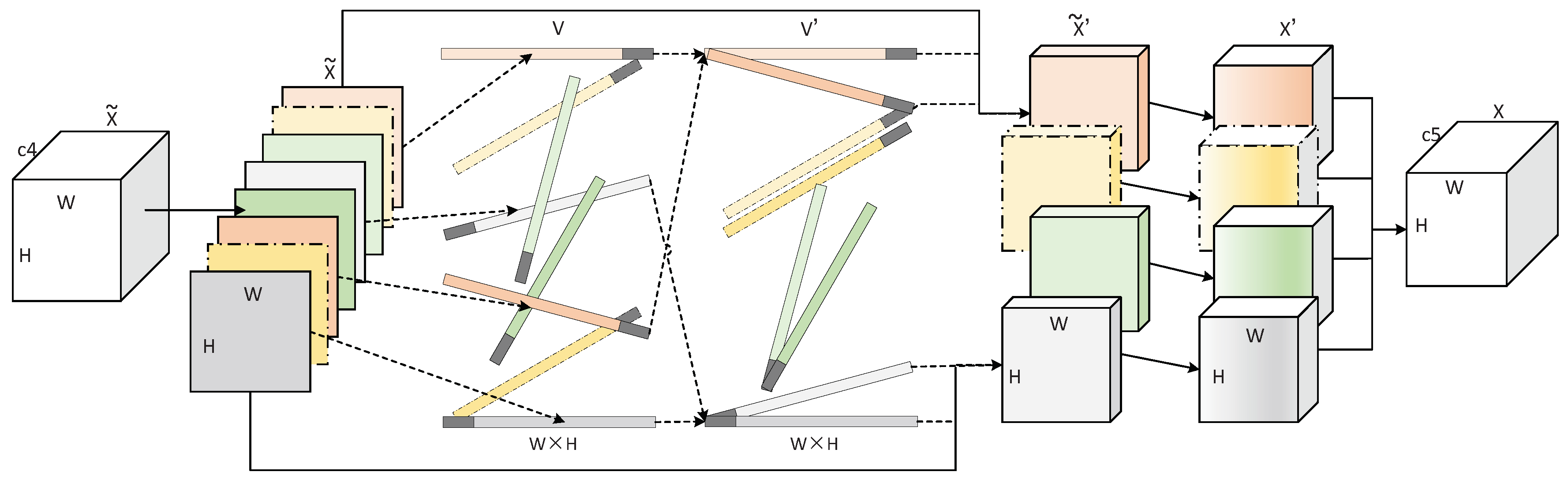
The lower layers of the CNN handle low-level visual features, while the higher layers process high-level semantic information. The feature maps ($\tilde{X}$) acquired by the TA-model processing in Section 3.1 already have high semantic features. Each of its feature channels denotes semantics with a certain local meaning in the image. In this section, we further group these semantics into an attention model with local characterization. The structure diagram of the grouping attention model (GA-model) is shown in Figure 2.

As shown in Figure 2, $\tilde{X}$ is obtained by a TA-block, and then we process each feature channel of $\tilde{X}$. V is a set of vectors that are stretched by $\tilde{X}$. The gray head represents the direction of the vector, and the length of the vector is “W×H”. Next, we perform a dot product on the vectors. The dot product result of the two vectors is a scalar value. The larger the value, the higher the similarity between the two vectors, and vice versa. With vector dot products, we group vectors with high similarity into a class to better represent local semantics. $V^{\prime }$ is a clustered vector set, and we rearrange $\tilde{X}$ according to the order of this set to get ${\tilde{X}}^{\prime }$. At this time, $X^{\prime }$ is a plurality of semantic units after grouping attention. Next, a group convolution (GC-block) [35] operation is performed for each semantic unit. In this way, we can execute feature learning for each semantic unit. It is worth mentioning that the group convolution itself can greatly reduce the amount of parameters of the network. Finally, we concatenate multiple semantic units along the feature channel direction to get X. The implementation algorithm of $\tilde{X}$ to ${\tilde{X}}^{\prime }$ is as shown in Algorithm A1 (Appendix A).

3.3. Multi-Level Feature Fusion

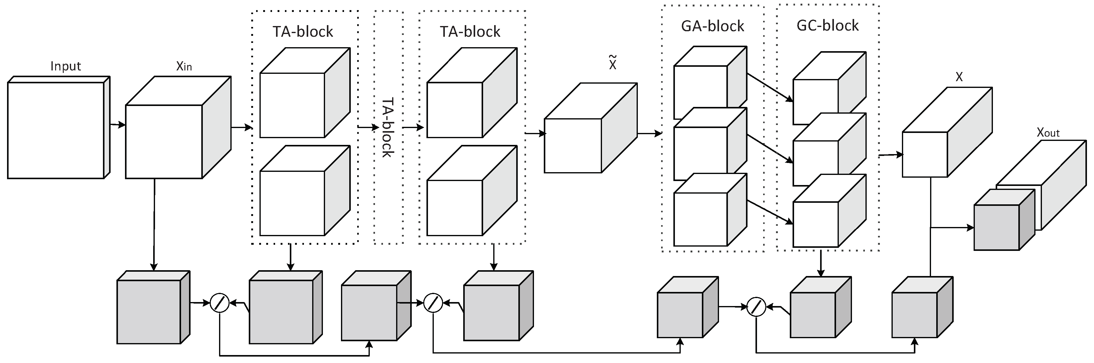
As the number of layers of the CNN increases, the information we obtain gradually evolves from low-level visual features to high-level semantic information. Usually, we only use the semantic features of the last layer for image processing. However, the low-level visual features often retain more spatial structure and detail information. In this section, we have designed a new feature fusion method to ensure that both the low-level visual features and high-level semantic information are fully utilized. We will perform a simple convolution process on each module in the network and combine them with the feature maps on the main path to perform fine-grained image classification. In particular, for our proposed TA-model and GA-model, multi-level feature fusion can fuse information between different branches of each module. For example, we can aggregate the attentions of the two branches of the TA-block, or we can link the grouping attentions of the GC-block. Here, we did not choose to simply sum the high-level information and the low-level features, but use the SORT method to obtain high-order features to improve the non-linearity and robustness of the network. Finally, multi-level feature fusion not only achieves the fusion between low-level visual features and high-level semantic information, but also achieves the combination of local features and overall features. A schematic diagram of multi-level feature fusion is shown in Figure 3.

As shown in Figure 3, the modules in the dashed box are TA-block, GA-block, and GC-block, from left to right. Among them, the TA-model is composed of multiple TA-blocks in series, and GA-model is constituted of GA-block and GC-block. The darker colored modules in the network are convolved by the TA-block and GC-block, respectively. The ⊘ is a SORT operation, which represents high-order information fusion between different hierarchical features. The resulting $X_{out}$ are feature maps for fine-grained image classification. Adding the global pooling module and the dense module to $X_{out}$ is the structure diagram of the entire network implementation.

4. Experiments

4.1. Datasets and Experimental Details

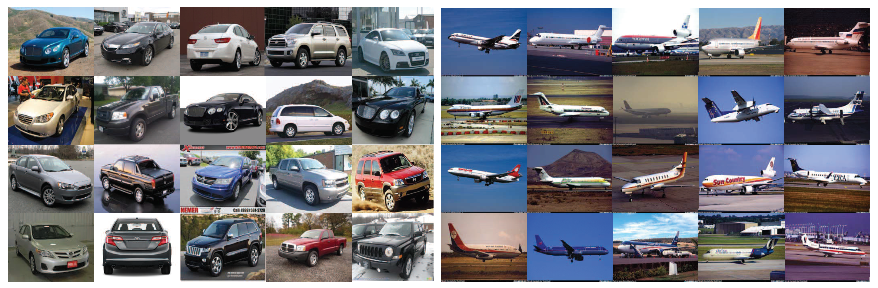
In this section, we perform experiments on two fine-grained image datasets, Stanford Cars [49] and FGVC-Aircraft [50]. The Stanford Cars dataset consists of 16,185 images in 196 categories. This dataset is split into 8144 training images and 8041 test images. The FGVC-Aircraft dataset consists of 10,000 images. They are divided into 100 categories. This dataset includes 6667 training images and 3333 test images. Figure 4 shows partial examples of these two datasets.

The algorithms in this paper are implemented on Keras 2.2.4. The backend of this framework is Tensorflow 1.6.0. In addition, the programming language and version is Python 3.5.2 and the graphics card model is a GeForce GTX 1080. The learning rates of the models were $0.1$, $0.01$, and $0.001$, at 0–150 epochs, 150–190 epochs, and 190–230 epochs. This paper uses convolutional networks with residual structures. Network structures, such as ResNet-50, are not used, mainly because their parameters are too large. This will result in some improved models, based on mainstream residual networks which are difficult to complete in existing experimental environments. The two-level attention and group attention residual network we propose can achieve more accurate feature learning, such that a large number of feature maps are not needed before feature classification. The parameters of Res-CNN and its various improved models are shown in

Table 1. The simple structures of several convolutional networks with residual module.

Model	Conv1	Conv2	Conv3	Conv4	Conv5	Conv6	Dence
Res-CNN	(16,7,3) (16,5,3) (16,3,3)	$\left[\begin{array}{c}64,3,2\\ 64,3,1\\ 64,3,1\end{array}\right]$	$\left[\begin{array}{c}96,3,2\\ 96,3,1\\ 96,3,1\end{array}\right]$	$\left[\begin{array}{c}160,3,2\\ 160,3,1\\ 160,3,1\end{array}\right]$	$\left[\begin{array}{c}192,3,2\\ 192,3,1\\ 192,3,1\end{array}\right]$	$\left[\begin{array}{c}192,3,2\\ 192,3,1\\ 192,3,1\end{array}\right]$	GAP (5,5) Dence (196/100)
	$\left[\begin{array}{c}48,3,1\\ 48,3,1\\ 48,3,1\end{array}\right]$	$\left[\begin{array}{c}64,3,1\\ 64,3,1\\ 64,3,1\end{array}\right]$	$\left[\begin{array}{c}96,3,1\\ 96,3,1\\ 96,3,1\end{array}\right]$	$\left[\begin{array}{c}160,3,1\\ 160,3,1\\ 160,3,1\end{array}\right]$	$\left[\begin{array}{c}192,3,1\\ 192,3,1\\ 192,3,1\end{array}\right]$	$\left[\begin{array}{c}192,3,1\\ 192,3,1\\ \mathrm{bs},3,1\end{array}\right]$
TA-CNN	TA-block	TA-block	TA-block	TA-block	TA-block	TA-block
GA-CNN					GA-block	GC-block
TGA-CNN	TA-block	TA-block	TA-block	TA-block	TA-block	GA-model
MFF	[16,2,2]	$\left[\begin{array}{c}16,1,1\\ 32,2,2\end{array}\right]$	$\left[\begin{array}{c}32,1,1\\ 64,2,2\end{array}\right]$	$\left[\begin{array}{c}64,1,1\\ 96,2,2\end{array}\right]$	$\left[\begin{array}{c}96,1,1\\ 128,2,2\end{array}\right]$	[128,1,1]

.

Res-CNN is the residual network model we defined. Table 1 briefly describes the convolution parameters of several networks based on Res-CNN. Res-CNN consists of six convolutional blocks, a global average pooling layer, and a dense layer. There are three convolution operations in one residual block, in each square bracket. The three parameters of the convolution kernel are the number of feature channels after convolution, the sizes of the convolution kernels, and the strides. $Conv1$ first convolves the input images through three different sizes of convolution kernels to provide feature maps of different fields of view. The upper-half convolution kernels have strides of 3 or 2, to reduce the size of the feature maps. The residual blocks, enclosed in blue square brackets in Table 1, need to be repeated 3 times. TA-CNN is a TA-block module added after each convolution block. GA-CNN is a group attention residual network, which adds a GA-block after $Conv5$ and replaces $Conv6$ with a GC-block. TGA-CNN is a residual network that introduces both TA-model and GA-model, where the GA-model consists of GA-block and GC-block. $MFF$ refers to a multi-level feature fusion method.

4.2. Two-Level Attention Model

The Res-CNN structure is shown in Table 1, where $bs$ in the blue box of $Conv6$ takes 192 in the first two residual blocks and 320 in the last residual block. OARes-CNN embeds an object-level attention module in the Res-CNN structure. PARes-CNN adds a pixel-level attention module to the Res-CNN structure. Their detailed structures are shown in the upper and lower halves of Figure 1. TA-CNN introduces a two-level attention module simultaneously in the Res-CNN structure. For example, in Table 1, convolutional blocks, such as $Conv1$ and $Conv2$, are followed by a TA-block. At the same time, we conducted feature fusion for two levels of attention. TA-CNN_ADD indicates that a summation operation is performed on two-level attention features, and TA-CNN_SORT shows that the SORT method is performed on two-level attention features.

The experimental data shown below was obtained without using pre-training networks and fine-tuning techniques. As shown in

Table 2. The parameters and frames per second (FPS) of the residual networks carrying different attention models, and the classification accuracies of these networks on the two datasets.

Model	Accuracy(%)		Parameters	FPS
	Cars	Aircrafts
B-CNN	83.90	78.40	–	8
Res-CNN	84.29	82.15	14.09M	40
OARes-CNN	84.87	82.65	15.78M	38
PARes-CNN	84.80	82.62	14.10M	38
TA-CNN_ADD	85.10	82.94	15.78M	36
TA-CNN_SORT	85.22	83.01	15.78M	36

, Res-CNN was better, in terms of classification accuracy and time complexity, than B-CNN; due to the use of residual structure, and as Res-CNN does not adopt the local pairwise feature interaction methods, so its number of parameters is also greatly reduced. Compared to Res-CNN, OARes-CNN increased the classification accuracy by $0.58\%$, as we introduced an object-level attention mechanism. PARes-CNN introduced a pixel-level attention mechanism, and achieved similar results. However, single-level attention is not obvious enough to improve network performance. TA-CNN focuses on the classified images by using a two-level attention. TA-CNN_SORT achieved better results than TA-CNN_ADD, as the former learned higher-level feature representations. Here, we define TA-CNN_SORT as TA-CNN. Compared with Res-CNN, the classification accuracies of TA-CNN on the datasets Stanford Cars and FGVC-Aircraft increased by $0.93\%$ and $0.86\%$, respectively. Correspondingly, the network parameters have increased by about $1.69M$, and the time complexity has increased slightly. It is worth mentioning that, without using pre-training conditions, compared with B-CNN, the classification accuracy of TA-CNN increased by 4.61% for the FGVC-Aircraft dataset.

4.3. Grouping Attention Model

The focus of this section is on several grouping attention residual networks. The several convolutional networks in

Table 3. The parameters and FPS of the group attention residual networks, and the classification accuracies of these networks on the two datasets.

Model	Accuracy(%)		Parameters	FPS
	Cars	Aircrafts
Res-CNN	84.29	82.15	14.09M	40
Res-CNN_G4	88.30	86.11	13.40M	30
Res-CNN_G8	89.51	87.06	12.89M	24
Res-CNN_G12	88.15	86.22	12.71M	21
Res-CNN_GX	85.94	83.64	12.53M	38

introduce a group attention model (GA-model) into the Res-CNN architecture. This model consists of a group attention block (GA-block) and a group convolution block (GC-block). Their main structures are shown in GA-CNN in Table 1, and the GA-block operation is executed after $Conv5$; that is, these feature channels with high semantics are divided into multiple groups. As shown in Table 3, we divided them into 1 group, 4 groups, 8 groups, 12 groups, and X groups (X indicates the number of feature channels, and the value in this experiment was 192). Then, we performed a GC-block operation on each group, and the number of feature channels after the group convolution in the experiment was still 192. It should be noted here that replacing $Conv6$ with a GC-block will greatly reduce the network parameters. In order to compare network performance fairly, we performed a traditional convolution operation on the feature maps before group convolution to obtain 128 feature channels. These two types of feature maps were then merged for the final image classification tasks.

Res-CNN treats the feature maps after $Conv5$ as one group, which is Res-CNN_G1. As can be seen from Table 3, as the groups increase, the amount of parameters slowly decreases, while the time complexity increases gradually. This is because when the group convolution operation is performed, the group increases, and the number of channels per group decreases, resulting in a decrease of parameters. The extra time is mainly consumed in the process of grouping. Res-CNN_GX is an exception, and its time complexity is similar to that of Res-CNN, mainly because we adopt depth-wise convolution operations to improve network efficiency. For the Cars and Air datasets, the classification accuracies were the highest in the 8 groups, reaching $89.51\%$ and $87.06\%$, respectively. These show that the two datasets can achieve more accurate classification when obtaining about 8 discriminative local features. In addition, Res-CNN_GX achieved better results than Res-CNN after introducing additional traditional convolution operations. This illustrates that the use of grouping attention at the advanced semantics layer helps us to improve network classification performance. We define Res-CNN_G8 as GA-CNN. Compared with Res-CNN, the classification accuracies of GA-CNN on the datasets Stanford Cars and FGVC-Aircraft increased by 5.22% and 4.91%, respectively.

In the previous experiment, we improved the Res-CNN with a two-level attention model or a grouping attention model, respectively. Naturally, we will embed both two-level attention model and grouping attention model into the Res-CNN architecture; that is, introduce grouping attention on the TA-CNN. As shown in TGA-CNN in Table 1, we replaced $Conv6$ with a GA-model (GA-block and GC-block), and the rest of the operation was the same as mentioned earlier.

TA-CNN is TA-CNN_SORT in Table 2, and the feature maps after $Conv5$ can be interpreted as only one group. TA-CNN_GX indicates that each feature channel of the corresponding feature maps is divided into one group. As TA-CNN_GX employs depth-wise convolution operations, its parameters and time complexity are smaller. As the number of groups increases, the parameters of other group networks are reduced and time complexity is increased. Compared with TA-CNN, the FPS of TA-CNN_G12 is reduced from 40 to 20. As shown in

Table 4. The parameters and FPS of the two-level attentions and group attention residual networks, and the classification accuracies of these networks on the two datasets.

Model	Accuracy(%)		Parameters	FPS
	Cars	Aircrafts
TA-CNN	85.22	83.01	15.78M	36
TA-CNN_G4	89.13	86.55	15.07M	27
TA-CNN_G8	90.32	87.47	14.55M	23
TA-CNN_G12	89.04	86.82	14.38M	20
TA-CNN_GX	86.81	84.69	14.20M	36

, when the number of groups was about 8, the classification accuracies of the Stanford Cars and FGVC-Aircraft datasets were the highest: $90.32\%$ and $87.47\%$, respectively. We define TA-CNN_G8 as TGA-CNN. Compared with TA-CNN, the classification accuracies of TGA-CNN increased by 5.10% and 4.46% for the Stanford Cars and FGVC-Aircraft datasets, respectively. It can be seen, from Table 2 and Table 3, that the grouping attention model has great significance for improving network performance.

4.4. Multi-Level Feature Fusion

In this section, we add the Multi-Level Feature Fusion (MFF) method to the Res-CNN, TA-CNN (TA-CNN_SORT), GA-CNN (Res-CNN_G8), and TGA-CNN (TA-CNN_G8) models, respectively. The parameters of the MFF are as shown in Table 1. The 2 × 2 convolution kernels are used to reduce the feature dimension, and the 1 × 1 convolution kernels are applied to adjust the number of feature channels. This can reduce the network parameters while preserving the features of each layer as much as possible. The MFF method can combine low-level visual features with high-level semantic information. The experimental results are shown in

Table 5. The parameters and FPS of the residual networks with multi-level feature fusion (MFF), and the classification accuracies of these networks on the two datasets.

Model	Accuracy(%)		Parameters	FPS
	Cars	Aircrafts
Res-CNN	84.29	82.15	14.09M	40
Res-CNN_MFF	84.95	82.63	14.77M	36
TA-CNN	85.22	83.01	15.78M	36
TA-CNN_MFF	85.64	83.26	16.44M	34
GA-CNN	89.51	87.06	12.89M	24
GA-CNN_MFF	90.41	87.49	13.01M	24
TGA-CNN	90.32	87.47	14.55M	23
TGA-CNN_MFF	91.05	87.93	14.67M	23

.

As shown in Table 5, after the introduction of the MFF method, the four network structures improved in classification accuracies, which indicates that low-level visual features and high-level semantic information did have an impact on the classification results. Comparing the first four and the last four groups of the experiments (i.e., introduced the network before and after the grouping attention), the parameters of the last four groups decreased, but the time complexity increased accordingly. Meanwhile, the classification accuracies of the latter four groups increased significantly. The parameters of TA-CNN_MFF were up to $16.44M$. Comparing TGA-CNN and GA-CNN_MFF, it can be found that the latter achieved higher classification accuracies under the condition of less parameters and lower time complexity. This illustrates that it is necessary to perform group attention operation in the advanced semantic layers of the network. The classification accuracies of TGA-CNN_MFF on Cars and Air datasets reached $91.05\%$ and $87.93\%$, respectively. This is because we took into account the overall and part attentions, as well as the high-level and low-level features. Its time complexity was also the highest, and the value of FPS was 23. Compared with Res-CNN, with the support of the TA-model, GA-model, and MFF method, the classification accuracy of TGA-CNN_MFF increased by 6.76% and 5.78% on the datasets Stanford Cars and FGVC-Aircraft, respectively.

4.5. Comparisons With Prior Methods

In the previous sections, we evaluate the proposed methods on two datasets: Stanford Cars and FGVC-Aircraft. Now, we compare our results with several other fine-grained classification models, including FV-CNN [51], DVAN [10], Random Maclaurin [32], Tensor Sketch [32], LRBP [33], and MA-CNN [40]. None of these models use bounding box information or part annotation. The classification accuracies of the mentioned methods are shown in

Table 6. The classification accuracies of these models on the two datasets.

Model	Accuracy (%)
	Cars	Aircrafts
FV-CNN	87.79	81.46
DVAN	87.10	–
Random Maclaurin	89.54	87.10
Tensor Sketch	90.19	87.18
LRBP	90.92	87.31
MA-CNN	92.80	89.90
TGA-CNN(Ours)	91.05	87.93

.

Here, TGA-CNN represents the complete model of this paper (i.e., TGA-CNN with the MFF method). Compared to FV-CNN, TGA-CNN’s classification accuracies on Cars and Aircrafts increased by 3.26% and 6.47%, respectively. Similarly, for Cars, the classification accuracy of TGA-CNN was 3.95% higher than DVAN. The Random Maclaurin, Tensor Sketch, and LRBP approaches are all improved versions of B-CNN, and our model was slightly better than these three methods. The classification accuracies of MA-CNN on the two data sets were 1.75% and 1.97% higher than our model, respectively. MA-CNN captures smaller parts by unsupervised part learning approaches. Then, it makes part generation and feature learning mutually reinforcing. This is the method we can learn from.

5. Conclusions

In this paper, we build a new network structure with a multi-level attention model by combining a two-level attention model (TA-model) and a grouping attention model (GA-model). At the same time, we adopt the multi-level feature fusion method for the unified learning of low-level visual features and high-level semantic information of the network. The entire network subtly completes the fine-grained image classification task under small-data conditions by adding attention modules and feature fusion. The proposed structure does not need a bounding box or partial annotation for training, and can be easily embedded into all convolutional networks. The experimental results demonstrate good performance on fine-grained classification. In the future, we will conduct the research in two directions. First, we will use more efficient similarity measurement methods and multi-stage grouping attention to obtain more distinguishing features. Second, we will try to borrow object detection mechanisms to locate and capture more precise fine-grained features.

References

- Li, Y.; Zeng, J.B.; Shan, S.G.; Chen, X.L. Learning Latent Representations of 3D Human Pose with Deep Neural Networks. IEEE Trans. Image Process. 2018, 28, 2439–2450. [Google Scholar] [CrossRef]
- Lu, K.L.; Chu, T.H. An Image-Based Fall Detection System for the Elderly. Appl. Sci. 2018, 8, 1995. [Google Scholar] [CrossRef]
- Liu, J.; Lin, L.; Cai, Z.H.; Wang, J.; Kim, H.J. Deep web data extraction based on visual information processing. J. Ambient. Intell. Humaniz. Comput. 2017, 10, 1–11. [Google Scholar] [CrossRef]
- Katircioglu, I.; Tekin, B.; Salzmann, M.; Lepetit, V.; Fua, P. Occlusion Aware Facial Expression Recognition Using CNN With Attention Mechanism. Int. J. Comput. Vis. 2018, 126, 1326–1341. [Google Scholar] [CrossRef]
- Liu, J.; Gu, C.K.; Wang, J.; Kim, H.J. Multi-scale multi-class conditional generative adversarial network for handwritten character generation. J. Supercomput. 2017, 12, 1–19. [Google Scholar] [CrossRef]
- Berg, T.; Belhumeur, P.N. POOF: Part-Based One-vs.-One Features for Fine-Grained Categorization, Face Verification, and Attribute Estimation. In Proceedings of the IEEE Conference on Computer Vision and Pattern Recognition, Portland, OR, USA, 23–28 June 2013; pp. 955–962. [Google Scholar]
- Huang, S.L.; Xu, Z.; Tao, D.C.; Zhang, Y. Part-Stacked CNN for Fine-Grained Visual Categorization. In Proceedings of the IEEE Conference on Computer Vision and Pattern Recognition, Las Vegas, NV, USA, 26 June–1 July 2016; pp. 1173–1182. [Google Scholar]
- Lin, D.; Shen, X.Y.; Lu, C.W.; Jia, J.Y. Deep LAC: Deep localization, alignment and classification for fine-grained recognition. In Proceedings of the IEEE Conference on Computer Vision and Pattern Recognition, Boston, MA, USA, 8–10 June 2015; pp. 1666–1674. [Google Scholar]
- Zhang, N.; Donahue, J.; Girshick, R.; Darrell, T. Part-based R-CNNs for Fine-grained Category Detection. In Proceedings of the European Conference on Computer Vision, Zurich, Switzerland, 6–12 September 2014; pp. 834–849. [Google Scholar]
- Zhao, B.; Wu, X.; Feng, J.S.; Peng, Q.; Yan, S.C. Diversified Visual Attention Networks for Fine-Grained Object Classification. IEEE Trans. Multimed. 2017, 19, 1245–1256. [Google Scholar] [CrossRef]
- Jaderberg, M.; Simonyan, K.; Zisserman, A.; Kavukcuogu, K. Spatial transformer networks. In Proceedings of the Advances in Neural Information Processing Systems, Montréal, QC, Canada, 7–12 December 2015; pp. 2017–2025. [Google Scholar]
- Wang, Y.M.; Morariu, V.I.; Davis, L.S. Learning a Discriminative Filter Bank within a CNN for Fine-grained Recognition. In Proceedings of the IEEE Computer Vision and Pattern Recognition, Salt Lake City, UT, USA, 19–21 June 2018; pp. 5209–5217. [Google Scholar]
- Wang, D.Q.; Shen, Z.Q.; Shao, J.; Zhang, W.; Xue, X.Y.; Zhang, Z. Multiple Granularity Descriptors for Fine-Grained Categorization. In Proceedings of the IEEE International Conference on Computer Vision, Santiago, Chile, 13–16 December 2015; pp. 2399–2406. [Google Scholar]
- Krizhevsky, A.; Sutskever, I.; Hinton, G. Imagenet classification with deep convolutional neural networks. In Proceedings of the International Conference on Neural Information Processing Systems, Lake Tahoe, NV, USA, 3–6 December 2012; pp. 1097–1105. [Google Scholar]
- Simonyan, K.; Zisserman, A. Very Deep Convolutional Networks for Large-Scale Image Recognition. arXiv 2015, arXiv:1409.1556v6. [Google Scholar]
- He, K.M.; Zhang, X.Y.; Ren, S.Q.; Sun, J. Deep Residual Learning for Image Recognition. In Proceedings of the IEEE Conference on Computer Vision and Pattern Recognition, Las Vegas, NV, USA, 26 June–1 July 2016; pp. 770–778. [Google Scholar]
- Itti, L.; Koch, C. Computational modelling of visual attention. Nat. Rev. Neurosci. 2001, 2, 194–203. [Google Scholar] [CrossRef] [PubMed]
- Itti, L.; Koch, C.; Niebur, E. A model of saliency-based visual attention for rapid scene analysis. IEEE Trans. Pattern Anal. Mach. Intell. 1998, 20, 1254–1259. [Google Scholar] [CrossRef]
- Meur, O.E.; Callet, P.L.; Barba, D.; Thoreau, D. A coherent computational approach to model bottom-up visual attention. IEEE Trans. Pattern Anal. Mach. Intell. 2006, 28, 802–817. [Google Scholar] [CrossRef] [PubMed]
- Baluch, F.; Itti, L. Mechanisms of top-down attention. Cell 2011, 34, 210–224. [Google Scholar] [CrossRef] [PubMed]
- Corbetta, M.; Shulman, G.L. Control of goal-directed and stimulus-driven attention in the brain. Nat. Rev. Neurosci. 2002, 3, 201–215. [Google Scholar] [CrossRef] [PubMed]
- Zhang, J.M.; Bargal, S.A.; Lin, Z.; Brandt, J.; Shen, X.H.; Sclaroff, S. Top-Down Neural Attention by Excitation Backprop. Int. J. Comput. Vis. 2018, 126, 1084–1102. [Google Scholar] [CrossRef]
- Hu, J.; Shen, L.; Sun, G. Squeeze-and-Excitation Networks. In Proceedings of the IEEE Computer Vision and Pattern Recognition, Salt Lake City, UT, USA, 19–21 June 2018; pp. 7132–7141. [Google Scholar]
- Yang, Y.D.; Wang, X.F.; Zhang, H.Z. Local Importance Representation Convolutional Neural Network for Fine-Grained Image Classification. Symmetry 2018, 10, 479. [Google Scholar] [CrossRef]
- Woo, S.; Park, J.; Lee, J.Y.; Kweon, I.S. CBAM: Convolutional Block Attention Module. In Proceedings of the IEEE Computer Vision and Pattern Recognition, Salt Lake City, UT, USA, 19–21 June 2018; pp. 3–19. [Google Scholar]
- Mnih, V.; Heess, N.; Graves, A.; Kavukcuoglu, K. Recurrent Models of Visual Attention. In Proceedings of the Advances in Neural Information Processing Systems, Montréal, QC, Canada, 8–11 December 2014; pp. 1–9. [Google Scholar]
- Bahdanau, D.; Cho, K.H.; Bengio, Y. Neural Machine Translation by Jointly Learning to Align and Translate. arXiv 2014, arXiv:1409.0473v2. [Google Scholar]
- Szegedy, C.; Liu, W.; Jia, Y.Q.; Sermanet, P.; Reed, S.; Anguelov, D.; Erhan, D.; Vanhoucke, V.; Rabinovich, A. Going Deeper with Convolutions. In Proceedings of the IEEE Computer Vision and Pattern Recognition, Boston, MA, USA, 8–10 June 2015; pp. 1–9. [Google Scholar]
- Szegedy, C.; Vanhoucke, V.; Ioffe, S.; Shlens, J.; Wojna, Z. PRethinking the Inception Architecture for Computer Vision. In Proceedings of the IEEE Conference on Computer Vision and Pattern Recognition, Las Vegas, NV, USA, 26 June–1 July 2016; pp. 2818–2826. [Google Scholar]
- Szegedy, C.; Ioffe, S.; Vanhoucke, V.; Alemi, A.A. Inception-v4, Inception-ResNet and the Impact of Residual Connections on Learning. In Proceedings of the Thirty-First AAAI Conference on Artificial Intelligence, San Francisco, CA, USA, 4–9 February 2017; pp. 4278–4284. [Google Scholar]
- Lin, T.Y.; RoyChowdhury, A.; Maji, S. Bilinear CNN Models for Fine-grained Visual Recognition. In Proceedings of the IEEE International Conference on Computer Vision, Santiago, Chile, 13–16 December 2015; pp. 1449–1457. [Google Scholar]
- Gao, Y.; Beijbom, O.; Zhang, N.; Darrell, T. Compact Bilinear Pooling. In Proceedings of the IEEE Conference on Computer Vision and Pattern Recognition, Las Vegas, NV, USA, 26 June–1 July 2016; pp. 317–326. [Google Scholar]
- Kong, S.; Fowlkes, C. Low-Rank Bilinear Pooling for Fine-Grained Classification. In Proceedings of the IEEE Computer Vision and Pattern Recognition, Honolulu, HI, USA, 21–26 July 2017; pp. 365–374. [Google Scholar]
- Wang, Y.; Xie, L.X.; Liu, C.X.; Qiao, S.Y.; Zhang, Y.; Zhang, W.J.; Tian, Q.; Yuille, A. SORT: Second-Order Response Transform for Visual Recognition. In Proceedings of the IEEE International Conference on Computer Vision, Venice, Italy, 22–29 October 2017; pp. 1359–1368. [Google Scholar]
- Zhang, T.; Qi, G.J.; Xiao, B.; Wang, J.D. Interleaved Group Convolutions for Deep Neural Networks. In Proceedings of the IEEE International Conference on Computer Vision, Venice, Italy, 22–29 October 2017; pp. 4373–4382. [Google Scholar]
- Chollet, F. Xception: Deep Learning With Depthwise Separable Convolutions. In Proceedings of the IEEE Computer Vision and Pattern Recognition, Honolulu, HI, USA, 21–26 July 2017; pp. 1251–1258. [Google Scholar]
- Zhang, X.Y.; Zhou, X.Y.; Lin, M.X.; Sun, J. ShuffleNet: An Extremely Efficient Convolutional Neural Network for Mobile Devices. In Proceedings of the IEEE Computer Vision and Pattern Recognition, Salt Lake City, UT, USA, 19–21 June 2018; pp. 6848–6856. [Google Scholar]
- Xiao, T.J.; Xu, Y.C.; Yang, K.Y.; Zhang, J.X.; Peng, Y.X.; Zhang, Z. The Application of Two-Level Attention Models in Deep Convolutional Neural Network for Fine-Grained Image Classification. In Proceedings of the IEEE Conference on Computer Vision and Pattern Recognition, Boston, MA, USA, 8–10 June 2015; pp. 842–850. [Google Scholar]
- Zhang, X.P.; Xiong, H.K.; Zhou, W.G.; Lin, W.Y.; Tian, Q. Picking Deep Filter Responses for Fine-Grained Image Recognition. In Proceedings of the IEEE conference on Computer Vision and Pattern Recognition, Las Vegas, NV, USA, 26 June–1 July 2016; pp. 1134–1142. [Google Scholar]
- Zheng, H.L.; Fu, J.L.; Mei, T.; Luo, J.B. Learning Multi-Attention Convolutional Neural Network for Fine-Grained Image Recognition. In Proceedings of the IEEE International Conference on Computer Vision, Venice, Italy, 22–29 October 2017; pp. 5209–5217. [Google Scholar]
- Sabour, S.; Frosst, N.; Hinton, G.E. Dynamic Routing Between Capsules. In Proceedings of the Advances in Neural Information Processing Systems, Long Beach, CA, USA, 3–9 December 2017; p. 370. [Google Scholar]
- Simonyan, K.; Vedaldi, A.; Zisserman, A. Deep Inside Convolutional Networks: Visualising Image Classification Models and Saliency Maps. arXiv 2014, arXiv:1312.6034v2. [Google Scholar]
- Zeiler, M.D.; Fergus, R. Visualizing and Understanding Convolutional Networks. In Proceedings of the European Conference on Computer Vision, Zurich, Switzerland, 6–12 September 2014; pp. 818–833. [Google Scholar]
- Mahendran, A.; Vedaldi, A. Understanding Deep Image Representations by Inverting Them. In Proceedings of the IEEE Conference on Computer Vision and Pattern Recognition, Boston, MA, USA, 8–10 June 2015; pp. 5188–5196. [Google Scholar]
- Hariharan, B.; Arbelaez, P.; Girshick, R.; Malik, J. Hypercolumns for Object Segmentation and Fine-Grained Localization. In Proceedings of the IEEE Conference on Computer Vision and Pattern Recognition, Boston, MA, USA, 8–10 June 2015; pp. 447–456. [Google Scholar]
- Badrinarayanan, V.; Kendall, A.; Cipolla, R. SegNet: A Deep Convolutional Encoder-Decoder Architecture for Image Segmentation. IEEE Trans. Pattern Anal. Mach. Intell. 2017, 39, 2481–2495. [Google Scholar] [CrossRef] [PubMed]
- Zhang, P.P.; Wang, D.; Lu, H.C.; Wang, H.Y.; Ruan, X. Amulet: Aggregating Multi-Level Convolutional Features for Salient Object Detection. In Proceedings of the IEEE International Conference on Computer Vision, Venice, Italy, 22–29 October 2017; pp. 202–211. [Google Scholar]
- Jin, X.J.; Chen, Y.P.; Jie, Z.Q.; Feng, J.S.; Yan, S.C. Multi-Path Feedback Recurrent Neural Networks for Scene Parsing. In Proceedings of the Thirty-First AAAI Conference on Artificial Intelligence, San Francisco, CA, USA, 4–9 February 2017; pp. 4096–4102. [Google Scholar]
- Krause, J.; Stark, M.; Jia, D.; Li, F.F. 3D Object Representations for Fine-Grained Categorization. In Proceedings of the IEEE International Conference on Computer Vision, Sydney, Australia, 3–6 December 2013; pp. 554–561. [Google Scholar]
- Maji, S.; Rahtu, E.; Kannala, J.; Blaschko, M.; Vedaldi, A. Fine-grained visual classification of aircraft. arXiv 2013, arXiv:1306.5151. [Google Scholar]
- Gosselin, P.H.; Murray, N.; Jégou, H.; Perronnin, F. Revisiting the Fisher vector for fine-grained classification. Pattern Recognit. Lett. 2014, 49, 92–98. [Google Scholar] [CrossRef]
Figure 1.
The structure schematic of the two-level attention block (TA-block).
Figure 2.
The structure schematic of the grouping attention model (GA-model).
Figure 3.
The structure schematic of multi-level feature fusion.
Figure 4.
Examples from Stanford Cars dataset (left), FGVC-Aircraft dataset (right).