Heated Metal Mark Attribute Recognition Based on Compressed CNNs Model

Abstract

This study considered heated metal mark attribute recognition based on compressed convolutional neural networks (CNNs) models. Based on our previous works, the heated metal mark image benchmark dataset was further expanded. State-of-the-art lightweight CNNs models were selected. Technologies of pruning, compressing, weight quantization were introduced and analyzed. Then, a multi-label model training method was devised. Moreover, the proposed models were deployed on Android devices. Finally, comprehensive experiments were evaluated. The results show that, with the fine-tuned compressed CNNs model, the recognition rate of attributes meta type, heating mode, heating temperature, heating duration, cooling mode, placing duration and relative humidity were 0.803, 0.837, 0.825, 0.812, 0.883, 0.817 and 0.894, respectively. The best model obtained an overall performance of 0.823. Comparing with traditional CNNs, the adopted compressed multi-label model greatly improved the training efficiency and reduced the space occupation, with a relatively small decrease in recognition accuracy. The running time on Android devices was acceptable. It is shown that the proposed model is applicable for real time application and is convenient to implement on mobile or embedded devices scenarios.

1. Introduction

The expansion of modern construction industry and material technology means many metal components are being applied in domestic appliances. In the event of a fire, experts hope to find some important clues from the scene. Metal is very important for this situation and thus was investigated. In fire scene, metal components are retained for their inflammability. Meanwhile, special marks are left on the surface of metal component due to physical and chemical changes when being heated. The conditions of fire scene are complicated and marks on metal components are influenced by heating temperature, heating duration, cooling mode, etc. These attributes are very important in fire science since they are useful indications to analyze the location, source and situation of fire. Different attribute conditions result in different oxidation reactions on metal surface. The fire scene is distinctive and is very hard to be restored. Therefore, it is sensible to recognize heated metal attributes based on its mark image.

Traditional methods use knowledge of physics and chemistry to analyze heated metal attribute by human experts.

Table 1. Relationship between color change of ferrous metal and heating temperature. The heating duration time is set with 30 min.

Color	Heating Temperature
dark purple	300 °C
sky blue	350 °C
brown	450 °C
dark red	500 °C
orange	650 °C
light yellow	1000 °C
white	1200 °C

demonstrates the inspection for trace and physical evidences from fire scene (a National standard of People’s Republic of China) [1]. It is basically a relationship between color of heated metal and its heating temperature. Changes of metallographic organization due to heating temperature was studied by Wu et al. [2,3]. Macro-inspection and micro-analytical were used to record the attribute value on object surface by Xu et al. [4]. Stereo microscope and electron microscope have been used to find changes of chemical composition and organization structure of Zn-Fe when being heated. However, these methods have two main drawbacks: (1) they are based on human expert for qualitative analysis; and (2) they are impractical to implement as they have less automation. To solve these problems, this paper presents a correlation construction between heated metal mark image and attributes based on machine learning technology and a completely data-driven method.

Image recognition is a traditional problem and has been studied for decades in computer vision and machine learning fields. The image object is first represented by feature vectors, and then a classifier can be learned in feature space with training data.

Feature extraction and representation are key roles and many works have been published. To deal with problems of image translation, scale variant, rotation, illumination and distortion, many expert-designed features are proposed. $SIFT$ (scale invariant feature transform descriptor) was introduced by Lowe [5,6]. Gradient direction of local image can be expressed and an image patch was encoded with 128-D feature vector. $HOG$ (histograms of oriented gradients) was proposed by Navneet and Bill [7]. It is computed from a group of gradient orientation histograms on image sub-regions. The sizes of block and cell are assigned the dimension of $HOG$ descriptor. To improve the efficiency of $SIFT$, $SURF$ (speeded-up robust features) was proposed by Bay et al. [8]. Scale-space extrema of the determinant of Hessian matrix is used to compute interest point and $SURF$ feature is determined with $Haar$ wavelets. $LBP$ (Local binary patterns) descriptor was introduced by Wang et al. [9]. It defines an 8-bit length number to record the difference between a pixel and its eight neighbors. The frequencies of all 8-bit numbers are counted to represent the feature vector of an image’s local region. Based on these basic feature extraction and representation methods, various improvement works are also proposed. Global feature organization methods are designed. $BoVW$ (bag of visual words) model proposed by Li et al. [10], is one of most widely adopted methods. Each local patch of an image is mapped to a clustered visual word, and the histogram of visual word frequency is used to represent the whole image. $SPM$ (spatial pyramid matching) was proposed by Grauman and Darrell [11]. It improves $BoVW$ by dividing an image into multi-resolutions.

Since 2012, with the advent of large scale labeled dataset and GPU, deep learning, especially convolutional neural networks (CNNs), have achieved great successes. It is essentially a multi-layered neural network with cascade nonlinear processing units for feature extraction and representation. Its excellent performances are derived from: (1) complex model representation with millions of parameters; and (2) completely automatic model optimization and adjustment. LeCun et al. [12,13] designed $LeNet$, a successful small scale CNNs model, is used in handwritten mail zip code recognition. A medium-scale CNNs, $AlexNet$, proposed by Krizhevsky et al. [14], won ImageNet 2012 competition by significant promotion over non-deep learning methods. More powerful models, e.g., $ZFNet$, $VGGNet$, $Inception$ and $ResNet$, etc., are designed successively by Zeiler et al. [15,16,17,18]. They improve CNNs by using more layers, small convolutional filters, flexible convolutional filter size, combined width and depth of model, and optimal and robust model training methods. $ResNet$ has excellent performance of Top-5 error ($3.57\%$) and it outperformed humans for the first time in the ImageNet 2015 classification task.

Some relevant works are reported. A rail surface defects type recognition method was introduced based on CNNs model by Shahrzad et al. [19]. The model contains three convolutional layers, three max-pooling layers and two fully connected layers. It collects and labels 24,408 object images. A bearing fault diagnosis method is proposed for 10-type fault classification based on CNNs and an improved Dempster–Shafer algorithm by Li et al. [20]. The CNN model used in this work contains only three convolutional layers and one fully connected layer. By model ensemble, the final result is combined with various evidence. A steel defect area characterization method was proposed by Psuj [21], utilizing a magnetic multi-sensor matrix transducer. The basic model has three convolutional layers, three max-pooling layers and one fully connected layer. Three combined models are adopted for classification. In total, 35,000 simulated images are generated in this work. A hot-rolled steel sheet surface defect classification was designed by Zhou et al. [22]. Eight surface defect types are defined and 14,400 sample images are used. A civil infrastructure damage detection method was designed by Cha et al. [23]. The structure of the model used in this method is the same as in Ref. [21]. Small patches are cut with manually annotated crack or intact and there are 40,000 sample images in the dataset. A structural surface damage detection method is proposed based on $faster$ r-$cnn$ in Ref. [24]. Five types of surface damage atr defined and $ZFNet$ os selected as backbone model. In total, 2366 images are collected as the dataset in this study. These works are similar to ours. However, they only model applications and simple CNN model structures are used. Models containing fewer than eight layers in Ref. [19,20,21,22,23] are used and $ZFNet$ is adopted in Ref. [24]. The CNN model structures are relatively small and state-of-the-art models are not adopted. On the other hand, complete experimental evaluation and analysis are needed, including of training parameters, various CNN structures, etc.

Our previous work performs a case study on heated metal attribute recognition based on CNNs [25]. We analyzed and selected seven heated metal attributes. Raw image set was generated with special capture devices (vacuum resistance furnace, muffle furnace, and gasoline burner; test chamber with constant temperature and humidity; and microscope) and a benchmark dataset was organized (900 image samples, each labeled with seven attributes). The relationship between attributes and mark image were trained with state-of-the-art CNNs models ($Inception$-$v4$, $Inception$-$v3$, $ResNet$, $VGG16$, etc). Experimental evaluations were conducted according to various model structure, batch size, data augmentation, and training algorithms. This work is a continued research. In this study, the benchmark dataset was first further expanded with 900 images. Then, compressed CNNs models were analyzed to increase the model efficiency. Because a heated metal mark image contains seven attributes, a multi-label training based model was devised to accomplish the recognition task in one-time completion. Moreover, the compressed CNNs models were deployed on Android platforms. Finally, experiments were evaluated from various aspects.

The main contributions of this paper are threefold: (1) The benchmark image dataset was further expanded (doubled). (2) Compressed CNNs models were adopted and a new model training method was proposed based on multi-label. (3) Models were deployed and tested on Android platforms.

2. Problem Statement

According to the definition in National standard of People’s Republic of China GB/T42327905.3-2011 (inspection methods for trace and physical evidences from fire scene—Part 3: Ferrous metal work) [1], metal types, heating mode, heating temperature, heating duration, cooling mode, cooling humidity and placing duration were selected as attributes which need to be recognized from heated metal mark image. The explanation of each attribute and its corresponding value range configuration are given in

Table 2. Attributes of heated metal defined in this study.

Attribute Abbr.	Attribute Name	Types (Predefined Label Values)
$a_1$	Metal type	2 types: (1) galvanized steel; (2) cold rolled steel
$a_2$	Heating mode	4 types: (1) vacuum; (2) muffle furnace; (3) gasoline burner; (4) carbon
$a_3$	Heating temperature	4 degrees: (1) 400 °C; (2) 600 °C; (3) 800 °C; (4) 1000 °C
$a_4$	Heating duration	4 degrees: (1) 15 min; (2) 30 min; (3) 40 min; (4) 45 min
$a_5$	Cooling mode	2 types: (1) Natural cooling; (2) forced cooling
$a_6$	Placing duration	3 degrees: (1) 24 h; (2) 36 h; (3) 48 h
$a_7$	Relative humidity	2 degrees: (1) 65%; (2) 85%

. For simplicity, attribute i is abbreviated as $a_i$. Most of these are the same as our previous work [25], except that the $heating$ $mode$ in this study was divided into four types: vacuum, muffle furnace, gasoline burner and carbon.

Given a heated metal mark image, its attributes are identified based on a classifier model. The relationship can be formulated as Equation (1).

$$y=f\left(x\right)$$

(1)

where x is an image of heated metal mark, y denotes its attributes and $f\left(\right)$ is the classifier model. x can be expressed as $width\times height\times channel$ formation. y can be expressed as a 7-D vector, each corresponding to an attribute.

3. Benchmark Dataset Expansion

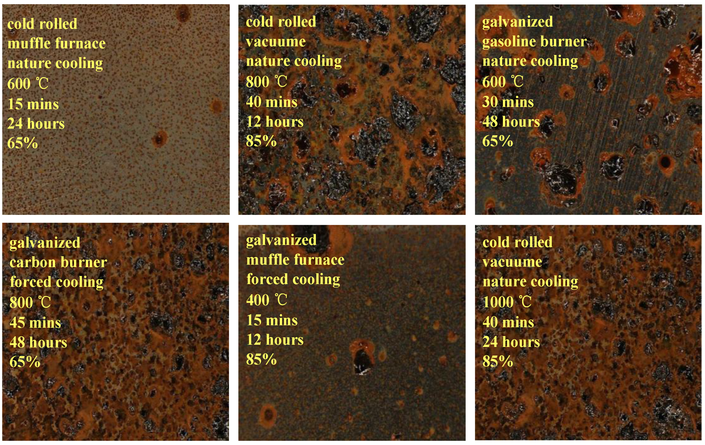
In our previous work, 900 sample images were generated and labeled. We used the same method to create image samples in this work. Galvanized steel and cold rolled steel were selected as basic research objects. The metal plate was cut to equal size (1.0 cm × 1.0 cm × 1.0 mm). According to requirements in Table 2, four devices, vacuum resistance furnace, muffle furnace, gasoline burner and carbon furnace, were used for simulating four heating scenes. After heating with a specific temperature $\left(a_3\right)$ and duration time $\left(a_4\right)$, metals were placed in a test chamber with constant temperature and humidity. Thus, attributes $a_5$, $a_6$ and $a_7$ were employed. Special-purpose microscope was used to screen heated metal mark image samples. All devices used were the same as our previous work. Thus, the figure demonstrations are omitted here. The image sample was captured with a resolution of $2152\times 1616$ pixels, each was labeled with seven attribute values as described in Table 2. Thus, 900 new image samples were generated, and Figure 1 gives some demonstrations.

4. Methodology

In our study, deep learning models were deployed on mobile or embedded products. Its importance lies in the facts that: (1) It is practical for expert to investigate using mobile intelligent equipment in the fire scene instead of using bulky server in the lab. Doing investigation off-site is not a bad choice. Wee want recognize attribute of heated metal mark without destroying the fire scene as far as possible. The mark of heated metal may change if we take it back to the lab. (2) Many applications are usually very sensitive to the response time of the program, even a small delay in service response has a significant impact for users. As more and more applications are provided with core functions by deep learning models, low latency inference becomes increasingly, important whether we deploy models on cloud or on mobile side.

One way to solve this problem is committed to performing model inference on high-performance cloud servers and transferring model inputs and outputs between clients and servers. However, this solution poses many problems, such as high computing costs, massive data migration over mobile networks, user privacy and increased latency. Model compression technology adopts an alternative way for these scenarios, which requires fewer resources to perform inference. This was the focus of our research. Key technologies, top compressed CNNs models and a proposed multi-label classification method are described in this section.

4.1. Technologies for Model Compression

4.1.1. Weight Pruning

Network weight pruning-based methods explore the redundancy in model parameters and try to remove noncritical ones. Weight pruning curtails redundant parameters completely from neural networks so that one can even skip computations for pruned weights.

Srinivas and Babu [26] explored the data-free pruning method. Han et al. [27] proposed a method to reduce the total parameters and operations. In Ref. [28], all convolutional filters are ranked with $l_1$-norm regularization at each pruning iteration, and m filters with minimum value are deleted. Anwar et al. [29] adopted N Particle Filters for N convolutional layers. Each convolutional unit is set with a value according to its accuracy on a small validation dataset, and the lower one is removed. Pruning is considered as a combinational optimization problem in Ref. [30]. In Ref. [31], each sparse convolutional layer can be performed with a few convolution kernels followed by a sparse matrix multiplication. Lebedev and Lempitsky [32] imposed group sparsity constraints on convolutional filters to prune entries of the convolution kernels in a group-wise fashion. In Ref. [33], a group-sparse regularizer on neurons is introduced during training stage to learn compact CNNs with reduced filters. The method in Ref. [34] adds a structured sparsity regularizer on each layer to reduce trivial filters, channels, or even layers. In filter-level pruning, all of the aforementioned works use $l_{2,1}$-norm regularizers.

4.1.2. Quantization and Sharing

Network weight quantization compresses the model by reducing the number of bits required to represent each weight. It generally divides continuous variation data into discrete values and assigns each specific datum to a fixed value. For example, if a weight is represented with a 32-bit floating-point number and we want to indicate a weight with 100 quantified values, then 7-bit representation is sufficient.

$$argmi{n}_C\sum _{i=1}^k\sum _{w\in c_i}{|w-c_i|}^2$$

(2)

Generally, K-means clustering is a simple and convenient solution to solve the problem of quantization of CNNs weights [35], which is shown in Equation (2). C = {$c_1$,$c_2$,…,$c_k$} denotes the cluster centers we want to compute, and w means original weight. The objective function is to minimize the squared error between all weight and center it belongs to. As a result, each w is quantized to one cluster center. If the number of cluster centers is set with k, then $lo{g}_2\left(k\right)$ bits are used to represent the weight value. Vanhoucke et al. [36,37] proposed 8-bit quantization and 16-bit fixed-point representation. They brought significant speedup, reduce memory usage and decrease loss in accuracy. There were also many methods that directly train CNNs with binary weights, e.g., Binary-Connect [38], BinaryNet [39], and XNORNetworks [40]. The main idea was to learn binary weights or activations during the model training directly. The method in Ref. [41] reduced the precision of weights to ternary values. A HashedNets model was proposed, in which the low cost hash function is used to group weights into hash buckets for sharing [42]. In Ref. [43], a simple regularization method based on soft weight-sharing was proposed.

4.1.3. Matrix Factorization

To reduce the time complexity, tensor factorization is a commonly used method. It is usually based on low rank approximation theory, and a high-dimension tensor can be approximated by multiple one-dimensional tensor products.

Lebedev et al. [44] proposed a canonical polyadic (CP)-decomposition based method that decomposing one network layer into five layers with low complexity. The optimal solution was hard to compute with Stochastic gradient descent (SGD) weight fine-tuning. Denton et al. [45] exploited redundancy of convolutional layer and a tensor decomposition method was devised. It treated two-dimensional tensor decomposition as singular decomposition, and three-dimensional tensor decomposition as two-dimensional decomposition.

Zhang et al. [46] used Singular Value Decomposition (SVD) decomposition for parameter matrix, and proposed a nonlinear optimization method with non-SGD. The cumulative reconstruction error of previous layer is considered in asymmetric reconstruction. Jaderberg et al. [47] used rank 1 convolutional filter to generate M independent basic feature map, and then K × K convolutional filters can be decomposed into 1 × K and K × 1 filters. The output is linearly reconstructed with learned weights. Tai et al. [48] proposed a method for training low rank constraint network. A global optimizer is used for matrix factorization and the redundancy of convolutional filter can be reduced.

Kim et al. [49] proposed a model with one or more tensor trained layer. Tensor is trained for tensor compressing and its filters are generated based on SVD approximation. According to redundancy inside and among channels, sparse decomposition was conducted on channels [31]. Convolutional operation with high cost can be transformed into matrix multiplication. The matrix is then sparsified with regularization term.

Among these model compression methods, matrix factorization based methods are most widely used. Many top compressed CNNs models focus on this, which is illustrated in the next subsection.

4.2. Top Compressed CNNs Models

In this subsection, some state-of-the-art compressed CNNs models used in our study are introduced.

4.2.1. MobileNet

$MobileNets$ was first designed for mobile and embedded vision applications. It was built primarily from depthwise separable convolutional operations [50]. It factorizes a standard convolution into a depthwise convolution and a pointwise convolution. $MobileNets$ applies a single filter to each input channel, and then pointwise convolution combines the outputs with linear combination.

A standard convolution operation has the following computational cost:

$$D_K\times D_K\times M\times N\times D_F\times D_F$$

(3)

where M and N are number of input and output channels, $D_K\times D_K$ is the size of filters, and $D_F\times D_F$ represents the size of feature map. $MobileNets$ splits this into two separate operations, one for filtering and one for combining. Batch normalization and ReLU nonlinearity are used in each layer. The depthwise convolution operation has the following computational cost:

$$D_K\times D_K\times M\times D_F\times D_F$$

(4)

A linear combination of the output of depthwise convolution via $1\times 1$ convolution is needed to generate new features. Thus, the total computation cost of depthwise separable convolution is as follows:

$$D_K\times D_K\times M\times D_F\times D_F+M\times N\times D_F\times D_F$$

(5)

The ratio of computational cost decrease can be shown as follows:

$$\frac{D_K\times D_K\times M\times D_F\times D_F+M\times N\times D_F\times D_F}{D_K\times D_K\times M\times N\times D_F\times D_F}=\frac{1}{N}+\frac{1}{D_K^2}$$

(6)

Moreover, to make the model smaller and faster, two hyper-parameters are proposed, width multiplier $\alpha$ and resolution multiplier $\rho$, which represent the ratio of reduced channels and the size of reduced feature maps, respectively. Finally, The computational cost of depthwise convolution operation with parameters $\alpha$ and $\rho$ can be further expressed as follows:

$$D_K\times D_K\times \alpha M\times \rho D_F\times \rho D_F+\alpha M\times \alpha N\times \rho D_F\times \rho D_F$$

(7)

$MobileNet$ V2 was proposed for further improvement. It was constructed with inverted residuals and linear bottlenecks techniques, which can reduce number of parameters and the loss in activation operation. Combined with single shot detector lite (SSDLite) for object detection, $MobileNet$ V2 is reported to be $35\%$ faster than $MobileNet$ V1, and have 20× less computation and 10× fewer parameters than $YOLO$ V2.

4.2.2. SqueezeNet

$SqueezeNet$ was proposed for preserving accuracy with few parameters [51]. A novel building block, $Firemodule$, is used as the core structure in $SqueezeNet$.

Three main strategies are adopted to construct the $Firemodule$. First, 3 × 3 filters are replaced with 1 × 1 filters. This can make the number of parameters 9× smaller than before. Second, the number of input channels to filters is decreased. The number of parameters in one standard layer can be represented as $N_{channel}\times N_{filter}\times S_{filter}$, where $N_{channel}$ is the number of input channels, $N_{filter}$ is the number of filters and $S_{filter}$ is the size of filter. $Squeeze$ layer is proposed to reduce $N_{filter}$ so the total number of parameters can be further decreased. Third, the network is late downsampled. Usually, layers have small activation feature maps if their stride is larger than 1, and larger activation feature maps can lead to higher performance.

To accomplish the above strategies, $Fire$ module was designed, which consists of a squeeze layer and an expand layer. Squeeze layer has only 1 × 1 convolution filters (Strategy 1) and expand layer has 1 × 1 and 3 × 3 convolution filters. Then, three hyperparameters are set: $s_{1\times 1}$, $e_{1\times 1}$ and $e_{3\times 3}$, which represent the numbers of 1 × 1 convolution filters in squeeze layer, 1 × 1 convolution filters and 3 × 3 convolution filters in expand layer, respectively. $s_{1\times 1}$ is set to be less than ($e_{1\times 1}+e_{3\times 3}$), so the squeeze layer can help to limit the number of input channels to expand layer (Strategy 2). The $SqueezeNet$ model is constructed by stacking many Fire modules. The number of filters per $Fire$ module is increased gradually, and a max-pooling with stride 2 is performed with a certain interval (Strategy 3).

The evaluation demonstrates that the $SqueezeNet$ architecture has 50× fewer parameters than original $AlexNet$ and maintains $AlexNet$-level accuracy on ImageNet. Based on $SqueezeNet$, some works implement it on field programmable gate array (FPGA), and the model parameters can be stored entirely within FPGA and there is no need to access off-chip storage.

4.2.3. ShuffleNet

$ShuffleNet$ was proposed by Zhang et al. [52]. In this method, pointwise group convolutions are first used to reduce the costly dense 1 × 1 convolution computation. Then, a novel channel shuffle operation is designed to overcome the side effects of group convolution, which can help information flow across different feature channels.

Group convolution is an effective way to significantly reduce computation cost. However, the outputs are only derived from certain input channels. This blocks the feature exchange among channel groups and the optimal representation cannot be obtained. We proposed a channel shuffle operation to construct association between input and output channels comprising a convolutional layer with g groups and its output with g × n channels. The dimension of the output is reshaped into (g, n) and it is transposed and flattened as the input of next layer.

A $ShuffleNet$ unit is formed with a 1 × 1 pointwise group convolution layer and follows channel shuffle operation layer. $ShuffleNet$ architecture is mainly built by a stack of $ShuffleNet$ units. This structure has less computational cost in the same condition. Let the input be $c\times h\times w$ with bottleneck channels m, $hw(2\mathrm{cm}+9{\mathrm{m}}^2)$ floating-point operations per seconds (FLOPs) and $hw(2\mathrm{cm}+9{\mathrm{m}}^2/\mathrm{g})$ FLOPs is needed for $ResNet$, while only $hw(2\mathrm{cm}/\mathrm{g}+9\mathrm{m})$ FLOPs is needed for $ShuffleNet$.

It is reported that, compared with the $MobileNet$ architecture, $ShuffleNet$ model obtains superior performance of absolute 7.8% increase in ImageNet Top-1 error with cost of about 40 millions floating-point operations per seconds (MFLOPs). The speedup on hardware has also been tested. With comparable performance, the $ShuffleNet$ achieves 13× speedup over $AlexNet$ on an off-the-shelf ARM-based core device.

In the latest version, $channelsplit$ operation is proposed in $ShuffleNet$ V2. The input of feature channels are first split into two branch channels, respectively. One branch remains the same, and the other branch is computed with 1 × 1 convolution, 3 × 3 depthwise separable convolution and 1 × 1 convolution. Then, the two branch features are concatenated and a channel Shuffle operation is implemented. After the channel shuffle, it is repeated for the next unit.

The report demonstrates that $ShuffleNet$ V2 is about 40% faster than $ShuffleNet$ V1 and about 16% faster than $MobileNet$ V2. With 500 MFLOPs, $ShuffleNet$ V2 is 58% faster than $MobileNet$ V2 and 63% faster than $ShuffleNet$ V1.

4.3. Multi-Label Classification

For an input heated metal mark image, we aimed to recognize its attributes of metal type, heating mode, heating temperature, heating duration, cooling mode, placing duration and relative humidity. Each attribute can be trained with a model, with totally seven separate models. However, this has low efficiency for computation time and storage space even using compressed models. In this study, a multiple label classification method was adopted. Seven attributes were recognized in a single test with one unified CNNs model.

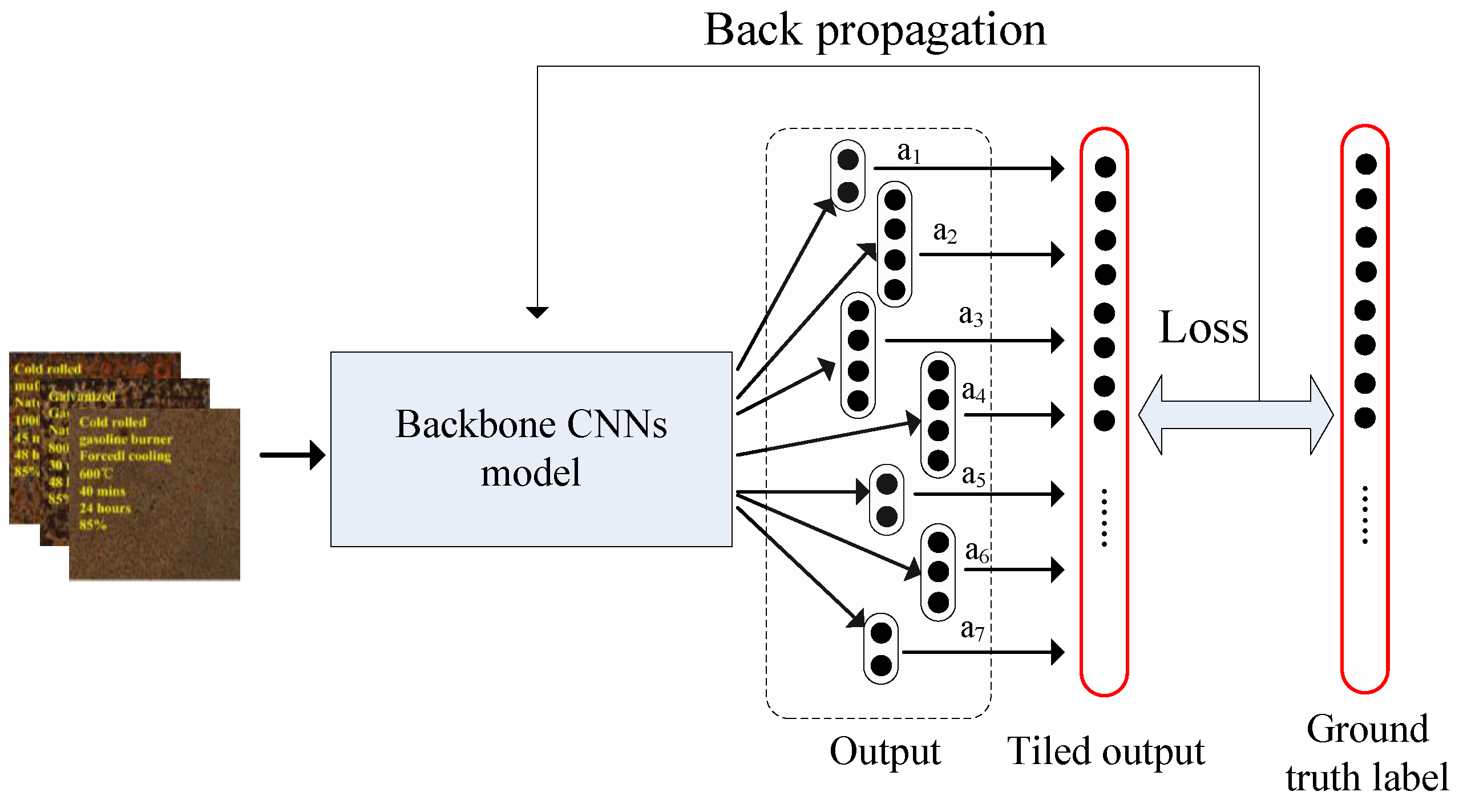
Figure 2 gives the basic procedure. For each attribute $a_i$, its type was represented with one-hot encoding mode. Then, two-dimensional feature vector, four-dimensional feature vector, four-dimensional feature vector, four-dimensional feature vector, two-dimensional feature vector, three-dimensional feature vector and two-dimensional feature vector were encoded for attributes $a_1$–$a_7$, respectively. All attributes shared the same backbone network model. All outputs were formed into a tiled vector, and the ground truth labels were concatenated into the same pattern. Finally, the objective function was formulated as follows.

$$\begin{array}{cc}\hfill J\left(\theta \right)& =argmi{n}_{\theta }\sum _{i=1}^{n}L(f(x^i;\theta ),y^i)\hfill \\ & =argmi{n}_{\theta }\sum _{i=1}^n\sum _{j=1}^7{w}_j\times L(f(x^i;{\theta }_j),y_j^i)\hfill \end{array}$$

(8)

As shown in Equation (8), $\{x^i,y^i\}$ represents training image sample. Total loss was composed of seven sub-loss, each corresponding to an attribute. $\theta =\{{\theta }_1,{\theta }_2,{\theta }_3,{\theta }_4,{\theta }_5,{\theta }_6,{\theta }_7\}$, $y^i=\{y_1^i,y_2^i,y_3^i,y_4^i,y_5^i,y_6^i,y_7^i\}$, $w_i$ is weight parameter and $cross$-$entropy$ is adopted for $L\left(\right)$.

5. Experimental Evaluation

5.1. Experiment Setup

The performances of heated metal mark attributes recognition with compressed CNNs models were evaluated based on a generated benchmark dataset. In this experiment, Python was used as programming language. Tensorflow was adopted as deep learning framework and Keras was selected as library. All experiments were evaluated on Pentium I5-8 series CPU, 32G RAM, Nvidia GTX TitanXp 12G GPU, Ubuntu OS PC.

5.2. Recognition Accuracy Evaluation

Recognition accuracy was used to evaluate recognition performance on different attribute. As shown in Equation (9), $R_i$ is the recognition accuracy for attribute $a_i$, $N_i^{all}$ means the number of all testing samples containing $a_i$, and $N_i^{correct}$ denotes the number of correctly recognized attribute $a_i$. We divided the dataset into six subgroups with attribute values equally distributed. Five randomly chosen subgroups (1500 image samples) were used for training and the remaining subgroup (300 image samples) was used for testing. The results were obtained by averaging the five independent tests.

$$R_i=\frac{N_i^{correct}}{N_i^{all}}$$

(9)

$MobileNet$, $ShuffleNet$ and $SqueezeNet$ were used as backbone compressed CNNs models for evaluation. For model input, sample image size was set as 224 × 224 × 3 pixels. Epoch was set as 50 and batch size was set as 32. Adam was used as preferred optimization method. Learning rate was set with initial value of 0.001 and momentum was set as 0.9. Dropout was set as 0.2.

The results of average recognition accuracy are shown in

Table 3. Recognition accuracy for seven attributes.

CNNs Model	Data Augment	${\mathit{a}}_1$	${\mathit{a}}_2$	${\mathit{a}}_3$	${\mathit{a}}_4$	${\mathit{a}}_5$	${\mathit{a}}_6$	${\mathit{a}}_7$	$\mathit{overall}$
$MobileNet$	yes	0.785	0.829	0.778	0.786	0.883	0.817	0.885	0.822
	no	0.732	0.816	0.765	0.745	0.871	0.809	0.868	0.801
$ShuffleNet$	yes	0.803	0.809	0.804	0.812	0.878	0.813	0.894	0.830
	no	0.731	0.798	0.789	0.810	0.848	0.805	0.865	0.807
$SqueezeNet$	yes	0.68	0.837	0.825	0.774	0.858	0.758	0.887	0.803
	no	0.657	0.829	0.814	0.752	0.849	0.674	0.862	0.777

. Structure of CNNs models and data augment are listed in the first and second columns, respectively. For data augment, commonly used transformations including random cropping, vertical and horizontal flipping, perturbation of brightness, saturation, hue and contrast were adopted. When the model was trained with data augment, $40\%$ of training image in each batch was augmented, otherwise the probability was $10\%$. For $a_1$, $ShuffleNet$ with data augment obtained the best performance, with value of 0.803. For $a_2$, $SqueezeNet$ with data augment obtained best performance, with value of 0.837. For $a_3$, $SqueezeNet$ with data augment obtained best performance, with value of 0.825. For $a_4$, $ShuffleNet$ with data augment obtained best performance, with value of 0.812. For $a_5$, $MobileNet$ with data augment obtained best performance, with value of 0.883. For $a_6$, $MobileNet$ and $ShuffleNet$ with data augment obtained best performance, with value of 0.817. For $a_7$, $ShuffleNet$ with data augment obtained best performance, with value of 0.894. For the overall performances, $ShuffleNet$ model ranked first.

We found that models training with data augment obtained better performance than those without data augment. There was about 2% accuracy improvement. It can be concluded that data augment is an effective way to train better CNN models, especially for large scale CNNs with huge parameters and lacking of sufficient training data.

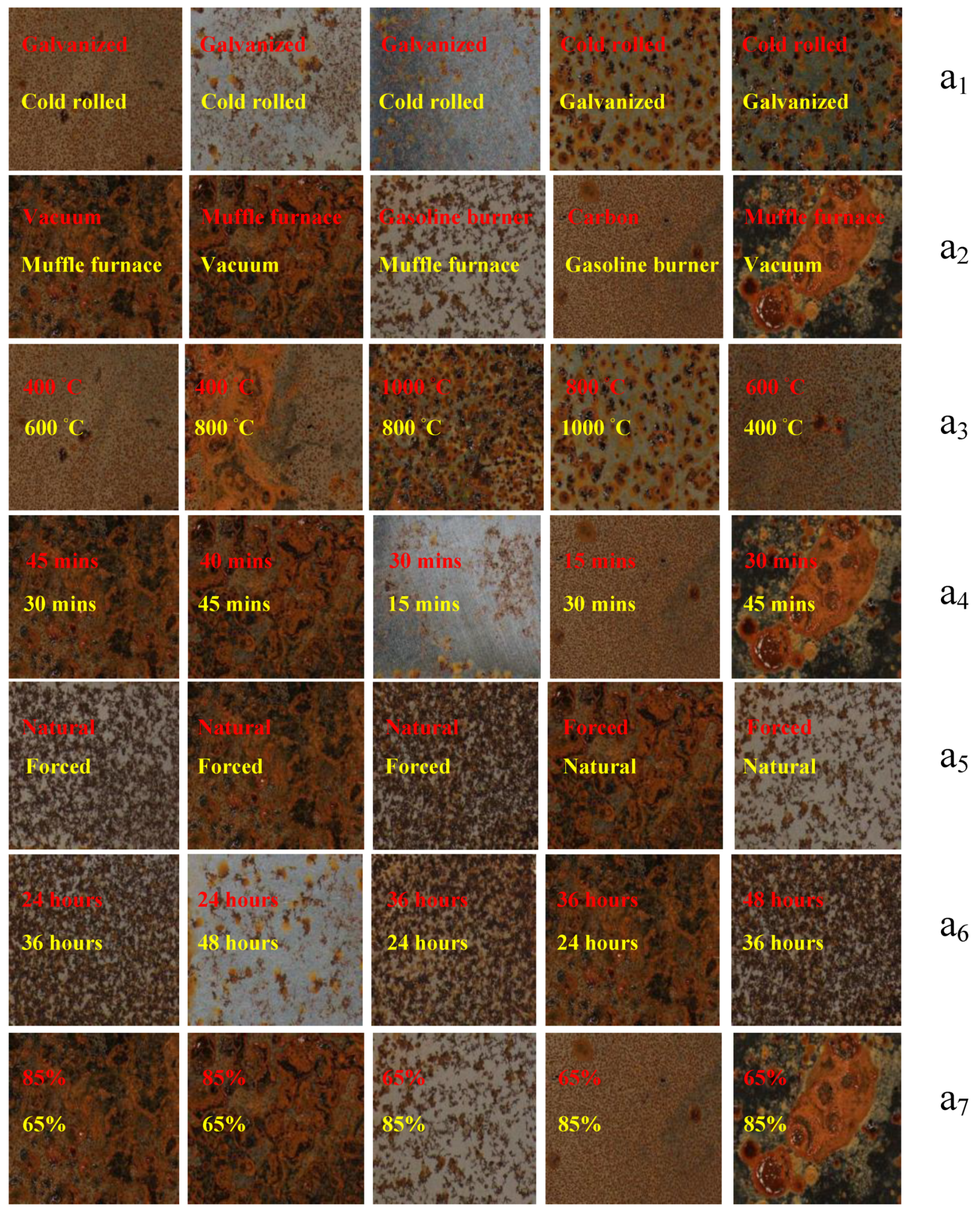
Figure 3 demonstrates the misclassified sample images. Each row corresponds to an attribute. The red texts represent ground truth label, while yellow texts represent the predicted results. Galvanized steel and cold rolled steel normally have different corrosion degrees at the experimental condition. The misclassified sample images of $a_1$ showed similar corrosion degree. For heating temperature, higher temperatures will lead to more corrosion and rougher texture. The misclassified sample images of $a_3$ came from adjacent temperature. These situations can be seen as general causes of $a_4$, $a_6$ and $a_7$. For $a_2$ and $a_5$, the reason for misclassification is hard to describe even for the field professional.

Commonly used large scale datasets are mainly natural scene, animals, etc. These are easy to distinguish by humans, and the differences are easy to explain visually. The heated metal mark image we studied is a special kind of objects, the origin of its mark being caused by complex physical and chemical reactions. Moreover, the benchmark dataset we generated inevitably contains noise, which may influence the model performance. We need further research to explore the internal principle with the help of other professionals.

5.3. Batch Size Evaluation

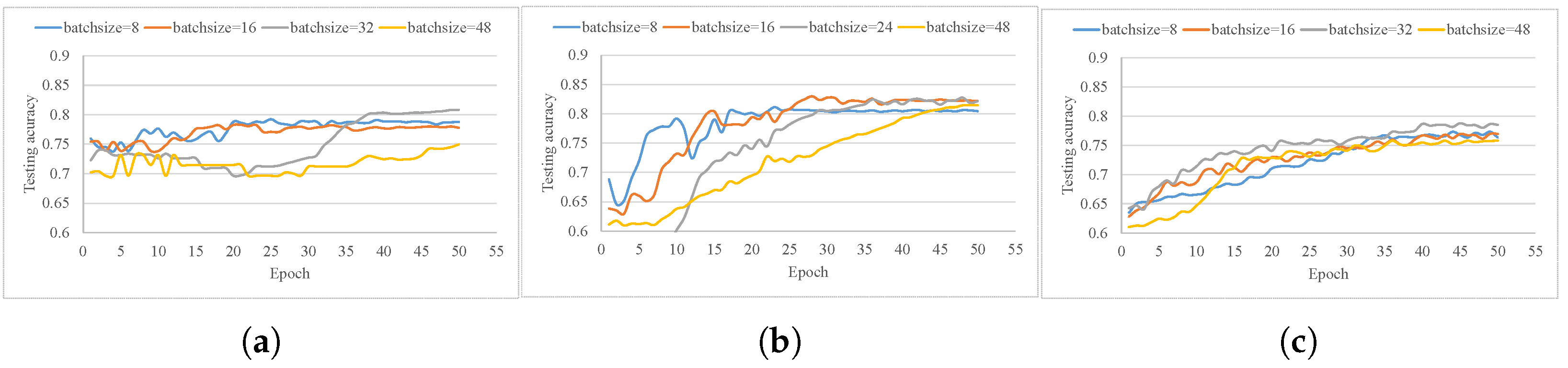
Training on different batch sizes, 8, 16, 32 and 48 was evaluated. Figure 4 demonstrates the model accuracy versus training epoch. Here, the average accuracy over seven attribute was used. Data augment was used and other parameters were set the same as for the experiments presented in Section 5.2.

As shown in the figure, all models converged after about 40 training epochs. Models trained with batchsize 32 obtained better performance, and outperformed other models by about $2\%$. $SqueezeNet$ was more stable and smooth during training, while $MobileNet$ and $ShuffleNet$ fluctuated more. It was reasonably found that for bigger batch sizes the gradient descent direction computation was more accurate, and was gentler during model training. Smaller batch sizes led to more randomness, and it was harder to achieve optimal performance.

5.4. Single Label Model vs. Multi-Label Model

The plain way to train models is to train an independent CNN model for each attribute. This is called single label model. Comparisons between single label model and multi-label model were evaluated. Single label model was trained separately for each attribute $a_i$. The results are shown in

Table 4. Single label model vs. multi-label model.

CNNs Model	Single/Multi Label	${\mathit{a}}_1$	${\mathit{a}}_2$	${\mathit{a}}_3$	${\mathit{a}}_4$	${\mathit{a}}_5$	${\mathit{a}}_6$	${\mathit{a}}_7$	$\mathit{overall}$
$MobileNet$	multi	0.785	0.829	0.778	0.786	0.883	0.817	0.885	0.822
	single	0.815	0.847	0.807	0.805	0.899	0.819	0.894	0.841
$ShuffleNet$	multi	0.803	0.809	0.804	0.812	0.878	0.813	0.894	0.830
	single	0.824	0.829	0.811	0.824	0.870	0.824	0.912	0.842
$SqueezeNet$	multi	0.68	0.837	0.825	0.774	0.858	0.758	0.887	0.803
	single	0.767	0.842	0.831	0.792	0.877	0.764	0.891	0.823

.

It can be seen from the result that models with single label training obtained better performance than those with multi-label training, with about 1–$2\%$ improvement. There were some divergences for different attributes, but the overall trends were consistent.

Using multi-label training, model parameters could be shared. The size of model was greatly reduced by 7×, with some performance loss. Multi-label training is not a trivial task as there are conflicts among training parameters for recognizing different attribute. The loss scale for different attribute may be very large, thus the model training could not be coherent for seven attributes. Therefore, the learning process of shared parameters was unavoidably influenced.

5.5. Compressed Model vs. Heavy Model

Different CNN models contain various depth and width of layers, number of filters, size and shape of filters, which lead to different structures, parameters and complexity. Comparisons between compressed models and heavy models were evaluated. $VGG16$, $ResNet50$, and $Inception$ models were selected. The results are shown in

Table 5. Compressed model vs. heavy model.

CNNs Model	${\mathit{a}}_1$	${\mathit{a}}_2$	${\mathit{a}}_3$	${\mathit{a}}_4$	${\mathit{a}}_5$	${\mathit{a}}_6$	${\mathit{a}}_7$	$\mathit{overall}$
$MobileNet$	0.785	0.829	0.778	0.786	0.883	0.817	0.885	0.822
$ShuffleNet$	0.803	0.809	0.804	0.812	0.878	0.813	0.894	0.830
$SqueezeNet$	0.68	0.837	0.825	0.774	0.858	0.758	0.887	0.803
$VGG16$	0.810	0.845	0.840	0.817	0.892	0.821	0.899	0.846
$ResNet50$	0.819	0.851	0.835	0.826	0.881	0.829	0.905	0.849
$Inception$	0.821	0.852	0.841	0.832	0.901	0.831	0.909	0.854

.

It can be seen that heavy CNNs models obtained better performance for all attribute than compressed models. $Inception$ obtained an average performance of 0.854, which was $2.4\%$ better than $ShuffleNet$. The main reason is that heavy models contain more complex structures and more parameters, which have the advantages of feature extraction and representation. However, the performance differences between compressed models and heavy models were not large, at only about 1–$2\%$.

5.6. Running Time Evaluation

Running time of different CNN models was evaluated. Training and testing time of $MobileNet$, $SqueezeNet$, $ShuffleNet$ and $ResNet50$ models with various batch sizes (8, 16, 32 and 48) were evaluated.

Table 6. Execution time (seconds).

Execution Time	Batch Size	$\mathit{MobileNet}$	$\mathit{SqueezeNet}$	$\mathit{ShuffleNet}$	$\mathit{ResNet}50$
Training time	8	0.192	0.024	0.08	0.438
	16	0.368	0.032	0.144	0.889
	32	0.736	0.064	0.256	1.554
	48	1.104	0.144	0.384	2.862
Testing time	x	0.0095	0.0026	0.0065	0.031
Space occupation	x	9.6M	3.1M	5M	94.7M

gives the experiment results.

$MobileNet$ cost the longest training time among all three compressed CNNs models, at 0.192 s, 0.368 s, 0.736 s and 1.104 s for batch sizes of 8, 16, 32 and 48, respectively, during each training iteration. $SqueezeNet$ used the shortest training time, with about $80\%$ of $MobileNet$’s. For testing time, $SqueezeNet$ had the minimal cost, 0.0026 s. Comparing with $ResNet50$ model, the running efficiency was greatly improved with compressed CNNs models. All execution times were evaluated on PC. For model space occupancy, 9.6 M, 3.1 M and 5 M were required for $MobileNet$, $SqueezeNet$ and $ShuffleNet$, while 94.7 M was needed for $ResNet50$. This also demonstrated the space efficiency of compressed CNN models. $SqueezeNet$ model rand 10× faster than $ResNet50$ model, and reduced the storage space by 30×.

5.7. Android Devices Deployment

The models were trained on a PC Server. They were properly running on Linux with Tensorflow framework. However, this could not be done directly on a mobile devices, and some essential transformation and deployment were needed. The compressed CNNs models were deployed on Android platforms, and the corresponding performances were also tested.

The file format of CNNs model on Linux was *.h5. It was first converted into format of *.pb to deploy on Android devices. The file size of $MobileNet$, $SqueezeNet$ and $ShuffleNet$ models were 2.82 MB, 4.02 MB and 9.06 MB, respectively, after format conversion, which were similar to their PC format.

Table 7. Execution time on Android devices (seconds).

CNNs Models	Snapdragon 626	Snapdragon 845	Kylin 970	Our PC Server
$\mathit{MobileNet}$	0.055	0.021	0.014	0.0095
$\mathit{SqueezeNet}$	0.018	0.011	0.0076	0.0026
$\mathit{ShuffleNet}$	0.039	0.015	0.0108	0.0065

gives the result of model testing on selected Android platforms. $Snapdragon$ 626, $Snapdragon$ 845 and $Kylin$ 970 were used for testing. As can be seen form the result, mobile devices showed good efficiency, and could execute the operation in tens of milliseconds, thus could support real-time applications. $Kylin$ 970 obtained the best performance, and it cost 0.00076 s to execute the $SqueezeNet$ model. This might derive from the Neural Network Processing Unit it contains.

6. Conclusions

Heated metal marks are important evidence for fire scene analysis. Automatic heated metal attribute recognition using deep learning method has become popular. To further improve the model efficiency, this study considered heated metal mark image attribute recognition based on compressed CNNs model. We expanded the benchmark dataset. Three well known compressed CNNs models were used as backbone structure and a multi-label training method was adopted. Comprehensive experiment were evaluated and analyzed, including recognition rate, influence of batchsize, compressed model vs. heavy model, single label model vs. multi-label model, etc. Moreover, compressed CNNs models were deployed and tested on Android devices.

Through this study, it can be concluded that using compressed CNNs model, efficiency of both time and space are greatly improved, and recognition accuracy still lies in acceptable range. According to the experiment evaluation, $ShuffleNet$ has the best over recognition accuracy, and $SqueezeNet$ costs the minimal running time. Therefore, users can adopt any models based on their actual demands.

References

- Inspection Methods for Trace and Physical Evidences from Fire Scene—Part 3: Ferrous Metal Work; GB/T 27905.3-2011; National Standard of People’s Republic of China: Shenzhen, China, 2011.
- Wu, Y.; Zhao, C.; Di, M.; Qi, Z. Application of metal oxidation theory in fire trace evidence identification. In Proceedings of the Building Electrical and Intelligent System, Shenyang, China, 11–13 November 2007; pp. 108–110. [Google Scholar]
- Wu, Y.; Zhao, C.; Di, M.; Qi, Z. Application of metal oxidation theory in fire investigation and fire safety. In Proceedings of the International Colloquium on Safety Science and Technology, Shenyang, China, 27–28 October 2008; pp. 538–540. [Google Scholar]
- Xu, Z.; Song, Y. Fuzzy identification of surface temperature for building members after fire. J. Dalian Univ. Technol. 2005, 45, 853–857. [Google Scholar]
- Lowe, D.G. Object Recognition from Local Scale-Invariant Features. In Proceedings of the IEEE International Conference on Computer Vision, Kerkyra, Greece, 20–27 September 1999; pp. 1150–1157. [Google Scholar]
- Lowe, D.G. Distinctive Image Features from Scale-Invariant Keypoints. Int. J. Comput. Vis. 2006, 60, 91–110. [Google Scholar] [CrossRef]
- Navneet, D.; Bill, T. Histograms of Oriented Gradients for Human Detection. In Proceedings of the IEEE Computer Society Conference on Computer Vision and Pattern Recognition, San Diego, CA, USA, 20–25 June 2005; pp. 886–893. [Google Scholar]
- Bay, H.; Tuytelaars, T.; van Gool, L. SURF: Speeded Up Robust Features. In Proceedings of the 9th European Conference on Computer Vision, Graz, Austria, 7–13 May 2006; pp. 404–417. [Google Scholar]
- Wang, X.; Han, T.X.; Yan, S. An HOG-LBP human detector with partial occlusion handling. In Proceedings of the IEEE 12th International Conference on Computer Vision, Kyoto, Japan, 27 September–4 October 2009; pp. 32–39. [Google Scholar]
- Fei-Fei, L.; Fergus, R.; Torralba, A. Recognizing and Learning Object Categories. CVPR 2007 Short Course. Available online: http://people.csail.mit.edu/torralba/shortCourseRLOC/ (accessed on 18 March 2018).
- Grauman, K.; Darrell, T. The Pyramid Match Kernel: Discriminative Classification with Sets of Image Features. In Proceedings of the 10th IEEE International Conference on Computer Vision, Beijing, China, 17–21 October 2005; pp. 1458–1465. [Google Scholar]
- LeCun, Y.; Boser, B.; Denker, J.S.; Henderson, D.; Howard, R.E.; Hubbard, W.; Jackel, L.D. Backpropagation Applied to Handwritten Zip Code Recognition. Neural Comput. 1989, 1, 541–551. [Google Scholar] [CrossRef]
- LeCun, Y.; Bottou, L.; Bengio, Y.; Haffner, P. Gradient Based Learning Applied to Document Recognition. Proc. IEEE 1998, 86, 2278–2324. [Google Scholar] [CrossRef]
- Krizhevsky, A.; Sutskever, I.; Hinton, G.E. ImageNet Classification with Deep Convolutional Neural Networks. In Proceedings of the 26th Annual Conference on Neural Information Processing Systems, Lake Tahoe, NE, USA, 3–6 December 2012; pp. 1106–1114. [Google Scholar]
- Zeiler, M.D.; Fergus, R. Visualizing and Understanding Convolutional Networks. In Proceedings of the 13th European Conference on Computer Vision, Zurich, Switzerland, 6–12 September 2014; pp. 818–833. [Google Scholar]
- Simonyan, K.; Zisserman, A. Very Deep Convolutional Networks for Large-Scale Image Recognition. In Proceedings of the International Conference on Learning Representations, San Diego, CA, USA, 7–9 May 2015; pp. 1–14. [Google Scholar]
- Szegedy, C.; Liu, W.; Jia, Y.; Sermanet, P.; Reed, S.; Anguelov, D.; Erhan, D.; Vanhoucke, V.; Rabinovich, A. Going deeper with convolutions. In Proceedings of the IEEE Conference on Computer Vision and Pattern Recognition, Boston, MA, USA, 7–12 June 2015; pp. 1–9. [Google Scholar]
- He, K.; Zhang, X.; Ren, S.; Sun, J. Deep Residual Learning for Image Recognition. In Proceedings of the IEEE Conference on Computer Vision and Pattern Recognition, Las Vegas, NV, USA, 27–30 June 2016; pp. 770–778. [Google Scholar]
- Faghih-Roohi, S.; Hajizadeh, S.; Núñez, A.; Babuska, R.; De Schutter, B. Deep convolutional neural networks for detection of rail surface defects. In Proceedings of the International Joint Conference on Neural Networks, Vancouver, BC, Canada, 24–29 July 22016; pp. 2584–2589. [Google Scholar]
- Li, S.; Liu, G.; Tang, X.; Lu, J.; Hu, J. An Ensemble Deep Convolutional Neural Network Model with Improved D-S Evidence Fusion for Bearing Fault Diagnosis. Sensors 2017, 17, 1729. [Google Scholar] [CrossRef] [PubMed]
- Psuj, G. Multi-Sensor Data Integration Using Deep Learning for Characterization of Defects in Steel Elements. Sensors 2018, 18, 292. [Google Scholar] [CrossRef] [PubMed]
- Zhou, S.; Chen, Y.; Zhang, D.; Xie, J.; Zhou, Y. Classification of surface defects on steel sheet using convolutional neural networks. Mater. Technol. 2017, 51, 123–131. [Google Scholar] [CrossRef]
- Cha, Y.J.; Choi, W.; Büyüköztürk, O. Deep Learning-Based Crack Damage Detection Using Convolutional Neural Networks. Comput.-Aided Civ. Infrastruct. Eng. 2018, 32, 361–378. [Google Scholar] [CrossRef]
- Cha, Y.J.; Choi, W.; Suh, G.; Mahmoudkhani, S.; Büyüköztürk, O. Autonomous Structural Visual Inspection Using Region-Based Deep Learning for Detecting Multiple Damage Types. Comput.-Aided Civ. Infrastruct. Eng. 2017. [Google Scholar] [CrossRef]
- Mao, K.; Lu, D.; E, D.; Tan, Z. A Case Study on Attribute Recognition of Heated Metal Mark Image Using Deep Convolutional Neural Networks. Sensors 2018, 18, 1871. [Google Scholar] [CrossRef] [PubMed]
- Srinivas, S.; Babu, R.V. Data-free parameter pruning for deep neural networks. In Proceedings of the British Machine Vision Conference, Swansea, UK, 7–10 September 2015; p. 31. [Google Scholar]
- Han, S.; Pool, J.; Tran, J.; Dally, W.J. Learning both weights and connections for efficient neural networks. In Proceedings of the 28th International Conference on Neural Information Processing Systems, Montreal, QC, Canada, 7–12 December 2015; pp. 1135–1143. [Google Scholar]
- Li, H.; Kadav, A.; Durdanovic, I.; Samet, H.; Graf, H.P. Pruning filters for effecient convnets. In Proceedings of the International Conference on Learning Representations (ICLR 2017), Toulon, France, 24–26 April 2017. [Google Scholar]
- Anwar, S.; Hwang, K.; Sung, W. Structured Pruning of Deep Convolutional Neural Networks. In Proceedings of the JETC 2017, Budapest, Germany, 21–25 May 2017; Volume 13, p. 32. [Google Scholar]
- Molchanov, P.; Tyree, S.; Karras, T.; Aila, T.; Kautz, J. Pruning Convolutional Neural Networks for Resource Effificient Transfer Learning. In Proceedings of the NIPS Workshop: The 1st International Workshop on Effificient Methods for Deep Neural Networks, Barcelona, Spain, 5–10 June 2016. [Google Scholar]
- Liu, B.; Wang, M.; Foroosh, H.; Tappen, M.F.; Pensky, M. Sparse Convolutional Neural Networks. In Proceedings of the IEEE Conference on Computer Vision and Pattern Recognition (CVPR 2015), Boston, MA, USA, 7–12 June 2015; pp. 806–814. [Google Scholar]
- Lebedev, V.; Lempitsky, V.S. Fast convnets using group-wise brain damage. In Proceedings of the IEEE Conference on Computer Vision Pattern Recognition, Las Vegas, NV, USA, 26 June–1 July 2016; pp. 2554–2564. [Google Scholar]
- Zhou, H.; Alvarez, J.M.; Porikli, F. Less is more: Towards compact CNNs. In Proceedings of the European Conference on Computer Vision, Amsterdam, The Netherlands, 8–16 October 2016; pp. 662–677. [Google Scholar]
- Wen, W.; Wu, C.; Wang, Y.; Chen, Y.; Li, H. Learning structured sparsity in deep neural networks. Adv. Neural Inform. Process. Syst. 2016, 29, 2074–2082. [Google Scholar]
- Wu, J.; Leng, C.; Wang, Y.; Hu, Q.; Cheng, J. Quantized convolutional neural networks for mobile devices. In Proceedings of the IEEE Conference on Computer Vision Pattern Recognition, Las Vegas, NV, USA, 26 June–1 July 2016; pp. 4820–4828. [Google Scholar]
- Vanhoucke, V.; Senior, A.; Mao, M.Z. Improving the speed of neural networks on cpus. In Proceedings of the Conference on Neural Information Processing Systems Deep Learning and Unsupervised Feature Learning Workshop, Sierra Nevada, Spain, 16–17 December 2011. [Google Scholar]
- Gupta, S.; Agrawal, A.; Gopalakrishnan, K.; Narayanan, P. Deep learning with limited numerical precision. In Proceedings of the 32nd International Conference on Machine Learning, Lille, France, 6–11 July 2015; Voume 37; pp. 1737–1746. [Google Scholar]
- Courbariaux, M.; Bengio, Y.; David, J. Binaryconnect: Training deep neural networks with binary weights during propagations. In Proceedings of the Annual Conference on Neural Information Processing Systems, Montreal, QC, Canada, 7–12 December 2015; pp. 3123–3131. [Google Scholar]
- Courbariaux, M.; Bengio, Y. Binarynet: Training deep neural networks with weights and activations constrained to +1 or −1. arXiv 2016, arXiv:1602.02830. [Google Scholar]
- Rastegari, M.; Ordonez, V.; Redmon, J.; Farhadi, A. Xnor-net: Imagenet classification using binary convolutional neural networks. In Proceedings of the European Conference on Computer Vision, Amsterdam, The Netherlands, 8–16 October 2016; pp. 525–542. [Google Scholar]
- Zhu, C.; Han, S.; Mao, H.; Dally, W.J. Trained ternary quantization. arXiv 2016, arXiv:1612.01064. [Google Scholar]
- Chen, W.; Wilson, J.; Tyree, S.; Weinberger, K.Q.; Chen, Y. Compressing neural networks with the hashing trick. In Proceedings of the Machine Learning Research Workshop Conference, Montreal, QC, Canada, 12 December 2015; pp. 2285–2294. [Google Scholar]
- Ullrich, K.; Meeds, E.; Welling, M. Soft weight-sharing for neural network compression. arXiv 2017, arXiv:1702.04008. [Google Scholar]
- Lebedev, V.; Ganin, Y.; Rakhuba, M.; Oseledets, I.V.; Lempitsky, V.S. Speeding-up Convolutional Neural Networks Using Fine-tuned CP-Decomposition. arXiv 2014, arXiv:1412.6553. [Google Scholar]
- Denton, E.L.; Zaremba, W.; Bruna, J.; LeCun, Y.; Fergus, R. Exploiting linear structure within convolutional networks for efficient evaluation. In Proceedings of the NIPS 2014, Montreal, QC, Canada, 8–13 December 2014. [Google Scholar]
- Zhang, X.; Zou, J.; He, K.; Sun, J. Accelerating Very Deep Convolutional Networks for Classification and Detection. IEEE Trans. Pattern Anal. Mach. Intell. 2016, 38, 1943–1955. [Google Scholar] [CrossRef] [PubMed]
- Jaderberg, M.; Vedaldi, A.; Zisserman, A. Speeding up Convolutional Neural Networks with Low Rank Expansions. In Proceedings of the BMVC 2014, Nottingham, UK, 1–5 September 2014. [Google Scholar]
- Tai, C.; Xiao, T.; Zhang, Y.; Wang, X.; E, W. Convolutional neural networks with low-rank regularization. In Proceedings of the ICLR 2016, San Juan, Puerto Rico, 2–4 May 2016. [Google Scholar]
- Kim, Yo.; Park, E.; Yoo, S.; Choi, T.; Yang, L.; Shin, D. Compression of Deep Convolutional Neural Networks for Fast and Low Power Mobile Applications. In Proceedings of the ICLR 2016, San Juan, Puerto Rico, 2–4 May 2016. [Google Scholar]
- Howard, A.G.; Zhu, M.; Chen, B.; Kalenichenko, D.; Wang, W.; Weyand, T.; Andreetto, M.; Adam, H. MobileNets: Efficient Convolutional Neural Networks for Mobile Vision Applications. arXiv 2017, arXiv:1704.04861. [Google Scholar]
- Iandola, F.N.; Moskewicz, M.W.; Ashraf, K.; Han, S.; Dally, W.J.; Keutzer, K. SqueezeNet: AlexNet-level accuracy with 50x fewer parameters and <1 MB model size. arXiv 2016, arXiv:1602.07360. [Google Scholar]
- Zhang, X.; Zhou, X.; Lin, M.; Sun, J. ShuffleNet: An Extremely Efficient Convolutional Neural Network for Mobile Devices. arXiv 2017, arXiv:1707.01083. [Google Scholar]
Figure 1.
Demonstration of generated heated metal mark image samples. Seven attributes are labeled on the top-left position of each image.
Figure 2.
Demonstration of multi-label model training.
Figure 3.
Demonstration of error classified samples. Red texts represent ground truth label, while yellow texts represent the predicted results.
Figure 4.
Model accuracy versus training epoch on various batchsize: (a) result on MobileNet model; and (b,c) result on ShuffleNet and SqueezeNet models, respectively. Blue, orange, gray and yellow curves represent batchsizes equal 8, 16, 32 and 48, respectively.