Nondestructive Determination and Visualization of Quality Attributes in Fresh and Dry Chrysanthemum morifolium Using Near-Infrared Hyperspectral Imaging

Abstract

Rapid and nondestructive determination of quality attributes in fresh and dry Chrysanthemum morifolium is of great importance for quality sorting and monitoring during harvest and trade. Near-infrared hyperspectral imaging covering the spectral range of 874–1734 nm was used to detect chlorogenic acid, luteolin-7-O-glucoside, and 3,5-O-dicaffeoylquinic acid content in Chrysanthemum morifolium. Fresh and dry Chrysanthemum morifolium flowers were studied for harvest and trade. Pixelwise spectra were preprocessed by wavelet transform (WT) and area normalization, and calculated as average spectrum. Successive projections algorithm (SPA) was used to select optimal wavelengths. Partial least squares (PLS), extreme learning machine (ELM), and least-squares support vector machine (LS-SVM) were used to build calibration models based on full spectra and optimal wavelengths. Calibration models of fresh and dry flowers obtained good results. Calibration models for chlorogenic acid in fresh flowers obtained best performances, with coefficient of determination (R²) over 0.85 and residual predictive deviation (RPD) over 2.50. Visualization maps of chlorogenic acid, luteolin-7-O-glucoside, and 3,5-O-dicaffeoylquinic acid in single fresh and dry flowers were obtained. The overall results showed that hyperspectral imaging was feasible to determine chlorogenic acid, luteolin-7-O-glucoside, and 3,5-O-dicaffeoylquinic acid. Much more work should be done in the future to improve the prediction performance.

1. Introduction

Flowers used as tea sources have lasted for centuries due to their unique taste and aroma. Chrysanthemum tea is one of the mostly consumed flower teas, with a large family of Chrysanthemum species. Chrysanthemum morifolium (namely Hangbaiju in China) is one of the Chrysanthemum teas with good fame. Chrysanthemum morifolium planted in Tongxiang (Zhejiang Province, China) is one of the China Protected Geographical Indication Products with high commercial value. Despite its unique taste and aroma, Chrysanthemum morifolium also has medical benefit such as antipyretic and sedative effects, reducing blood pressure and reducing eye strain [1].

Chlorogenic acid, luteolin-7-O-glucoside, and 3,5-O-dicaffeoylquinic acid are the main active ingredients in Chrysanthemum morifolium. Medical benefits of these three ingredients have been reported in literature [2,3,4]. Determination of chlorogenic acid, luteolin-7-O-glucoside, and 3,5-O-dicaffeoylquinic acid content is of great importance for quality monitoring of Chrysanthemum morifolium. Traditional methods such as high-performance liquid chromatography (HPLC) listed in the Chinese Pharmacopoeia [5] are used for chlorogenic acid, luteolin-7-O-glucoside, and 3,5-O-dicaffeoylquinic acid measurement. Laboratory-based chemical methods are time-consuming, high cost, reagent-wasteful, and sample-destructive, and these techniques need complex operation skills. Although these methods can obtain accurate measurement results, they cannot be used to measure a large batch of samples in a short time. Thus, rapid, nondestructive, and accurate techniques are needed.

Hyperspectral imaging is one of the rapid and nondestructive techniques. Hyperspectral imaging integrates imaging technique and spectroscopy technique, and it can acquire spatial and spectral information simultaneously. Due to this characteristic, hyperspectral imaging has been used in various fields, such as food [6,7], agriculture [8,9], medicine [10,11], and so forth. Hyperspectral imaging can acquire spectral information of each pixel within the research samples, and hyperspectral images can be analyzed at pixelwise level [12,13].

Generally, dry Chrysanthemum morifolium are stored and consumed in the market. The fresh Chrysanthemum morifolium are harvested, undergo enzyme deactivation, and are dried. Determination of quality attributes of dry Chrysanthemum morifolium is important for Chrysanthemum morifolium trade and consumption. Moreover, it is important to determine quality attributes of fresh Chrysanthemum morifolium during harvest. Knowing quality attributes will help to optimize the harvest time and procedure of Chrysanthemum morifolium, and the quality sorting can be conducted during harvest. Our previous study has proven the feasibility of using hyperspectral imaging to determine total polysaccharides and total flavonoids in dry Chrysanthemum morifolium [14]. The feasibility of using hyperspectral imaging to determine more chemical compositions for quality sorting and monitoring of Chrysanthemum morifolium should be further studied.

The objective of this study was to determine chlorogenic acid, luteolin-7-O-glucoside, and 3,5-O-dicaffeoylquinic acid content in fresh and dry Chrysanthemum morifolium using hyperspectral imaging. The specific objectives were to: (1) develop calibration models of chlorogenic acid, luteolin-7-O-glucoside, and 3,5-O-dicaffeoylquinic acid content determination in fresh and dry Chrysanthemum morifolium flowers; (2) compare the performances of chemical composition determinations in fresh and dry Chrysanthemum morifolium; (3) form distribution maps of chlorogenic acid, luteolin-7-O-glucoside, and 3,5-O-dicaffeoylquinic acid.

2. Materials and Methods

2.1. Sample Preparation

Fresh Chrysanthemum morifolium flowers were harvested in October and November, 2018, from a plantation in Tongxiang, Zhejiang Province, China. Chrysanthemum morifolium with different sizes were harvested, and 5 g of flowers were harvested and packed in a plastic bag as one sample. In total, 180 samples were harvested. The fresh Chrysanthemum morifolium flowers were taken to the laboratory for hyperspectral image acquisition. After image acquisition, dry flowers were obtained by deactivating enzymes in the flowers via steam treatment for 90 s, followed by a subsequent drying procedure at 60 °C until constant weight was reached. The dry flowers were then used for hyperspectral image acquisition. After image acquisition, dry flowers were ground into powders for chemical composition measurement.

2.2. Hyperspectral Image Acquisition

2.2.1. Hyperspectral Imaging System

Hyperspectral image acquisition of fresh and dry flowers was conducted using the hyperspectral imaging system in our previous study [14]. Each single fresh or dry flower was placed separately in a black plate for hyperspectral image acquisition. The camera exposure time, the distance between the camera lens and the moving plate, and the plate-moving speed were adjusted to 3000 μs, 14 cm, and 11.5 mm/s, respectively, to acquire clear and nondeformable images.

2.2.2. Spectra Extraction and Preprocessing

After image acquisition and calibration [14], spectral information was extracted from the hyperspectral images. Pixelwise spectra within each flower were extracted. The head and the end of pixelwise spectra were removed due to the obvious random noises, and only the spectra at the range of 975–1646 nm were analyzed. Pixelwise spectra were firstly smoothed by wavelet transform (WT) (wavelet function Daubechies 8 and decomposition level 3 for both fresh and dry flowers) [12]. To reduce the influence of light variations caused by sample shape, an area normalization was then applied to pixelwise spectra. Then, preprocessed pixelwise spectra of flowers in one sample were averaged as the spectrum of the sample.

2.3. Chemical Compositions Measurement

The chlorogenic acid, luteolin-7-O-glucoside, and 3,5-O-dicaffeoylquinic acid contents in Chrysanthemum morifolium were measured using the HPLC methods introduced in the Chinese Pharmacopoeia [5]. Powders of dry Chrysanthemum morifolium were used for chemical measurement.

2.3.1. Sample Preparation

Firstly, about 0.25 g of product powder (having gone through a 10-mesh sieve) was precisely weighed and placed in a conical flask. Secondly, 25 mL of 70% methanol was precisely added into the flask; the flask was then sealed with a plug and weighed. Thirdly, the flask was treated by ultrasonic (300 W, 45 kHz) for 40 min, and then cooled and weighed. Finally, the lost weight was made up by adding 70% methanol. The solution in the flask was shaken well and filtered to obtain the subsequent filtrate.

2.3.2. Preparation of the Standard Solution

The standard substances of chlorogenic acid, luteolin-7-O-glucoside, and 3,5-O-dicaffeoylquinic acid were prepared. The standard substances were dissolved and diluted by 70% methanol to obtain the concentrations of chlorogenic acid, luteolin-7-O-glucoside, and 3,5-O-dicaffeoylquinic acid as 35.04, 24.99, and 80.23 μg/mL, respectively.

2.3.3. HPLC Operating Conditions

A Thermo C₁₈ column (250 mm × 4.6 mm, 5 μm, Thermo Scientific, USA) was used for the separation of chlorogenic acid, luteolin-7-O-glucoside, and 3,5-O-dicaffeoylquinic acid. The tested samples were separated with a gradient elution program at the flow rate of 1.0 mL/min. The mobile phase was acetonitrile (A) and 0.1% phosphoric acid solution (B). The gradient elution program was: 10–18% A (0–11 min), 18–20% A (11–30 min), and 20% A (30–40 min). The UV spectra were recorded at 348 nm.

2.3.4. Method Validation and Quantitative Analysis

The linearity was examined using the standard solutions of chlorogenic acid, luteolin-7-O-glucoside, and 3,5-O-dicaffeoylquinic acid. The linearity of the calibration curves was determined by plotting the peak area (Y) which was measured according to the above chromatographic conditions versus concentration (X). The following linear regression equations for the calibration curves were obtained: Y = 1563.03X − 5238.72 (R² = 0.9998, chlorogenic acid), Y = 2956.06X − 7074.40 (R² = 0.9997, luteolin-7-O-glucoside), Y = 2276.86X − 14,801.07 (R² = 0.9999, 3,5-O-dicaffeoylquinic acid). The linear ranges of chlorogenic acid, luteolin-7-O-glucoside, and 3,5-O-dicaffeoylquinic acid were 35.04–525.60 ng, 24.99–374.85 ng, and 80.23–1203.45 ng, respectively. The accuracy was determined for the different compounds, where chlorogenic acid had an accuracy of 98.2% ± 1.24% (n = 6), luteolin-7-O-glucoside 96.9% ± 2.23% (n = 6), and 3,5-O-dicaffeoylquinic acid 97.7% ± 1.47% (n = 6). The injection volume was 5 μL of the standard solution and sample solution. The peak area was measured according to the above chromatographic conditions and the content was calculated by the linear equations.

2.4. Multivariate Analysis

2.4.1. Calibration Models

To build calibration models for chlorogenic acid, luteolin-7-O-glucoside, and 3,5-O-dicaffeoylquinic acid content determination, partial least squares (PLS), extreme learning machine (ELM), and least-squares support vector machine (LS-SVM) were used.

PLS

PLS is the most widely used chemometric method in spectral data analysis. PLS has the advantage of dealing with the large amount of data efficiently and computing quickly. PLS explores the linear relationship between the spectral variables (X) and the response variable (Y) [15]. The procedure of PLS can be summarized as follows:

(1) Decompose the X and Y simultaneously as:

$$X=SxLx+Ex$$

(1)

$$Y=SyLy+Ey$$

(2)

where Sx and Sy are the scores of X and Y, respectively; Lx and Ly are the loadings of X and Y, respectively; Ex and Ey are the residual errors of X and Y, respectively. X and Y are decomposed into different principal components (called latent variables, LVs).

(2) Calculate the correlation coefficient matrix between Sx and Sy of each LV:

$$Sy=CSx$$

(3)

$$C=SxSy{\left(SxSy\right)}^{-1}$$

(4)

where C is the correlation coefficient matrix. Sx and Sy should contain as much information of X and Y as possible, and they should be maximally correlated. The optimal number of LVs is important for the PLS model, and the PLS model with optimal number of LVs should have the best performance.

ELM

ELM is one kind of feedforward neural network. ELM has the advantage of good generalization ability and fast computing. For ELM training, only the number of neurons in the hidden layer needs to be defined. The input weights and bias are randomly initialized. The output of ELM is determined by the activation function [16]. The procedure of ELM can be summarized as follows:

(1) Given spectral variables (X) and the response variable (Y), X is an N × P matrix, and Y is an N × 1 matrix. The number of neurons in the hidden layer is set as m, the weights between the input layer and the hidden layer are randomly generated as W, the bias matrix of the neurons in the hidden layer b is randomly generated, β is the output weight matrix. The ELM model can be simply described as:

$$You{t}_j={\displaystyle \sum _{i=1}^m{\mathit{\beta }}_{i}f}\left(W_i{X}_j+b_i\right),j=1,2,3,\dots ,N$$

(5)

where Yout_j is the output, f(X) is the activation function.

(2) The training procedure is to minimize the error between the output and the Y to be 0, which is:

$$min\Vert You{t}_j-Y_j\Vert ,j=1,2,3,\dots ,N$$

(6)

In ELM, the problem arises of finding the optimal output weight matrix β to achieve the goal of Equation (6). The optimal β can be obtained by finding the least-squares solution of Equation (6). In this study, Sigmoid function was used as the activation function.

LS-SVM

LS-SVM is an efficient machine learning method extended from the general SVM. Unlike SVM, which solves a convex quadratic programming problem for optimization, LS-SVM tries to solve a set of linear equations instead. LS-SVM has characteristics such as good generalization ability and fast computing. Based on SVM, kernel function is also the key factor for LS-SVM [17]. The procedure of LS-SVM can be summarized as follows:

(1) Given spectral variables (X) and the response variable (Y), X is an N × P matrix, and Y is an N × 1 matrix. The LS-SVM function estimation is to minimize the following function:

$$C=\frac{1}{2}{W}^{T}W+\mathit{\gamma }{\displaystyle \sum _{i=1}^N{e}_i^2}$$

(7)

where W is the weight, e is the error, γ is an adjustable parameter. The restriction function of Equation (7) is:

$$Y_i=W^T\mathit{\varphi }\left(X_i\right)+b+e_i,i=1,2,3,\dots ,N$$

(8)

According to Equations (7) and (8), there is a typical problem of convex optimization, and it can be solved by the Lagrange method:

$$L=\frac{1}{2}{\Vert W\Vert }^2+\mathit{\gamma }{\displaystyle \sum _{i=1}^N{e}_i^2}-{\displaystyle \sum _{i=1}^N{\mathit{\alpha }}_i}\left\{W^T\mathit{\varphi }\left(X_i\right)+b+e_i-Y_i\right\}$$

(9)

where α is the Lagrange multiplier, φ(X_i) is the feature mapping function. To optimize Equation (9), kernel functions as K(X, X_i) are defined. In the end, the LS-SVM model can be expressed as:

$$You{t}_i={\displaystyle \sum _{i=1}^N{\mathit{\alpha }}_{i}K\left(X,X_i\right)}+b$$

(10)

where Yout is the output of the LS-SVM model. Kernel functions are key in LS-SVM. In this study, radial basis function (RBF) was used as the kernel function.

2.4.2. Optimal Wavelength Selection

Colinearity and redundancy are general risks to spectral data analysis. Optimal wavelength selection aims to select a subset of wavelengths which have the calibration ability with reduced colinearity and redundancy. Optimal wavelength selection can reduce the computation cost and simplify the models while keeping the prediction ability. In this study, successive projections algorithm (SPA) was used to select optimal wavelengths.

SPA is a forward variable selection method, and it has been widely used in spectral data analysis [18]. The details of SPA are summarized as follows:

(1)

Manually define range of the number of variables to be selected.

(2)

Randomly select a variable and calculate the projection of this variable on the other variables.

(3)

Select the variable with the largest projections into the candidate subset, then the corresponding variable for projection is used for projecting on the residual variables.

(4)

Repeat steps (2) and (3) until the number of variables in the candidate subset is equal to the maximum number.

(5)

Build multiple linear regression (MLR) models using different numbers of variables in the subset, and the variables corresponding to the model with the minimum RMSE are selected as optimal variables.

2.4.3. Model Evaluation and Software

Hyperspectral images were firstly resized to reduce the data dimension by ENVI 4.6 (ITT, Visual Information Solutions, Boulder, CO, USA). The spectral data extraction and preprocessing, multivariate data analysis (except PLSR), and image visualization were conducted on Matlab R 2014b (The Math Works, Natick, MA, USA). PLSR was performed on Unscrambler® 10.1 (CAMO AS, Oslo, Norway).

The performances of the calibration models were evaluated by the coefficient of determination of calibration and prediction (R²_c and R²_p), root mean square error of calibration and prediction (RMSEC and RMSEP), the residual predictive deviation (RPD), and bias of calibration and prediction (Biasc and Biasp). A better calibration model should have larger R² and RPD, and lower RMSE and bias. Models can be divided into three categories based on R²: models could be used for prediction (R²: 0.61–0.80), models performed well (R²: 0.81–0.90), and models performed excellently (R² over 0.9). Models can also be divided into these three categories by dividing RPD into 2.00–2.50, 2.51–3.00, and over 3.00 [19]. Moreover, F-test was used to evaluate the significance of the coefficient of determination at the significance level of 0.01.

2.5. Visualization of Chemical Compositions

The characteristic of pixelwise analysis makes hyperspectral imaging an effective tool to obtain prediction features of each pixel. Hyperspectral imaging can construct a map by knowing pixelwise features, from which the distribution of features can be visualized. The visualization maps can be simply obtained by applying the calibration models on each pixel. The image visualization procedure follows the reference [14]. The image visualization performances depend on the performances of calibration models and image quality. It is impossible to measure the chemical compositions of each pixel, and the accuracy of the prediction value of each pixel cannot be evaluated without measured reference value. Therefore, the prediction accuracy is determined by the calibration models. The better the calibration model performs, the more accurate the predicted value is. The pixels to be predicted also affect the prediction value, and pixels from high-quality hyperspectral images with high signal-to-noise ratio would benefit the prediction. It is noted that the hyperspectral images to be predicted must conduct the same image preprocessing as for calibration. In this study, calibration models with better performances were used for visualization.

3. Results and Discussion

3.1. Spectral Profiles

Figure 1 shows the average spectra with standard deviation (SD) of fresh and dry Chrysanthemum morifolium flowers. SD value of each wavelength was calculated and presented. Fresh and dry flowers had similar spectral curve shape, while their reflectance values showed more obvious differences. The reason might be that the chemical compositions changed during enzyme deactivation and drying. For peaks and valleys in both spectral curves, the wavelengths around 1119 nm, 1311 nm, and 1210 nm might be related to the second overtone of C–H stretch, and the wavelength around 1487 nm may be attributed to the first overtone of O–H stretch [14].

3.2. Outlier Detection and Sample Set Split

During the process of image acquisition and chemical composition measurement, the obtained spectral information and chemical composition content of samples might be interfered with by different factors and might have negative influences on calibration models. Thus, outlier samples detection and removal were conducted before splitting sample sets. The PLS model was firstly built for each chemical composition using all samples, and eight samples with the largest absolute prediction errors (the difference between reference value and predicted value) were identified as outlier samples [20]. It should be noted that different samples might be treated as outlier samples for difference chemical compositions. After the removal of 8 outlier samples, the remaining 172 samples were split into the calibration set and the prediction set at the ratio of 3:1 (129 for calibration and 43 for prediction). Firstly, the samples were ranked by chemical composition content from low to high. Then, one sample of the two samples in the middle of every four samples was selected for the prediction set, and the remaining three samples were selected for the calibration set.

Table 1. Statistical summary of chlorogenic acid, luteolin-7-O-glucoside, and 3,5-O-dicaffeoylquinic acid content in the calibration set and the prediction set (unit: %DW, DW means dry weight).

Sample Status	Compositions	Calibration			Prediction
		Range	Mean	SD	Range	Mean	SD a
Fresh	chlorogenic acid	0.33–0.59	0.48	0.067	0.34–0.58	0.48	0.067
	luteolin-7-O-glucoside	0.21–0.42	0.32	0.046	0.22–0.40	0.32	0.046
	3,5-O-dicaffeoylquinic acid	0.79–1.29	1.07	0.13	0.81–1.29	1.07	0.13
Dry	chlorogenic acid	0.33–0.61	0.48	0.067	0.34–0.60	0.48	0.067
	luteolin-7-O-glucoside	0.22–0.42	0.33	0.046	0.23–0.41	0.33	0.046
	3,5-O-dicaffeoylquinic acid	0.79–1.29	1.07	0.13	0.79–1.27	1.07	0.13

^a: SD represents standard deviation.

shows the statistical summary of chlorogenic acid, luteolin-7-O-glucoside, and 3,5-O-dicaffeoylquinic acid content. The sample distributions of the calibration set and the prediction set were similar, with samples distributed uniformly between the calibration set and the prediction set.

3.3. Calibration Models Using Full Spectra

Partial least squares (PLS), extreme learning machine (ELM), and least-squares support vector machine (LS-SVM) models were built using full spectra to evaluate the performance of determination of chlorogenic acid, luteolin-7-O-glucoside, and 3,5-O-dicaffeoylquinic acid. Leave-one-out cross validation was used to optimize the three models. The results of fresh and dry flowers are shown in

Table 2. Results of calibration models for chlorogenic acid, luteolin-7-O-glucoside, and 3,5-O-dicaffeoylquinic acid in fresh flowers using full spectra (unit: % DW, DW means dry weight).

Compositions	Models	Parameters a	Calibration			Prediction
			R2c	RMSEC	Biasc	R2p	RMSEP	RPD	Biasp
chlorogenic acid	PLS	8	0.90 **	0.021	1.04 × 10−7	0.87 **	0.024	2.79	0.0024
	ELM	19	0.91 **	0.020	3.03 × 10−10	0.88 **	0.023	2.91	1.54 × 10−4
	LS-SVM	38.7638, 184.1695	0.91 **	0.020	−8.10 × 10−16	0.87 **	0.024	2.79	2.58 × 10−4
luteolin-7-O-glucoside	PLS	7	0.82 **	0.020	2.63 × 10−7	0.82 **	0.019	2.42	4.69 × 10−4
	ELM	22	0.86 **	0.018	6.71 × 10−12	0.82 **	0.019	2.42	0.0017
	LS-SVM	13.19329, 165.0049	0.84 **	0.019	2.88 × 10−16	0.79 **	0.021	2.19	−0.0039
3,5-O-dicaffeoylquinic acid	PLS	8	0.85 **	0.049	−2.41 × 10−7	0.81 **	0.058	2.24	0.00057
	ELM	22	0.87 **	0.047	−1.89 × 10−10	0.82 **	0.057	2.28	0.0084
	LS-SVM	1,063,548.01366, 29,309.77831	0.86 **	0.048	1.23 × 10−11	0.82 **	0.056	2.32	0.0016

^a: Parameters are the optimal parameters of PLS, ELM, and LS-SVM models. Parameter of PLS is the number of latent variables (LVs); parameter of ELM is the number of neuron nodes in the hidden layer; parameters of LS-SVM are the penalty coefficient C and kernel function parameter γ; the ** symbols indicate that the R² is significant at the significance level of 0.01.

and

Table 3. Results of calibration models for chlorogenic acid, luteolin-7-O-glucoside, and 3,5-O-dicaffeoylquinic acid in dry flowers using full spectra (unit: % DW, DW means dry weight).

Compositions	Models	Parameters	Calibration			Prediction
			R2c	RMSEC	Biasc	R2p	RMSEP	RPD	Biasp
chlorogenic acid	PLS	9	0.89 **	0.022	−2.25 × 10−7	0.85 **	0.026	2.58	0.0027
	ELM	17	0.90 **	0.022	1.79 × 10−9	0.86 **	0.025	2.68	8.47 × 10−4
	LS-SVM	144.6281, 201.9949	0.93 **	0.018	6.80 × 10−15	0.83 **	0.029	2.31	0.0049
luteolin-7-O-glucoside	PLS	7	0.82 **	0.019	1.35 × 10−7	0.77 **	0.022	2.09	0.0046
	ELM	31	0.86 **	0.017	5.32 × 10−10	0.81 **	0.020	2.30	0.0037
	LS-SVM	2783.4589, 2382.1537	0.85 **	0.018	−3.21 × 10−13	0.77 **	0.023	2.00	0.0056
3,5-O-dicaffeoylquinic acid	PLS	9	0.84 **	0.050	1.66 × 10−7	0.83 **	0.054	2.41	−0.0017
	ELM	23	0.85 **	0.050	−1.62 × 10−9	0.83 **	0.053	2.45	−2.07 × 10−4
	LS-SVM	49,789.1255, 9996.34004	0.86 **	0.049	2.02 × 10−11	0.83 **	0.055	2.36	7.07 × 10−4

The ** symbols indicate that the R2 is significant at the significance level of 0.01.

, respectively.

As shown in Table 2, calibration models for determination of the three compositions in fresh flowers all obtained good results. The F-test showed that determination of coefficient (R²) of all models was significant at the significance level of 0.01. The biases of different models were all small. Different models for each composition obtained quite close results. For chlorogenic acid, the ELM model performed best with highest R² and RPD, and the bias was also quite small. The PLS model obtained relatively worse results. For luteolin-7-O-glucoside, ELM obtained the best performance, and the bias of prediction was higher than the other two models. LS-SVM performed worst with R²_p lower than 0.80. For 3,5-O-dicaffeoylquinic acid, results of the three models were quite close, and the LS-SVM model was the best model considering all evaluation parameters.

As shown in Table 3, calibration models for determination of the three compositions in dry flowers all obtained good results. The F-test showed that determination of coefficient (R²) of all models was also significant at the significance level of 0.01. Moreover, the biases of different models were all small. For chlorogenic acid, LS-SVM obtained the highest R²_c, and lowest R²_p and RPD. As a whole, the ELM model performed best while the PLS model performed worst. For luteolin-7-O-glucoside, the ELM model performed best with the highest R² and RPD, and the bias was quite small. The PLS and LS-SVM models obtained quite close but worse results. For 3,5-O-dicaffeoylquinic acid, the three models obtained good and quite close results, indicating the effectiveness of these three models.

A comparison could be made between models for fresh and dry flowers. Models for chlorogenic acid in fresh flowers performed better than the corresponding models for chlorogenic acid in dry flowers. Models for luteolin-7-O-glucoside in fresh and dry flowers showed similar phenomena as models for chlorogenic acid. However, models for 3,5-O-dicaffeoylquinic acid in fresh flowers obtained worse results than models for 3,5-O-dicaffeoylquinic acid in dry flowers.

Most of the models in Table 1 and Table 2 had R² over 0.8 and RPD over 2.00. The overall results showed the feasibility of using hyperspectral imaging to determine chlorogenic acid, luteolin-7-O-glucoside, and 3,5-O-dicaffeoylquinic acid content in fresh and dry Chrysanthemum morifolium flowers. In general, among all models, ELM models obtained the best performances, followed by LS-SVM and PLS models. Selection of optimal models would help to improve the detection performances.

3.4. Optimal Wavelength Selection

To reduce the amount, collinearity, and redundancy of data, successive projections algorithm (SPA) was used to select the optimal wavelengths for chlorogenic acid, luteolin-7-O-glucoside, and 3,5-O-dicaffeoylquinic acid prediction. The number of wavelengths to be selected was limited to 5–30.

Table 4. Optimal wavelengths selected by SPA for chlorogenic acid, luteolin-7-O-glucoside, and. 3,5-O-dicaffeoylquinic acid prediction.

Sample Status	Compositions	Number	Wavelength (nm)
Fresh	chlorogenic acid	8	1463, 1082, 1419, 1615, 1399, 1005, 1164, 1325
	luteolin-7-O-glucoside	7	1025, 1082, 992, 1429, 1646, 1281, 1406
	3,5-O-dicaffeoylquinic acid	8	1046, 1126, 1005, 1436, 1615, 975, 1164, 1288
Dry	chlorogenic acid	8	1470, 1076, 1419, 1315, 988, 1396, 1227, 1646
	luteolin-7-O-glucoside	5	1072, 1612, 1419, 1318, 1646
	3,5-O-dicaffeoylquinic acid	10	1126, 1180, 1029, 1210, 1227, 1463, 975, 995, 1646, 1389

shows the selected optimal wavelengths. The selected optimal wavelengths varied among different compositions, and varied between fresh and dry flowers. Selected optimal wavelengths were different for the same chemical composition, but it should also be noted that the selected optimal wavelengths were close with slight shift.

As shown in Table 4, the wavelengths in the range of 975–989 nm and the wavelength at 995 nm might be related to the second overtone of N–H stretching; the wavelengths at 1025 might be related to water; the wavelengths at 1029 nm might be related to O–H bending and C=O stretching; the wavelength at 1315 nm might be due to the first overtone of the O–H stretch and OCO bending; the wavelengths in the range of 1463–1484 nm might be attributed to the first overtone of N–H stretching; and the wavelengths in the range of 1645–1675 might be attributed to the first overtone of the C–H stretch [21]. The wavelengths in the range of 1090–1260 nm might be related to the second overtone of C–H stretching, and the wavelengths in the rage of 1350–1450 nm might be attributed to the C–H combination [22].

3.5. Calibration Models Using Optimal Wavelengths

PLS, ELM, and LS-SVM models were built using selected optimal wavelengths to evaluate the prediction performances for chlorogenic acid, luteolin-7-O-glucoside, and 3,5-O-dicaffeoylquinic acid content determination in fresh and dry flowers. The results are shown in

Table 5. Results of calibration models for chlorogenic acid, luteolin-7-O-glucoside, and 3,5-O-dicaffeoylquinic acid in fresh flowers using optimal wavelengths (unit: % DW, DW means dry weight).

Compositions	Models	Parameters	Calibration			Prediction
			R2c	RMSEC	Biasc	R2p	RMSEP	RPD	Biasp
chlorogenic acid	PLS	7	0.90 **	0.021	1.87 × 10−6	0.88 **	0.023	2.91	0.0018
	ELM	10	0.91 **	0.020	−6.50 × 10−10	0.87 **	0.024	2.79	0.0023
	LS-SVM	8.6896, 6.2569	0.91 **	0.020	2.80 × 10−16	0.87 **	0.024	2.79	−8.77 × 10−5
luteolin-7-O-glucoside	PLS	7	0.83 **	0.019	2.61 × 10−6	0.80 **	0.020	2.3	0.0012
	ELM	18	0.85 **	0.018	−9.42 × 10−7	0.82 **	0.019	2.42	−0.0014
	LS-SVM	4.9733, 0.50549	0.87 **	0.017	−1.18 × 10−16	0.81 **	0.020	2.3	−0.0019
3,5-O-dicaffeoylquinic acid	PLS	7	0.84 **	0.051	−4.57 × 10−7	0.80 **	0.062	2.10	0.0039
	ELM	19	0.87 **	0.047	−2.11 × 10−6	0.83 **	0.055	2.36	0.0016
	LS-SVM	3,119,660.6357, 1108.4923983	0.86 **	0.048	6.35 × 10−10	0.81 **	0.059	2.20	0.0035

The ** symbols indicate that the R2 is significant at the significance level of 0.01.

and

Table 6. Results of calibration models for chlorogenic acid, luteolin-7-O-glucoside, and 3,5-O-dicaffeoylquinic acid in dry flowers using optimal wavelengths (unit: % DW, DW means dry weight).

Compositions	Models	Parameters	Calibration			Prediction
			R2c	RMSEC	Biasc	R2p	RMSEP	RPD	Biasp
chlorogenic acid	PLS	8	0.89 **	0.022	−7.10 × 10−7	0.84 **	0.027	2.48	0.0032
	ELM	39	0.93 **	0.018	−4.77 × 10−6	0.87 **	0.025	2.68	0.0042
	LS-SVM	146.7564, 9.64007	0.92 **	0.018	1.27 × 10−14	0.81 **	0.030	2.23	0.0050
luteolin-7-O-glucoside	PLS	5	0.78 **	0.021	2.30 × 10−7	0.68 **	0.026	1.77	0.0030
	ELM	18	0.83 **	0.019	1.65 × 10−6	0.78 **	0.022	2.09	0.0041
	LS-SVM	16.9896, 0.39888	0.90 **	0.014	−1.28 × 10−16	0.68 **	0.026	1.77	0.0020
3,5-O-dicaffeoylquinic acid	PLS	8	0.84 **	0.051	−3.02 × 10−6	0.83 **	0.054	2.41	−0.0050
	ELM	20	0.85 **	0.049	−1.45 × 10−6	0.83 **	0.054	2.41	−0.0013
	LS-SVM	2,163,016.0391, 32,811.479235	0.84 **	0.050	−7.30 × 10−10	0.84 **	0.054	2.41	−0.0025

The ** symbols indicate that the R2 is significant at the significance level of 0.01.

.

Table 5 shows the detection results of chemical compositions in fresh flowers using optimal wavelengths. All models had R² over 0.8 and RPD over 2.00, and the bias values were all small. The F-test showed that determination of coefficient (R²) of all models was significant at the significance level of 0.01. For chlorogenic acid, the three models all performed well and obtained quite close results. Their R² and RPD were high while RMSE and bias were small. For luteolin-7-O-glucoside, similar phenomena could be found that the differences among different models were quite small, and all the three models performed well. For 3,5-O-dicaffeoylquinic acid, the ELM model performed best, with highest R² and RPD.

Table 6 shows the determination results of chemical compositions in dry flowers using optimal wavelengths. The F-test showed that determination of coefficient (R²) of all models was significant at the significance level of 0.01. For chlorogenic acid, the ELM model performed best, and its bias of prediction was higher than that of the PLS model. The LS-SVM model obtained better results than the PLS model in the calibration set, and obtained worse results in the prediction set. For luteolin-7-O-glucoside, the ELM model performed best, followed by PLS and LS-SVM. The results of the three models were not good enough, and the R²_p of all models was lower than 0.80. For 3,5-O-dicaffeoylquinic acid, good performances were obtained; all models had R² over 0.8 and RPD over 2.00. Quite close results were obtained by the three models.

For fresh and dry flowers, models for chlorogenic acid and luteolin-7-O-glucoside in fresh flowers performed better than the corresponding models for chlorogenic acid and luteolin-7-O-glucoside in dry flowers. Models for 3,5-O-dicaffeoylquinic acid in dry flowers performed better than the corresponding models for 3,5-O-dicaffeoylquinic acid in fresh flowers. The overall results indicated that it was feasible to use optimal wavelengths to determine chlorogenic acid, luteolin-7-O-glucoside, and 3,5-O-dicaffeoylquinic acid content in fresh and dry flowers.

As shown in Table 2, Table 3, Table 5, and Table 6, most calibration models using full spectra outperformed those using optimal wavelengths, but their differences were small. Some models using full spectra and optimal wavelengths obtained close results. Another fact to be addressed was that the number of input wavelengths reduced at least 95% compared with full spectra. However, although calibration models using optimal wavelengths obtained good results, much more work should be done to develop models with better robustness and accuracy. For both full spectra situation and optimal wavelength situation, ELM models could be considered as the best models, followed by LS-SVM and PLS models. The results showed that ELM, LS-SVM, and PLS models could be used to detect chemical compositions in fresh and dry Chrysanthemum morifolium, and ELM had the greatest potential.

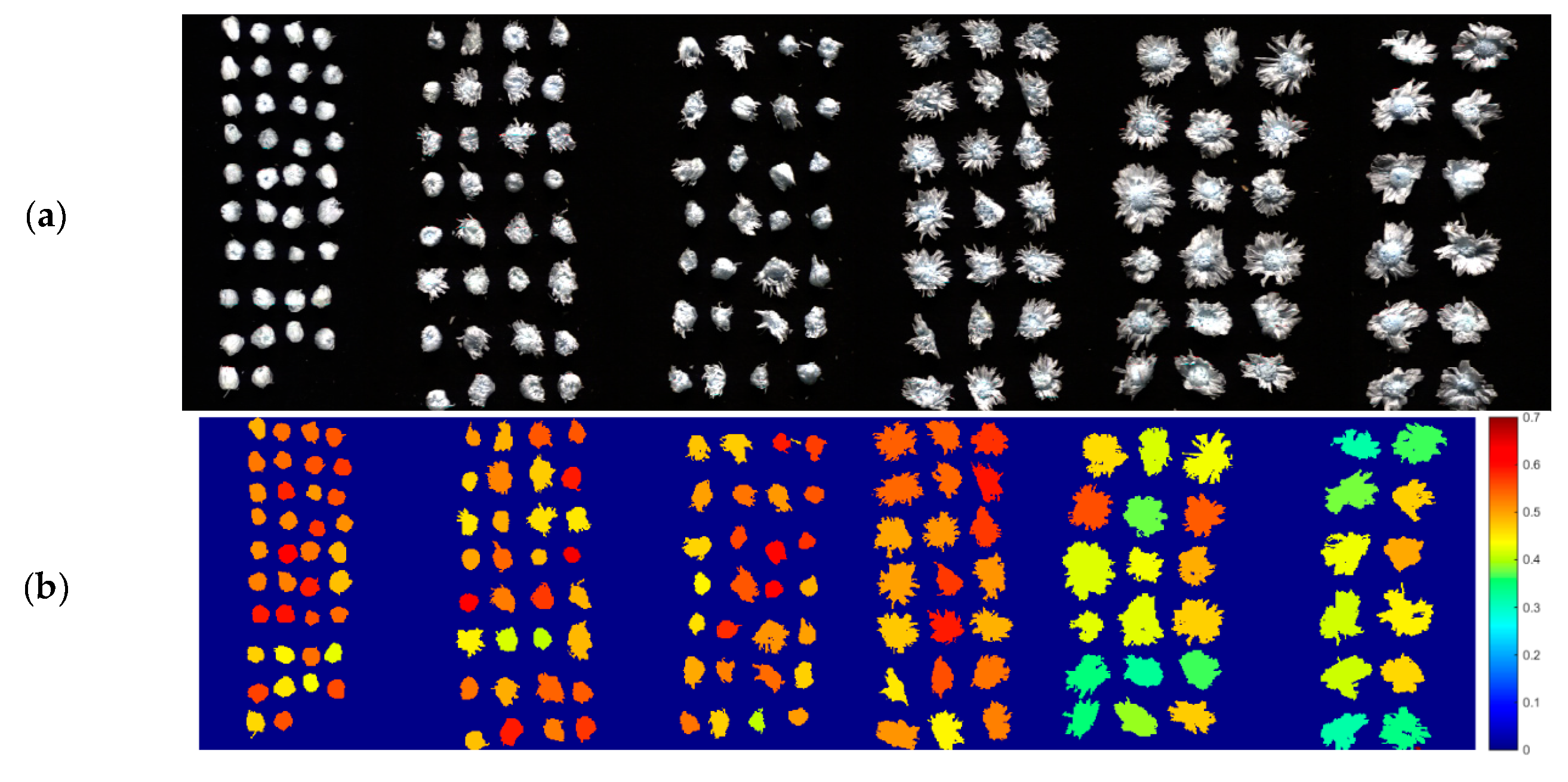
3.6. Visualization of Chlorogenic Acid, Luteolin-7-O-glucoside, and 3,5-O-Dicaffeoylquinic Acid in Chrysanthemum morifolium

As shown in Table 2 and Table 4, calibration models for chlorogenic acid, luteolin-7-O-glucoside, and 3,5-O-dicaffeoylquinic acid content determination obtained good results. These results illustrated the feasibility of using hyperspectral imaging to determine these chemical compositions. Based on the results, prediction maps for visualization of chlorogenic acid, luteolin-7-O-glucoside, and 3,5-O-dicaffeoylquinic acid content in fresh and dry Chrysanthemum morifolium flowers were formed. In general, ELM models using full spectra obtained better results for fresh and dry flowers. Thus, ELM models using full spectra were applied to construct the visualization maps for chlorogenic acid, luteolin-7-O-glucoside, and 3,5-O-dicaffeoylquinic acid in Chrysanthemum morifolium flowers. Based on the established models, these three chemical compositions content of each pixel within one flower could be obtained. Prediction maps by knowing pixelwise chemical composition content could be formed. However, for harvest, trade, and consumption, entire flowers were used rather than parts of each flower; knowing the average chemical composition content of all pixels within one flower would be more intuitive than knowing the distribution of pixelwise chemical composition content within one flower. Thus, average chemical composition content of each fresh and dry flower was visualized and the differences among flowers could be visualized. Figure 2 and Figure 3 show the prediction maps of chlorogenic acid, luteolin-7-O-glucoside, and 3,5-O-dicaffeoylquinic acid in fresh and dry Chrysanthemum morifolium flowers, respectively. As shown in Figure 2 and Figure 3, the size of flowers reduced after drying. With chemical compositions content presented by color, it would be possible to develop online detection systems or portable devices for rapid and accurate determination of chlorogenic acid, luteolin-7-O-glucoside, and 3,5-O-dicaffeoylquinic acid as well as other chemical compositions in fresh and dry Chrysanthemum morifolium flowers. The results would benefit the harvest, processing, and consumption of Chrysanthemum morifolium.

4. Conclusions

Near-infrared hyperspectral imaging coupled with multivariate analysis was used to determine chlorogenic acid, luteolin-7-O-glucoside, and 3,5-O-dicaffeoylquinic acid content in fresh and dry Chrysanthemum morifolium. Pixelwise spectra at the spectral range of 975–1646 nm were extracted and preprocessed by wavelet transform (WT) and area normalization. Successive projections algorithm (SPA) was used to select optimal wavelengths and the number of wavelengths reduced at least 95%. PLS, ELM, and LS-SVM models using full spectra and optimal wavelengths obtained good performances for both fresh and dry flowers, and most of the models had R²_c, R²_p over 0.80 and RPD over 2.00. Bias values of all models were small. These results indicated that hyperspectral imaging combined with multivariate analysis methods could be used to determine chlorogenic acid, luteolin-7-O-glucoside, and 3,5-O-dicaffeoylquinic acid content in fresh and dry Chrysanthemum morifolium flowers. In general, ELM performed relatively better than the other two calibration methods. For different chemical compositions, the models with the best performances were different, and the differences among different calibration methods were small. Statistically, these three calibration methods could all be used for chlorogenic acid, luteolin-7-O-glucoside, and 3,5-O-dicaffeoylquinic acid content determination in fresh and dry Chrysanthemum morifolium. Indeed, the performances were not satisfactory for real-world applications and the performances of the calibration models should be improved in future studies. Prediction maps of chlorogenic acid, luteolin-7-O-glucoside, and 3,5-O-dicaffeoylquinic acid content were obtained, and variations of these chemical compositions content among flowers could be found. The results would be helpful to develop rapid and nondestructive online quality detection and sorting systems or portable devices during the process of harvest, processing, and consumption of Chrysanthemum morifolium. In future studies, strategies to improve the model robustness and accuracy should be conducted. More calibration methods should be explored, and the optimal calibration method would be selected for real-world application.

References

1. Kaneko, S.; Chen, J.; Wu, J.; Suzuki, Y.; Ma, L.; Kumazawa, K. Potent Odorants of Characteristic Floral/Sweet Odor in Chinese Chrysanthemum Flower Tea Infusion. J. Agric. Food Chem. 2017, 65, 10058–10063. [Google Scholar] [CrossRef] [PubMed]
2. Mubarak, A.; Bondonno, C.P.; Liu, A.H.; Considine, M.J.; Rich, L.; Mas, E.; Croft, K.D.; Hodgson, J.M. Acute effects of chlorogenic acid on nitric oxide status, endothelial function, and blood pressure in healthy volunteers: A randomized trial. J. Agric. Food Chem. 2012, 60, 9130–9136. [Google Scholar] [CrossRef] [PubMed]
3. Kwon, Y. Luteolin-7-O-glucoside as a potential preventive and therapeutic candidate for Alzheimer’s disease. Exp. Gerontol. 2017, 95, 39–43. [Google Scholar] [CrossRef] [PubMed]
4. D’Antuono, I.; Carola, A.; Sena, L.M.; Linsalata, V.; Cardinali, A.; Logrieco, A.F.; Colucci, M.G.; Apone, F. Artichoke Polyphenols Produce Skin Anti-Age Effects by Improving Endothelial Cell Integrity and Functionality. Molecules 2018, 23, 2729. [Google Scholar] [CrossRef] [PubMed]
5. Commission, C.P. Chinese Pharmacopoeia; China Medical Science Press: Beijing, China, 2015. [Google Scholar]
6. Zhang, C.; Jiang, H.; Liu, F.; He, Y. Application of Near-Infrared Hyperspectral Imaging with Variable Selection Methods to Determine and Visualize Caffeine Content of Coffee Beans. Food Bioprocess Technol. 2017, 10, 213–221. [Google Scholar] [CrossRef]
7. Fan, S.; Li, J.; Xia, Y.; Tian, X.; Guo, Z.; Huang, W. Long-term evaluation of soluble solids content of apples with biological variability by using near-infrared spectroscopy and calibration transfer method. Postharvest Biol. Technol. 2019, 151, 79–87. [Google Scholar] [CrossRef]
8. Zhang, C.; Liu, F.; Kong, W.; Cui, P.; He, Y.; Zhou, W. Estimation and Visualization of Soluble Sugar Content in Oilseed Rape Leaves Using Hyperspectral Imaging. Trans. ASABE 2016, 59, 1499–1505. [Google Scholar]
9. Malmir, M.; Tahmasbian, I.; Xu, Z.; Farrar, M.B.; Bai, S.H. Prediction of soil macro- and micro-elements in sieved and ground air-dried soils using laboratory-based hyperspectral imaging technique. Geoderma 2019, 340, 70–80. [Google Scholar] [CrossRef]
10. Ortega, S.; Fabelo, H.; Iakovidis, D.K.; Koulaouzidis, A.; Callico, G.M. Use of Hyperspectral/Multispectral Imaging in Gastroenterology. Shedding Some-Different-Light into the Dark. J. Clin. Med. 2019, 8, 36. [Google Scholar] [CrossRef] [PubMed]
11. Sicher, C.; Rutkowski, R.; Lutze, S.; von Podewils, S.; Wild, T.; Kretching, M.; Daeschlein, G. Hyperspectral imaging as a possible tool for visualization of changes in hemoglobin oxygenation in patients with deficient hemodynamics—Proof of concept. Biomed. Eng./Biomed. Tech. 2018, 63, 609–616. [Google Scholar] [CrossRef] [PubMed]
12. Zhang, C.; Liu, F.; He, Y. Identification of coffee bean varieties using hyperspectral imaging: Influence of preprocessing methods and pixel-wise spectra analysis. Sci. Rep. 2018, 8, 2166. [Google Scholar] [CrossRef] [PubMed]
13. Lara, M.A.; Lleó, L.; Diezma-Iglesias, B.; Roger, J.M.; Ruiz-Altisent, M. Monitoring spinach shelf-life with hyperspectral image through packaging films. J. Food Eng. 2013, 119, 353–361. [Google Scholar] [CrossRef] [Green Version]
14. He, J.; Chen, L.; Chu, B.; Zhang, C. Determination of Total Polysaccharides and Total Flavonoids in Chrysanthemum morifolium Using Near-Infrared Hyperspectral Imaging and Multivariate Analysis. Molecules 2018, 23, 2395. [Google Scholar] [CrossRef] [PubMed]
15. Geladi, P.; Kowalski, B.R.J.A.C.A. Partial least-squares regression: A tutorial. Anal. Chim. Acta 1985, 185, 1–17. [Google Scholar] [CrossRef]
16. Huang, G.-B.; Zhu, Q.-Y.; Siew, C.-K. Extreme learning machine: Theory and applications. Neurocomputing 2006, 70, 489–501. [Google Scholar] [CrossRef] [Green Version]
17. Zhang, C.; Xu, N.; Luo, L.; Liu, F.; Kong, W.; Feng, L.; He, Y. Detection of Aspartic Acid in Fermented Cordyceps Powder Using Near Infrared Spectroscopy Based on Variable Selection Algorithms and Multivariate Calibration Methods. Food Bioprocess Technol. 2013, 7, 598–604. [Google Scholar] [CrossRef]
18. Araújo, M.C.U.; Saldanha, T.C.B.; Galvão, R.K.H.; Yoneyama, T.; Chame, H.C.; Visani, V. The successive projections algorithm for variable selection in spectroscopic multicomponent analysis. Chemom. Intell. Lab. Syst. 2001, 57, 65–73. [Google Scholar] [CrossRef]
19. Zornoza, R.; Guerrero, C.; Mataix-Solera, J.; Scow, K.M.; Arcenegui, V.; Mataix-Beneyto, J. Near infrared spectroscopy for determination of various physical, chemical and biochemical properties in Mediterranean soils. Soil Biol. Biochem. 2008, 40, 1923–1930. [Google Scholar] [CrossRef] [PubMed] [Green Version]
20. He, Y.; Zhao, Y.; Zhang, C.; Sun, C.; Li, X. Determination of ß-Carotene and Lutein in Green Tea Using Fourier Transform Infrared Spectroscopy. Trans. ASABE 2019, 62, 75–81. [Google Scholar] [CrossRef]
21. Jerry, W.; Lois, W. Practical Guide to Interpretive Near-Infrared Spectroscopy; CRC Press, Inc.: Boca Raton, FL, USA, 2007. [Google Scholar]
22. Frank, W.; Angela, S.; Martin, K. Incorporating Chemical Band-Assignment in near Infrared Spectroscopy Regression Models. J. Near Infrared Spectrosc. 2008, 1, 265–273. [Google Scholar]
Figure 1. Average spectrum with standard deviation of fresh and dry Chrysanthemum morifolium flowers. Bold lines are average spectra and vertical lines are standard deviation of each wavelength.
Applsci 09 01959 g001
Figure 2. Pseudo image of (a) fresh Chrysanthemum morifolium flowers and prediction maps of chlorogenic acid (b), luteolin-7-O-glucoside (c), and 3,5-O-dicaffeoylquinic acid (d). (Unit: % DW, DW means dry weight.)
Applsci 09 01959 g002
Figure 3. Pseudo image of (a) dry Chrysanthemum morifolium flowers and prediction maps of chlorogenic acid (b), luteolin-7-O-glucoside (c), and 3,5-O-dicaffeoylquinic acid (d). (Unit: % DW, DW means dry weight.)
Applsci 09 01959 g003aApplsci 09 01959 g003b