
Identification of Autism in Children Using Static Facial Features and Deep Neural Networks


1
School of Electronics Engineering, Vellore Institute of Technology, Vellore 632014, India
2
Department of Biomedical Engineering, Ajman University, Ajman P.O. Box 346, United Arab Emirates
3
School of Electrical Engineering, Vellore Institute of Technology, Vellore 632014, India
*
Author to whom correspondence should be addressed.
Brain Sci. 2022, 12(1), 94; https://0-doi-org.brum.beds.ac.uk/10.3390/brainsci12010094
Submission received: 31 October 2021
/
Revised: 3 January 2022
/
Accepted: 8 January 2022
/
Published: 12 January 2022
Abstract
:Autism spectrum disorder (ASD) is a complicated neurological developmental disorder that manifests itself in a variety of ways. The child diagnosed with ASD and their parents’ daily lives can be dramatically improved with early diagnosis and appropriate medical intervention. The applicability of static features extracted from autistic children’s face photographs as a biomarker to distinguish them from typically developing children is investigated in this study paper. We used five pre-trained CNN models: MobileNet, Xception, EfficientNetB0, EfficientNetB1, and EfficientNetB2 as feature extractors and a DNN model as a binary classifier to identify autism in children accurately. We used a publicly available dataset to train the suggested models, which consisted of face pictures of children diagnosed with autism and controls classed as autistic and non-autistic. The Xception model outperformed the others, with an AUC of 96.63%, a sensitivity of 88.46%, and an NPV of 88%. EfficientNetB0 produced a consistent prediction score of 59% for autistic and non-autistic groups with a 95% confidence level.
1. Introduction
Autism spectrum disorder (ASD) is a complex brain development disorder marked by restricted or repetitive activities, as well as social and communication difficulties. Autism is referred to be a “spectrum” disorder since the types and intensity of symptoms experienced by individuals differ greatly. The wide range of symptoms associated with ASD makes its diagnosis a difficult task. ASD affects people of all ethnic, racial, and socioeconomic backgrounds. Despite the fact that ASD is a lifelong illness, studies have shown that early detection and appropriate medical care can enhance a person’s long-term outcomes [1,2]. According to the Diagnostic and Statistical Manual of Mental Disorders (DSM-5) [3], individuals diagnosed with autism are likely to have difficulty interacting with others, poor oral communication skills, redundant behaviors, and an inability to perform daily activities at home, school, work, or in similar situations. One out of every 54 children in the United States has been diagnosed with ASD and boys are more likely than girls to be recognized as autistic, according to the Centers for Disease Control and Prevention (CDC) [4]. The American Academy of Pediatrics has suggested that all children have an early ASD screening test as part of routine health checkups to determine whether they should seek formal clinical diagnosis [1]. In June 2021, the World Health Organization (WHO) revealed epidemiological statistics indicating that ASD affects one in every 160 children worldwide; nevertheless, the incidence of ASD in many low- and middle-income countries remains unknown [5,6]. The development of reliable, easy-to-use, and cost-effective screening tools is crucial in light of the growing number of ASD cases and the associated costs of diagnosis and treatment. ASD diagnosis is problematic due to the lack of a single medical test that can accurately detect the disorder. To effectively diagnose ASD, doctors need to know the child’s developmental history as well as the presence of any ASD-related symptoms [1,2,7].
In various degrees, a parent, caregiver, or pediatrician may find ASD symptoms in youngsters for the first time. The specialist meets with the parent or caregiver to discuss the child’s developmental milestones and behavioral difficulties as the first stage of the diagnostic procedure. Following that, one or more conventional screening procedures based on DSM-5 diagnostic criteria are used to evaluate the child’s social and communicative abilities. Other tests, such as blood tests, electroencephalograms (EEG), and functional magnetic resonance imaging (fMRI), may be required for confirmation of the diagnosis, depending on the specialist’s recommendation [7,8,9]. Autism can be identified using cutting-edge equipment as early as two years of age; however, diagnoses are often delayed until after four years of age for a variety of reasons [10,11]. One of the major factors contributing to a delayed diagnosis is a shortage of highly skilled doctors, particularly in rural regions, who can recognize ASD signs in children and diagnose it swiftly. Furthermore, diagnosis is sometimes delayed due to a lack of access to the available ASD specialist. Delays in diagnosis might also be caused by the social, economic, and educational backgrounds of the parents [12,13,14].
The hunt for early-diagnosis neuromarkers is never-ending. Researchers have made several attempts to identify significant markers that can aid a specialist in the diagnosis of ASD. Some of the important markers now being examined are neurophysiological, behavioral, eye-tracking, anatomical and/or functional brain characteristics, and genetic [15]. Neurologists have recognized for a long time that facial dysmorphologies, or aberrant facial traits induced by abnormalities in the embryonic development process, are strongly linked to the underlying neurological issues. In 1964, when studying fetuses with holoprosencephaly (HPE), DeMyer et al. [16] coined the phrase “the face predicts the brain”. HPE is a serious condition that affects both the brain and the face. HPE presents itself in a variety of morphologies, according to DeMyer, ranging from the inability of the forebrain to divide into right and left lobes to normal partitioning. These findings highlight the fact that the brain and the developmental mechanisms that shape the face are inextricably linked, implying that changes in one might have a significant impact on the other. Autism spectrum disorders (ASDs) are caused by anomalies in the embryological brain, as evidenced by the fact that newborns with ASD have facial development that differs significantly from that of typically developing children [17,18]. Some of the frequent facial features of autism are a broader upper face, shorter middle face, wider eyes, bigger mouth, and the philtrum [19].
The use of facial features as a physical marker to detect autism is one of the most exciting topics in autism research. This method necessitates exact measurements of the distance between pairs of facial landmarks and protrusions in order to quantify the child’s facial asymmetry. The predicted dysmorphology scores definitely demonstrate ASD. Obafemi et al. [20] used the 3dMD face system, which includes a 3D camera that captures hundreds of facial images in the x, y, z dimensions. The pictures are then combined into a 3D surface mesh, which allows for Euclidean facial shape measurements down to the millimeter level [21]. According to Miles and Hillman [22], there were significant differences in facial morphology between children with ASD and typically developing (TD). The findings also reveal that people with ASD can be divided into subgroups based on their facial features. Membership in each of these distinct groups was also highly associated to clinical and behavioral characteristics.
Miles and Hillman [21] devised a classification system that divides children into two groups, complex and essential, depending on the number of minor physical defects (MPAs). Children with ASD who were dysmorphic (six or more MPAs) with or without microcephaly were defined as having “complicated” autism and were more likely to have genetic disorders, anatomical abnormalities in the brain, seizures, and a low IQ. The remaining children were labeled as having “essential” autism because there was no evidence of an early embryological abnormality [22]. Later, the researchers created the autism dysmorphology measure (ADM), which can be used to quickly screen for complicated autism without requiring a naked examination. Photographs of each child were examined to evaluate the authenticity of the findings [23].
Angkustsiri, K. et al. [24] investigated the possibility of using facial photography analysis to assess generalized dysmorphology. This study included 324 children aged 2 to 5 years old with ASD, developmental deficits, and TDs. To classify the photos into subgroups (dysmorphic or non-dysmorphic), the researchers performed a physical examination to evaluate the number of MPAs in the children, with a threshold of 3 or more for dysmorphic. According to the study, children with ASD are more dysmorphic than children without ASD (p = 0.007). Photographic examination can be used to detect generalized dysmorphology in children, which could be a symptom of ASD, according to the findings. Some of the most important limitations for extracting MPAs from child pictures are as follows:
- (a)
- Manually evaluating 2D face photographs is time-consuming, labor-intensive, and prone to bias and inaccuracies.
- (b)
- A 3D camera would be great for this work, but it is expensive.
- (c)
- Specialized algorithms running on powerful computers are another prerequisite for automata.
In recent years, machine learning (ML) methods have gained prominence in a variety of domains, including picture classification [25,26,27]. Because of their amazing capacity to learn from hidden patterns acquired from enormous volumes of data, machine learning algorithms can be an effective predictor. A feature extractor plus a machine learning algorithm make up an ML-based image classifier. The convolutional neural network (CNN) is the most often used feature extractor, and there are a range of machine learning methods to pick from to find the one that best fits the data.
Tania et al. [27] were the first to publish a peer-reviewed paper titled “A transfer-learning-based autism classification model utilizing 2D face photos”, according to our understanding. To categorize the input image as autistic or usually developing, the researchers created an ML classifier. The researchers used an open-access Kaggle face picture dataset with 2936 face photographs of 1468 children with ASD and 1468 children with TDs. To find the best performing classifier, experiments were conducted on a variety of machine learning and deep learning classifiers. According to the results, the MobileNet-V1 had the greatest test accuracy of 90.67 percent. The researchers hope to increase the model’s overall accuracy in the future.
Children with autism have different facial features than age and gender-matched TDs, as evidenced by the literature cited above. Furthermore, CNN’s ability to identify images may be effective in the early detection of ASD in youngsters. Considering the aforementioned observations, we set our goal to construct an optimal CNN-based model that can accurately diagnose autism in children with maximum sensitivity and specificity utilizing characteristics extracted from face photos. We utilized the MobileNet model as a baseline to compare the performance of the other two models, Xception and EfficientNets.
2. Materials and Methods
The dataset, detailed methodologies adopted, testing the model, and metrics used to evaluate the model’s performance are described in this section. The algorithms were developed and run using Google Colab in the python language (Colaboratory). Google launched the Colaboratory to promote machine learning research, which offers a cloud-based Jupyter notebook environment that requires no setup and is available for free. An Intel(R) Core (TM) i7-10750H CPU with a Dell XPS 15 9500 model laptop @ 2.60 GHz, 2592 MHz, 6 Core(s) and 12 Logical Processor(s) were used as local runtime.
2.1. Dataset
The lack of an open-access and large image dataset, which is a requirement for creating ML-based image classification models, was one of the most crucial obstacles in our research work. To create our suggested models, we used the autistic children dataset from the Kaggle repository [28], which is, as far as we know, the first and only dataset of its sort. The dataset includes 2936 colored 2D face photos of children ranging in age from 2 to 14, with the majority of them lying between the ages of 2 and 8. The gender distribution in the autistic class (male vs. female) was roughly 3:1, whereas the ratio in the TD class was approximately 1:1. The dataset lacks some information, such as the child’s clinical history, ASD severity score, ethnicity, and socio-economic background. The dataset is divided into three folders: training, valid, and test, each with two subfolders: autistic and non-autistic. The training set has 2536 images, the validation set included 100 images, and the test set contains 300 images split evenly between the subfolders. Ideally, the training set for the ML model should have an exceptionally rich collection of images that encompasses the entire spectrum of the ASD to achieve an accurate and consistent result. In practice, image classifier algorithms based on machine learning require training using tens of thousands of images. In comparison to other image datasets, the size of the existing dataset is quite small.
2.2. Model Building
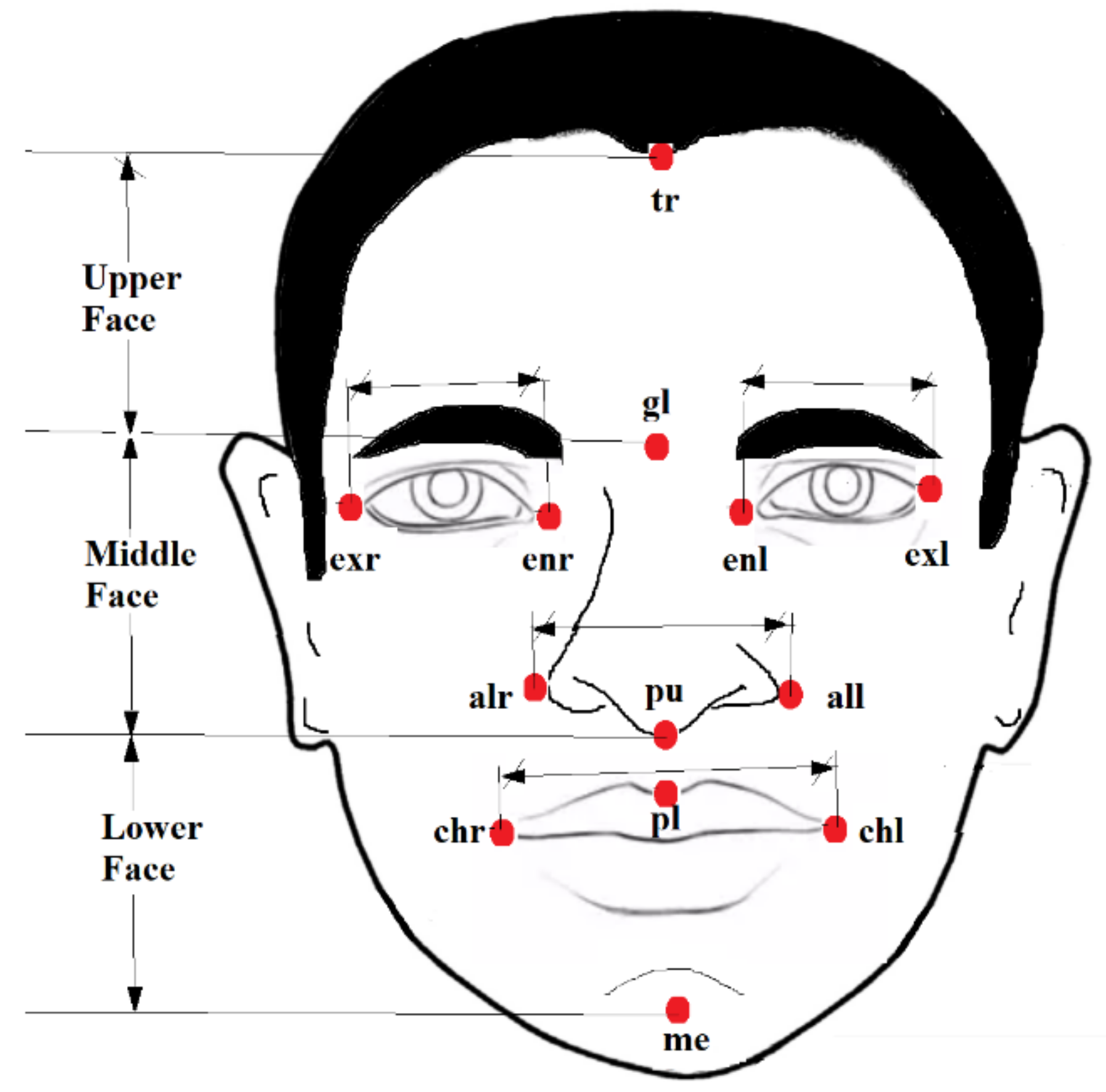
Figure 1 depicts a number of facial landmarks on the three segments of a human face, namely the top face, middle face, and lower face. A specialist scarcity can use the Euclidean distance between the landmarks to determine the degree of face dysmorphology (if any) present in the child. A list of the most essential ASD relevant facial anthropometric measures are included in Table 1. A broader top face, a shorter middle face, wider eyes, a wider mouth, and a philtrum are some of the common facial features seen in children with ASD [16,17]. In a recent study, researchers employed a 3dMD camera to obtain these measurements directly from children; however, the 3dMD camera system is costly, and the method is time-consuming. In our research, we employed machine learning algorithms to extract a variety of facial metrics from each of the training images in a fraction of a second.
To extract distinct attributes from the input photographs, we employed a CNN-based feature extractor with a series of digital filters. Each of these filters contains a set of learnable parameters (called weights and biases) to capture salient features from the training images. The digital filters used in our model can collect elements such as edges (horizontal, vertical, inclined), contours, curves, and corners available in the photos using various combinations of weights and biases; such a task is hard to carry out by visual analysis by an expert. As mentioned in the introduction, this proposed model primarily has two modules, a feature extractor, and a classifier. We use pre-trained ML models as feature extractor and a deep neural network as the classifier. Because of their subtlety, the proposed models may automatically perform robust feature extraction to the point where it is nearly impossible to detect by simple observation. For training, validating, and testing the models, the suggested methodology requires the organization of image data into train, validation, and test sets. The test scores are used to evaluate the model’s performance.
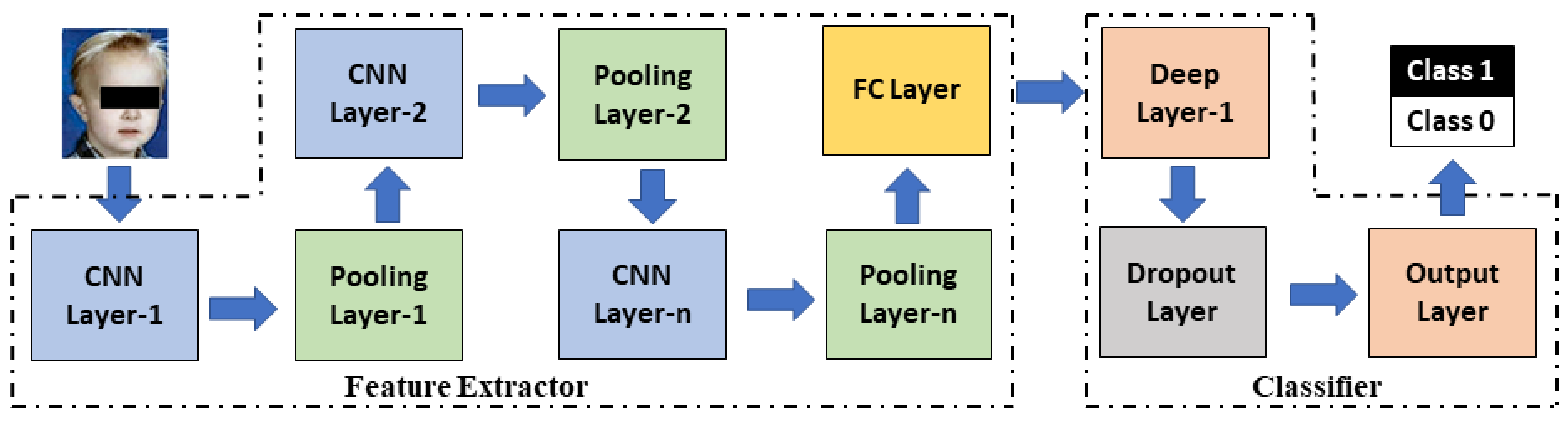
As illustrated in Figure 2, the feature extractor module consisted of a series of convolutional and pooling layers [29,30,31,32]. Convolutional layers are in charge of executing a mathematical operation known as convolution, which is an image filtering technique that aids in the extraction of multiple features from an input image [29,30]. Equation (1) explains the mathematical implementation of the convolution, where f(x, y) is the input image pixel, w(x, y) is the filter mask, and g(x, y) is the resultant output image [32]. Convolution is accomplished by applying a filter mask (of size 3 × 3 or 5 × 5) to each pixel in the input image, yielding a feature map as a result. The dimension (W_conv) of a convolved image corresponds to an input image I of size (height, H x width, W* channels, C), using K filter masks each of size (M rows × M columns), with zero-padding Z and stride S is estimated using the Equation (2). As previously stated, each filter mask has particular weights and biases associated to it, collectively known as learnable parameters, which define the nature of the generated features. Model training begins with some default parameters, which are updated as the workout progresses [31]. The parameters, P_conv of a convolutional layer, are obtained using (3). In practice, an accurate image classifier demands the employment of many filters in order to have the greatest number of distinct features, resulting in a significant increase in the dimension of feature maps. Pooling layers are used to lessen the problem by eliminating redundant data from feature maps. Equation (4) gives the output of a max-pooling layer (W_pool) [32]. The max-pooling layer has no parameters associated with it. The feature extractor module outputs a fully connected layer (FC layer), which is responsible for reshaping the feature map as needed for the classifier module. Equation (5) determines the number of parameters (P_fc) associated with the FC layer with N neurons. Finally, a deep neural network (DNN) classifier is utilized to produce a prediction at the output. An input layer, hidden layers, and an output layer make up the DNN module.
In recent years, many efficient pre-trained image classifier algorithms have been developed and made available for research, owing to the efforts of the machine learning developer communities [33,34,35,36,37]. A pre-trained model has been trained to solve a problem similar to the one in hand using a large benchmark dataset. Rather than starting from scratch, a pre-trained model gets the model weights and parameters by transfer learning, resulting in more accurate models in less time [36,37]. We adopted five pre-trained models in the proposed work: MobileNet, Xception, EfficientNetB0, EfficientNetB1, and EfficientNetB2 as feature extractors, and experimented to find the best model for ASD prediction. The models we used in our research are the best-performing models, demonstrating great performance in image classification tests due to their ability to extract many features without sacrificing computing efficiency. The basic configuration and essential features of the models are described below.
2.3. Feature Extractors Used
2.3.1. MobileNet
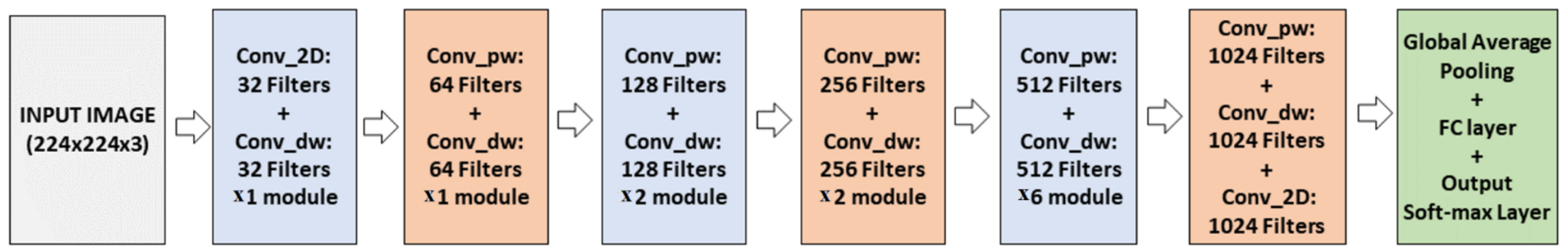
MobileNet is a CNN model designed to perform image classification efficiently on mobile devices, embedded systems, or low-power computers without a GPU [38]. The architecture of the MobileNet model is presented in Figure 3. This model is distinguished from other CNN models by the presence of depth-wise separable filters which combine a depth wise convolution (conv_dw) and pointwise convolution (conv_pw).
Unlike standard convolution, depth wise convolution exploits each channel of the input image separately to extract feature maps using different filter methods. Filter masks of size (1 × 1) are used to increase the number of channels in the output image to the required extent, resulting in a significant reduction in computational load. The MobileNet model has 3,364,930 parameters in total, 3,340,738 of which are trainable and 24,192 of which are non-trainable. This model is known for being a simple deep neural network. Object detection, face attribute identification, fine-grain classification, and geographic localization are just a few MobileNet applications.
2.3.2. Xception
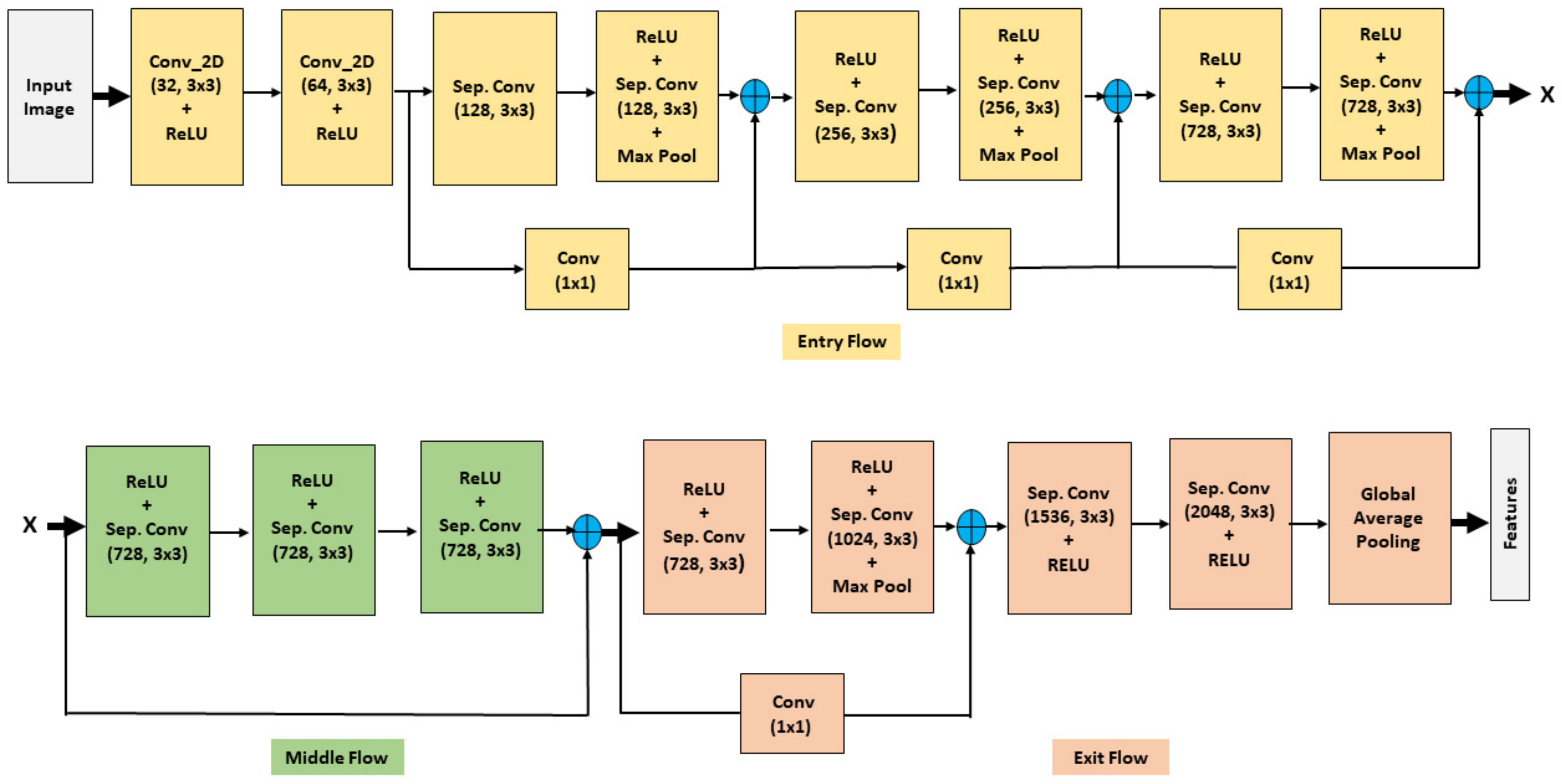
Google’s Inception model inspired the Xception [39] model, and it has a simple and modular architecture. The Xception model has three compartments: entry, middle, and exit, as shown in Figure 4. A linear stack of depth-wise separable convolution layers has been max-pooled with residual connections in each compartment. The input image (standard image size: 299 × 229 × 3) first goes through the entry flow and output X with 19 × 19 × 728 feature maps, as marked in Figure 4. The data X passes through the middle flow eight times and produces a feature map of 19 × 19 × 728 before passing through the exit flow. The output of the exit flow carries 2048 features for a standard size input image. The model has an optional FC layer and logistic regressor, which are not shown in the Figure.
There are 21,073,834 trainable and 58,800 non-trainable parameters in the Xception model, totaling 21,132,714 parameters. The Xception model is a heavy model that requires more computer resources due to the increased parameters.
2.3.3. EfficientNet
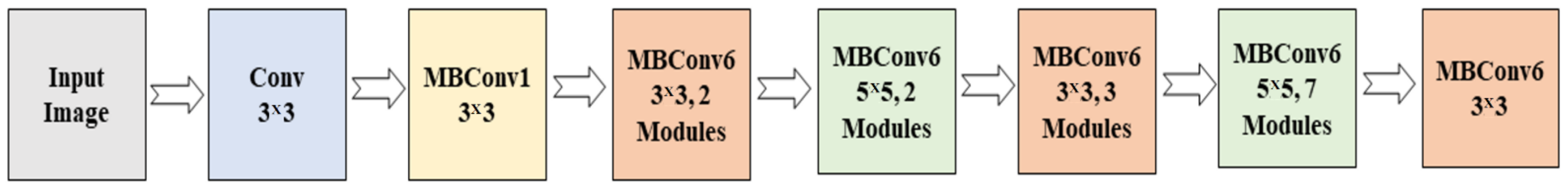
EfficientNet is one of the most efficient models that achieves state-of-the-art accuracy on both image-net and common image classification tasks, as first introduced by Tan and Le in 2019 [40]. EfficientNet has a CNN architecture and scaling method that uses a compound coefficient to uniformly scale the depth/width/resolution dimensions instead of standard practice, which scales these factors arbitrarily. According to intuition, as image resolution improves, the network’s depth and width should also improve. Larger receptive fields can capture similar features that include more pixels in an image as the depth is increased. The EfficientNet has a family of models (B0 to B7 with B0 being a baseline model) representing a good combination of efficiency and accuracy on various scales by introducing a heuristic way to scale the model. The EfficientNet architecture uses mobile inverted bottleneck convolutions in addition to standard convolutions (MBConv) as shown in Figure 5. An MBConv Block is a residual block that uses an inverted structure for efficiency in image classification models. It was first found in the MobileNetV2 CNN architecture and has since been used in several mobile-optimized CNNs.
The number of model parameters is the main difference between the eight EfficientNet variants. Total trainable parameters for models B0, B1, and B2 are 4,219,429, 6,745,097, and 7,955,323, respectively, with non-trainable parameters of 4,174,590, 6,680,226, and 7,884,676. We tested all EfficientNet variants to see how well each model performed overall on the given dataset.
2.4. Classifier Module
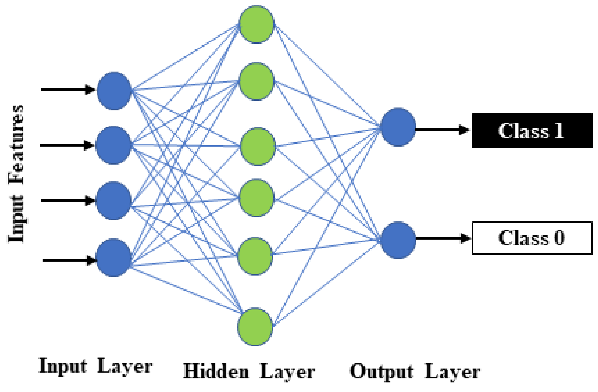
Using the thousands of features gathered by the feature extractor modules, we used a DNN classifier to make predictions. This module has three layers: an input layer that receives features from the previous layer (FC layer), a hidden layer with 256 neurons, and an output layer with a sigmoid activation function to make binary predictions [41]. A dropout layer with a drop rate of 0.5 is added between the dense and output layers to improve the model’s regularization [42]. Figure 6 depicts the various layers and their connections.
2.5. Model Training, Validation, and Test
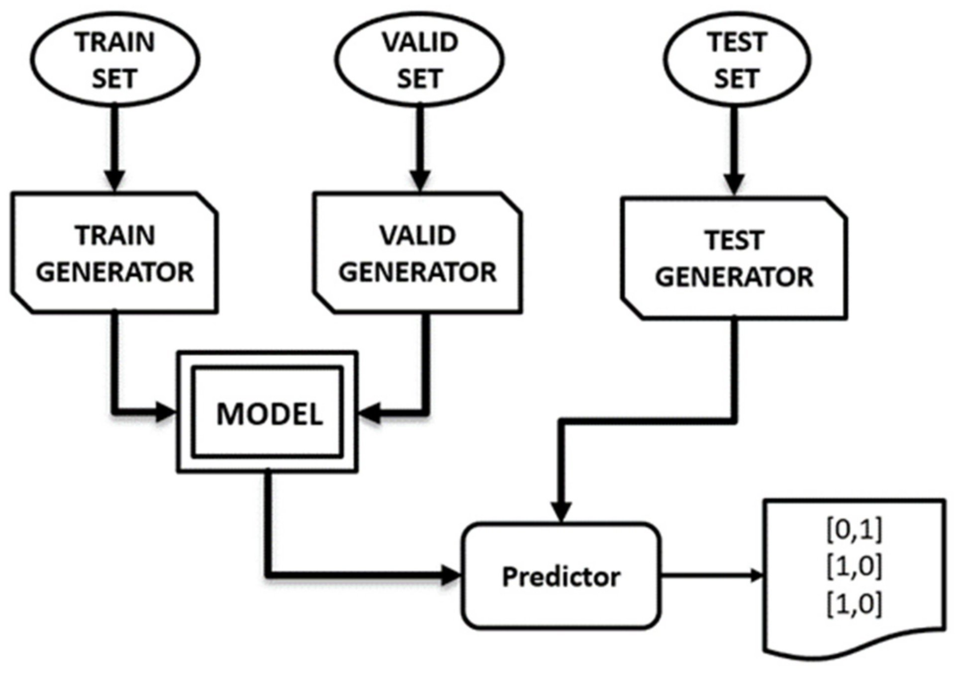
To build any ML model, the empty model must be trained and validated using a dedicated set of train and validation images, respectively. This is followed by testing the model using a set of previously unseen images (test images) in order to estimate the model’s performance. Training and validation datasets contain images with distinct labels indicating the class (autistic or TD) to which each image belongs, while test images lack labels. The trained machine learning model retains critical features extracted from the training images and is capable of accurately predicting the class of any unknown data (new data) using the learned knowledge. As a result, a well-trained machine learning model for ASD screening can accurately predict a child’s class, based on his face photo. As shown in the data flow diagram given in Figure 7, we used three data generators: train generator, validation generator, and test generator, to flow images as batches from the image folder as part of training, validation, and testing of the five proposed ML models. At first, we trained each model using the training set that has 2536 photographs (in two classes), then these model’s performances were validated using 100 photos (in two classes). Finally, we used 300 test images to evaluate the performance of the predictor.
2.6. Model Compilation and Hyperparameter Settings
We compiled the models using “Adam” as an optimizer, binary cross-entropy as a loss measure, and accuracy as a metric score. Experimentally, we discovered the following hyper-parameters to be the most effective: The learning rate 0.001, the batch normalization momentum 0.9, the batch size i64, and the number of epochs 30.
2.7. Measure of Model’s Performance
We choose the following metrics to evaluate the models: specificity (Spec.), sensitivity (Sens.), negative prediction value (NPV), positive prediction value (PPV), and AUC (area under ROC curve). We calculated the first four measures using a confusion matrix using Equations (6)–(9). The confusion matrix has four cells with designations: true positives (TP), false positives (FP), true negatives (TN), and false negatives (FN) [43].
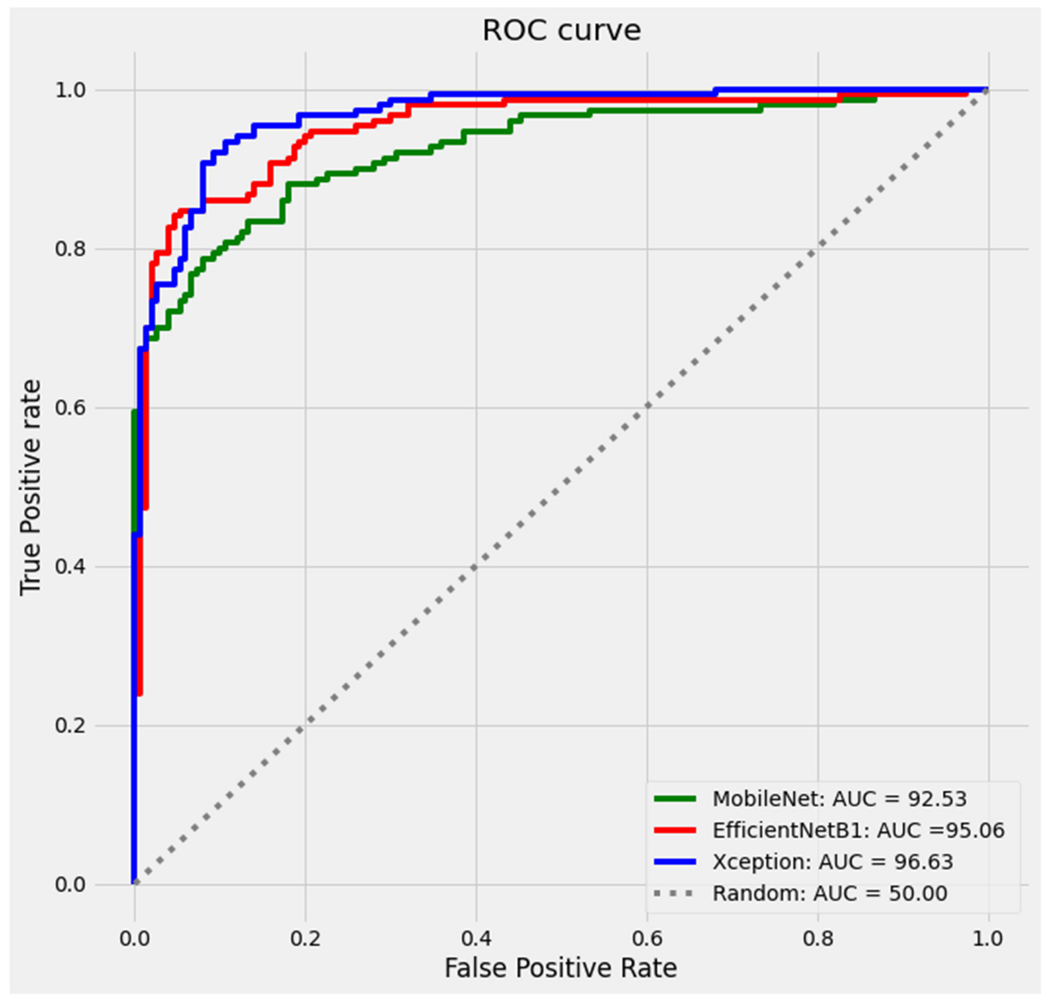
The AUC was calculated using a receiver operating characteristic (ROC) curve. The ROC is a TP vs. FP plot that shows a binary classification model’s performance at various classification thresholds [44]. In medical image classification problems, AUC is favored over accuracy (calculated from the confusion matrix) since the accuracy metric does not reflect the probability of the prediction, and the class with the highest likelihood of estimation is the same as the target. Furthermore, the model’s accuracy is influenced by the size of the test data. When the test data is small, AUC is a superior measure of accuracy, according to the research [45].
3. Results
We used the data flow generators to feed the data to the model in batches to train and validate each of the five proposed models, MobileNet, Xception, Effi-cientNetB0, EfficientNetB1, and EfficientB2, as mentioned in the preceding section. There were 2536 images in the training set (1268 autistic and 1268 TDs), and 100 images in the validation set (50 autistic and 50 TDs). The default model settings and hyperparameters provided in the previous section served as our starting point. We repeated the training cycles with different hyperparameters until we achieved the best results.
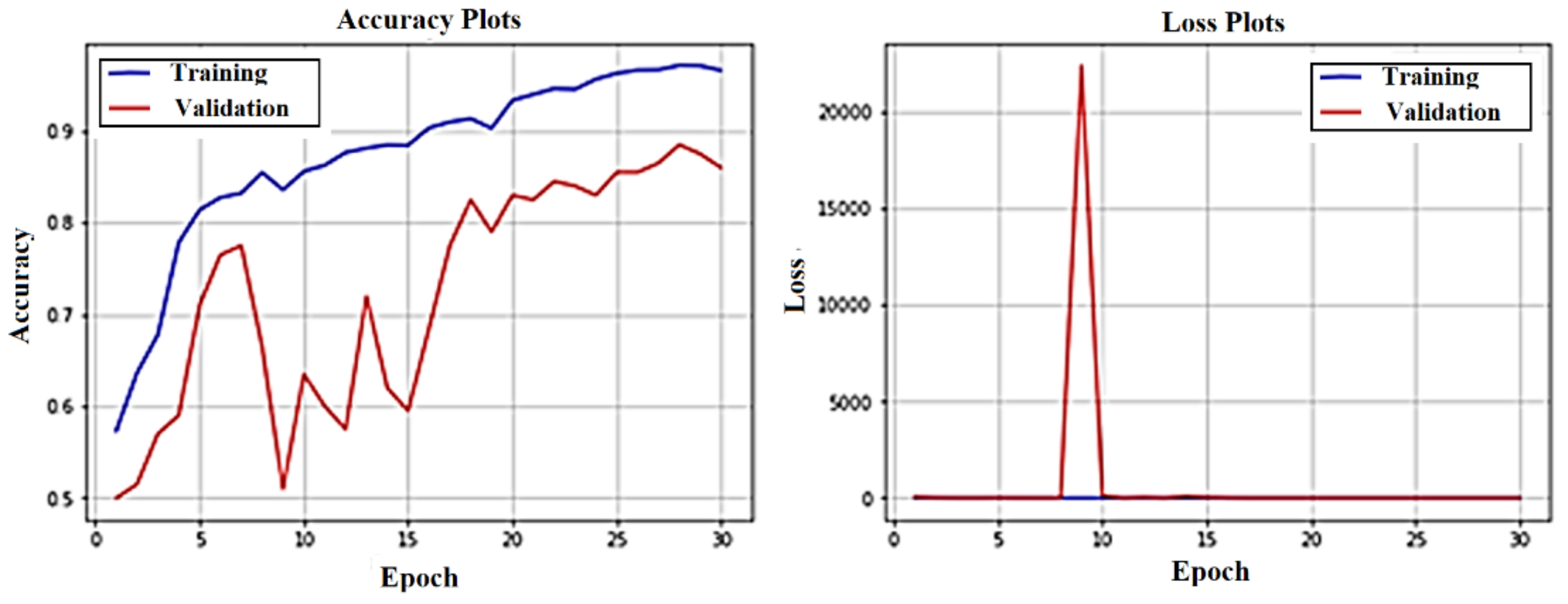
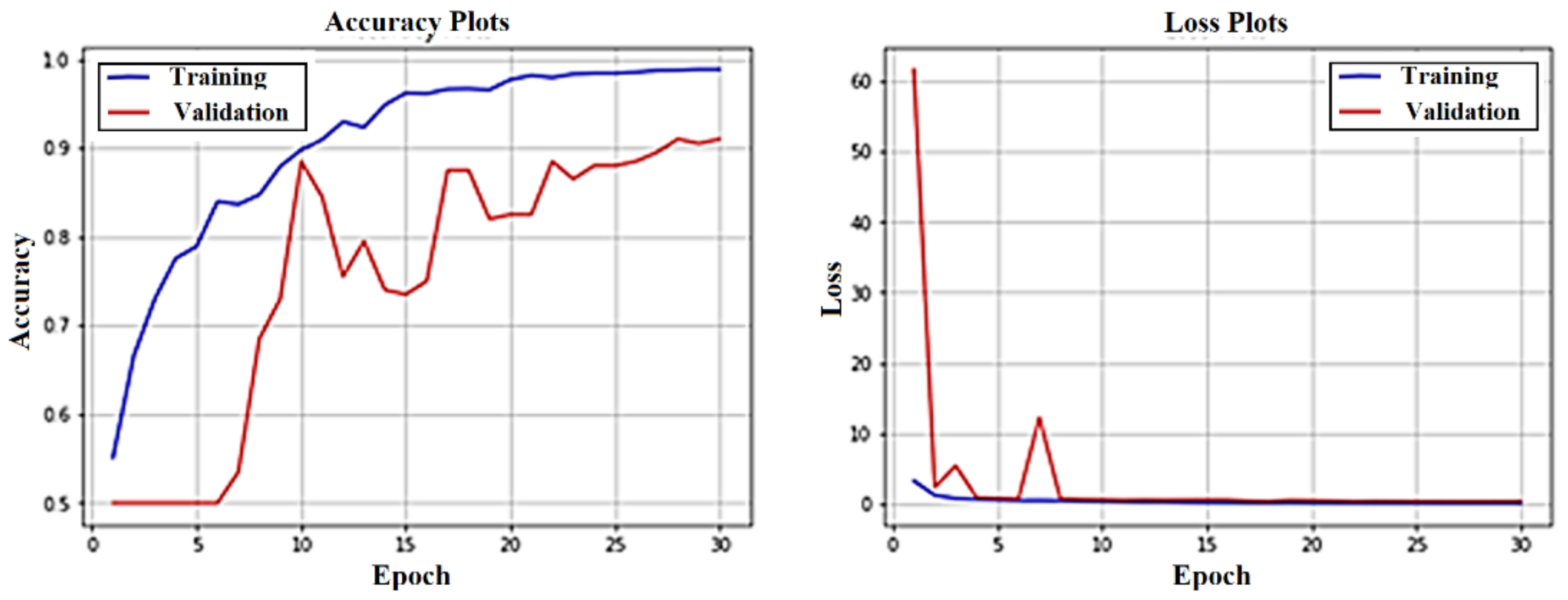
The accuracy and loss curves for the MobileNet, Xception, and EfficientB1 training and validation are shown in Figure 8, Figure 9 and Figure 10. The fit of each model to the training and validation data is represented by these curves.
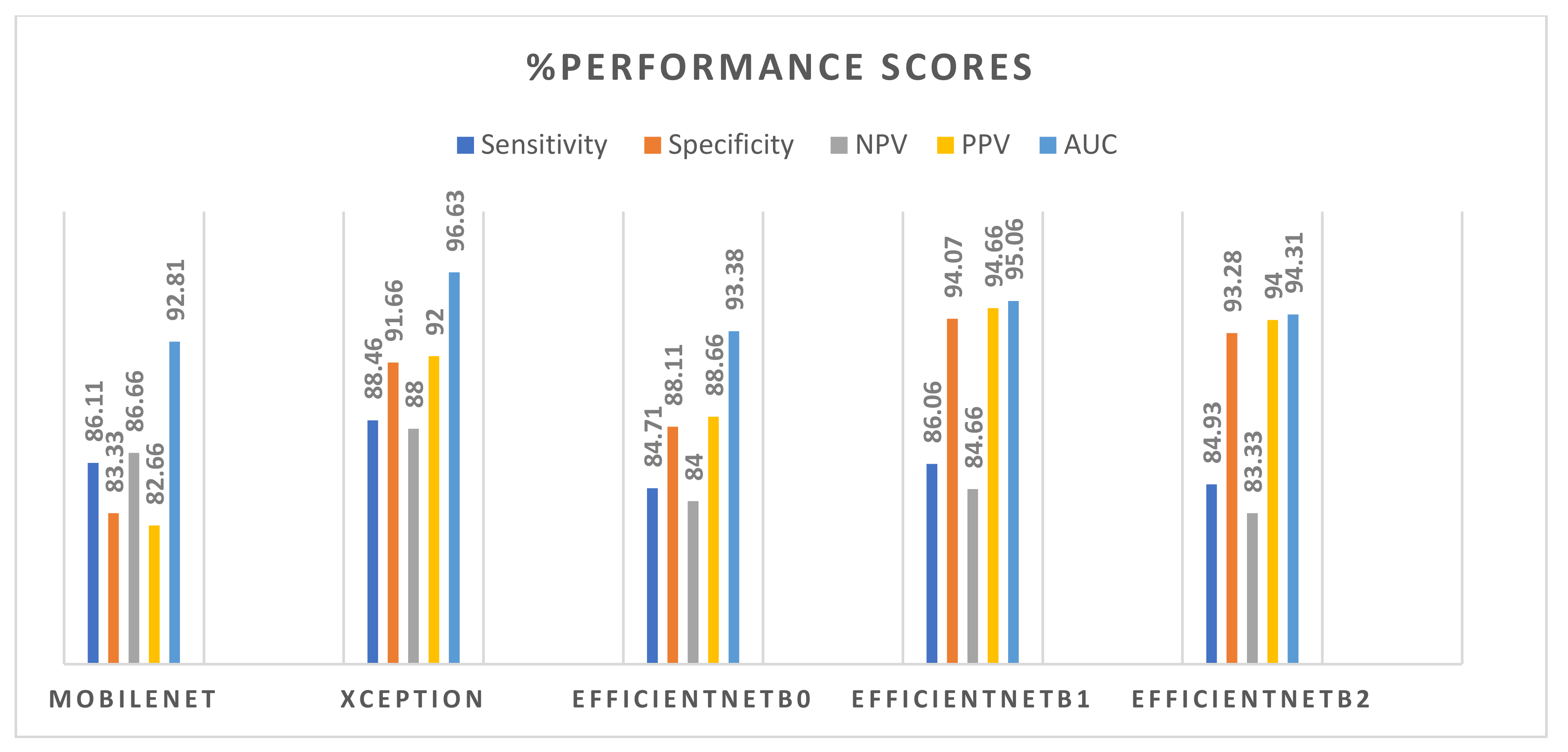
Using Equations (5)–(8), we determined the performance measure sensitivity, specificity, PPV, and NPV for each model on test data, as well as estimating AUC values from ROC curves. Table 2 summarizes the performance scores of the five models used in our research study. We used the MobileNet as a baseline model, with the following scores: 86.11% sensitivity, 83.33% specificity, 86.66% NPV, 82.66% PPV, and 92.81% AUC.
Table 2 shows that the Xception model outperformed the MobileNet model across the board, with scores of 88.46% sensitivity (2.67% improvement compared to baseline model), 91.66% specificity (9.99% improvement), 88.00% NPV (1.54% improvement), 92.00% PPV (11.29% improvement), and AUC of 96.63% (3.82 % improvement). However, other models, as shown in the table, outperformed in a few but not all metrics. The best three ROC curves are presented in Figure 11. Figure 12 compares the performance of the five models in terms of sensitivity, specificity, PPV, NPV, and ROC.
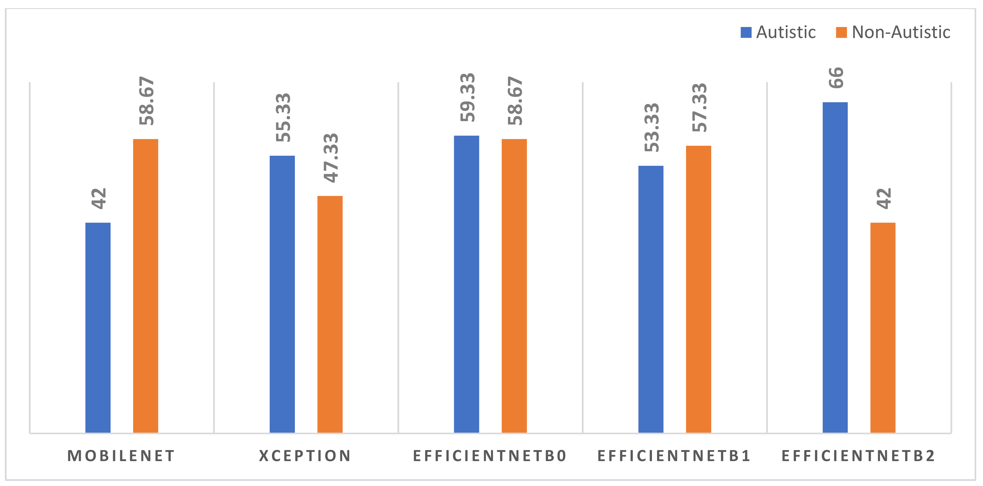
The models yielded a prediction rate for each case, which indicates the probability that each child will be classified as autistic or not. On the 300 test data samples, Table 3 shows the prediction rates of the five models (only five records from each class are included in Table 3). We devised a new scoring method for autistic and TD children based on class probabilities with a threshold of 95%. According to the scoring methods, if a model’s prediction meets the threshold, it receives one point. A comparison of model performance based on the new scoring is shown in Figure 13. The EfficientNetB0 showcased consistent scores of 59.33% for autistic class and 58.67% for TD class.
4. Discussion
The goal of this research was to develop a CNN-based model that can accurately predict autism in children using photos of their faces. We have reviewed the currently used autism diagnosis tools, also the main reasons for late diagnosis. We agree that there are numerous impediments to early diagnosis, referrals, and treatment, particularly among children from low-income families. The paucity of an adequate number of well-trained specialists is one of the key hurdles to early ASD diagnosis. Another big challenge is heterogeneity in the symptoms of ASD. We built five pre-trained CNN models that could be used as ASD classifiers (the MobileNet, Xception, and three variants of EfficientNet: EfficientNetB0, EfficientNetB1, and EfficientNetB2). The Xception model scored the highest AUC (96.63%), sensitivity (88.46%), and NPV (88%), while the EfficientB1 model achieved the highest specificity (94.07%), and PPV (94.66%). EfficientNetB0 outperformed the other models in the study, with an efficiency of 59.33% for autistic data and 58.67% for TD children. According to the statistics, the EfficientB0 is the only model that consistently predicts the class of any unseen test image with a confidence level of 95% or above. To ensure that the EfficientB0 model’s diagnoses are correct, we must test it with a reliable dataset that includes images of autistic and TD children identified by an expert using any standard ASD diagnosis technique that incorporates DSM-5 criteria.
Using datasets such as ImageNet, CIFAR, and others, the pre-trained CNN-based image classification algorithms that apply transfer learning have achieved excellent accuracy of over 90% (top-1 accuracy) and over 98 percent (top-5 accuracy) in recent years [30,31,32]. With over 14 million images organized into over 21,000 categories, ImageNet is a vast library of annotated photographs. ImageNet has become a benchmark dataset for image classification algorithms due to its image diversity and size. Autism identification using face photos, unlike conventional image classification systems, is a delicate subject. The consistency and overall quality of the photographs used to train these models have a significant influence on their performance. From the photos in the training set, the model should be able to distinguish as many ASD-related face traits as feasible. Some of the frequent facial signs of autism are a broader upper face, shorter middle face comprising cheeks and nose, wider eyes, bigger mouth, and the philtrum as mentioned in the introduction. Because the above characteristics are intimately linked to face emotions, only a facial image with a neutral feeling can offer these details precisely. The findings of the experiments showed that images with a neutral sense obtain higher accuracy. As a result, when training the CNN-based ASD classifier with face photos, it is ideal to use neutral emotion facial images. To ensure appropriate head alignment, the images must be taken with the child’s eyes open and visible (no hair blocking the eyes) on a plain light-colored background, with both ears visible. The shot must be taken in a consistent lighting environment with no shadows or flash reflections, as well as adequate brightness and contrast.
Only a few research articles have been published on the issue, and it is claimed that one of the primary obstacles for the few studies that have been undertaken is a dearth of open access datasets. Our suggested Xception model outperformed a recently published study [27], which employed the same dataset and obtained an AUC of 90.67% using a MobileNet model. However, in comparison to the MobileNet and EfficientNet, a significant number of model parameters necessitate the use of the Xception, making it a computationally expensive model.
Following a thorough review of the dataset utilized in our research, we discovered the following issues: inconsistent image quality and the absence of critical information such as child’s age, gender, and autism score. As a result, in the future, we want to gather photographs of autistic children with standard picture quality, as well as metadata from reputable sources such as autism diagnostic centers or affiliated pediatric clinics. As a future project, we plan to investigate how to predict ASD severity score using the facial features of children diagnosed with ASD.
Early ASD screening with face photographs will have a big impact on the child, his or her parents, and the clinician. In terms of the advantages of early ASD diagnosis, after providing the child’s face photograph, the doctor just needs a few seconds to determine if the child is autistic or TD. Furthermore, the model gets greater accuracy as it is trained on a bigger training set; nevertheless, the situation becomes more difficult when an expert manually diagnoses a child as autistic or TD based on visual interpretation of facial traits. In addition, if the proposed model is made available as a mobile application, a parent can administer the screening exam on their own, which will aid them in preparing referrals or diagnostic tests. While our approach has some advantages, it also has some disadvantages, such as a high rate of false positive (FP) and false negative (FN) results. FP can result in a misdiagnosis, resulting in unnecessary medical procedures and parental concern. A large percentage of false negatives, on the other hand, leads to missed diagnoses and treatment delays. As a result, it is important to remember that the suggested method will not be able to diagnose ASDs on its own; rather, the results will need to be clinically compared with results from other techniques like QCHAT, ADOS, and others.
We computed performance scores by running the model one at a time. We employed optimization tactics for individual models to enhance accuracy, which included adjusting hyperparameters such as batch size, number of epochs, and learning rate, among other things. In order to improve model scores, we would like to use an ensmenble approach in the future.
With the help of anomaly filters, the suggested models will increase their accuracy even higher. Before the model is trained, an image anomaly filter is applied to the training dataset, thereby excluding unsuitable images from the dataset. When compared to current parent-administered screening approaches for early ASD screening, the proposed method would have a beneficial influence on ASD diagnosis because it is simple, rapid, and accurate. However, clinical validation of the suggested models will require additional testing and evaluations with a dataset that accurately replicates real-world settings.
5. Conclusions
This study looked into the utility of facial features as a biomarker for accurately distinguishing autistic children from TD children. We used a publicly available dataset that included face images from both children (ASD and TD). Five CNN-based binary ASD classifier models that use five pre-trained models, MobileNet, Xception, EfficientNetB0, EfficientNetB1, and EfficientNetB2, were built and tested to evaluate the scores of each model. We discovered that the Xception model outperformed the other models and achieved an AUC of 96.63%, a sensitivity of 88.46%, and an NPV of 88.00%. When we compared the detection rates of each model with a 95% confidence level, the EfficientB0 received the highest scores: 59.33% for autism class and 58.67% for TD class. The findings show that the distinct features of ASD can be efficiently gathered from static face images of a child, allowing for a quick and accurate ASD screening method.
Author Contributions
Conceptualization, methodology, coding, analysis and original manuscript preparation, K.K.M.R.; supervision, review manuscript and project administration, M.M.S. All authors have read and agreed to the published version of the manuscript.
Funding
This research received no external funding.
Institutional Review Board Statement
Not applicable.
Informed Consent Statement
Not applicable.
Data Availability Statement
The data used in this paper is publicly accessible, and details are available in the references section.
Conflicts of Interest
The authors declare no conflict of interest.
References
- National Institute of Mental Health. Autism Spectrum Disorder. Available online: https://www.nimh.nih.gov/health/topics/autism-spectrum-disorders-asd/#:~:text=Autism%20spectrum%20disorder%20(ASD)%20is,first%20two%20years%20of%20life (accessed on 10 September 2021).
- Bölte, S. Is autism curable? Dev. Med. Child Neurol. 2014, 56, 927–931. [Google Scholar] [CrossRef] [PubMed]
- American Psychiatric Association. Anxiety disorders. In Diagnostic and Statistical Manual of Mental Disorders, 5th ed.; American Psychiatric Association: Washington, DC, USA, 2013. [Google Scholar]
- Centres for Disease Control and Prevention. Data & Statistics on Autism Spectrum Disorder. Available online: https://www.cdc.gov/ncbddd/autism/data.html (accessed on 25 September 2021).
- Elsabbagh, M.; Divan, G.; Koh, Y.J.; Kim, Y.S.; Kauchali, S.; Marcín, C.; Montiel-Nava, C.; Patel, V.; Paula, C.S.; Wang, C.; et al. Global prevalence of autism and other pervasive developmental disorders. Autism Res. 2012, 5, 160–179. [Google Scholar] [CrossRef] [Green Version]
- CDC Estimate on Autism Prevalence Increases by Nearly 10 Percent, to 1 in 54 Children in the U.S. 26 March 2020. Available online: https://www.autismspeaks.org/press-release/cdc-estimate-autism-prevalence-increases-nearly-10-percent-1-54-children-us (accessed on 10 September 2021).
- Hyman, S.L.; Levy, S.E.; Myers, S.M. Identification, Evaluation, and Management of Children with Autism Spectrum Disorder. Pediatrics 2020, 145, e20193447. [Google Scholar] [CrossRef] [PubMed] [Green Version]
- National Center on Birth Defects and Developmental Disabilities; Centers for Disease Control and Prevention. Screening and Diagnosis of Autism Spectrum Disorder March 2020. Available online: https://www.cdc.gov/ncbddd/autism/screening.html (accessed on 10 September 2021).
- Srinath, S.; Jacob, P.; Sharma, E.; Gautam, A. Clinical Practice Guidelines for Assessment of Children and Adolescents. Indian J. Psychiatry 2019, 61 (Suppl. 2), 158–175. [Google Scholar] [CrossRef] [PubMed]
- Zwaigenbaum, L.; Brian, J.A.; Ip, A. Early detection for autism spectrum disorder in young children. Paediatr. Child Health 2019, 424–432. Available online: https://www.cps.ca/en/documents/position/asd-early-detection (accessed on 10 October 2021).
- Zuckerman, K.; Lindly, O.J.; Chavez, A.E. Timeliness of Autism Spectrum Disorder Diagnosis and Use of Services among U.S. Elementary School-Aged Children. Psychiatr. Serv. 2017, 68, 33–40. [Google Scholar] [CrossRef] [Green Version]
- Pierce, K.; Gazestani, V.H.; Bacon, E.; Barnes, C.C.; Cha, D.; Nalabolu, S.; Lopez, L.; Moore, A. Evaluation of the Diagnostic Stability of the Early Autism Spectrum Disorder Phenotype in the General Population Starting at 12 Months. JAMA Pediatr. 2019, 173, 578–587. [Google Scholar] [CrossRef]
- Malik-Soni, N.; Shaker, A.; Luck, H.; Mullin, A.E.; Wiley, R.E.; Lewis, M.E.S.; Fuentes, J.; Frazier, T.W. Tackling healthcare access barriers for individuals with autism. Pediatr. Res. 2021, 1–8. [Google Scholar] [CrossRef]
- Elder, J.H.; Brasher, S.; Alexander, B. Identifying the Barriers to Early Diagnosis and Treatment in Underserved Individuals with Autism Spectrum Disorders (ASD) and Their Families: A Qualitative Study. Issues Ment. Health Nurs. 2016, 37, 412–420. [Google Scholar] [CrossRef]
- Frye1, R.E.; Vassall, S.; Kaur, G.; Lewis, C.; Karim1, M.; Rossignol, D. Emerging biomarkers in autism spectrum disorder: A systematic review. Ann. Transl. Med. 2019, 7, 792. [Google Scholar] [CrossRef]
- DeMyer, W.E.; Zeman, W.; Palmer, C.G. The face predicts the brain: Diagnostic significance of median facial anomalies for holoprosencephaly (arhinencephaly). Pediatrics 1964, 34, 256–263. [Google Scholar] [CrossRef]
- Hammond, P.; Forster-Gibson, C.; Chudley, A.E.; Allanson, J.E.; Hutton, T.J.; Farrell, S.A.; McKenzie, J.; Holden, J.J.A. Face–brain asymmetry in autism spectrum disorders. Mol. Psychiatry 2008, 13, 614–623. [Google Scholar] [CrossRef] [Green Version]
- Aldridge, K.; George, I.D.; Cole, K.K.; Austin, J.R.; Takahashi, T.N.; Duan, Y.; Miles, J.H. Facial phenotypes in subgroups of prepubertal boys with autism spectrum disorders are correlated with clinical phenotypes. Mol. Autism 2011, 2, 15. [Google Scholar] [CrossRef] [Green Version]
- Tan, D.W.; Maybery, M.T.; Gilani, S.Z.; Alvares, G.A.; Mian, A.; Suter, D.; Whitehouse, A.J. A broad autism phenotype expressed in facial morphology. Transl. Psychiatry 2020, 10, 7. [Google Scholar] [CrossRef] [PubMed] [Green Version]
- Obafemi-Ajayi, T.; Miles, J.H.; Takahashi, T.N.; Qi, W.; Aldridge, K.; Zhang, M.; Xin, S.Q.; He, Y.; Duan, Y. Facial structure analysis separates autism spectrum disorders into meaningful clinical subgroups. J. Autism Dev. Disord. 2015, 45, 1302–1317. [Google Scholar] [CrossRef] [PubMed]
- Miles, J.H.; Hillman, R.E. Value of a clinical morphology examination in autism. Am. J. Med. Genet. 2000, 91, 245–253. [Google Scholar] [CrossRef]
- Miles, J.H.; Takahashi, T.N.; Bagby, S.; Sahota, P.K.; Vaslow, D.F.; Wang, C.H.; Hillman, R.E.; Farmer, J.E. Essential versus complex autism: Definition of fundamental prognostic subtypes. Am. J. Med. Genet. A 2005, 135, 171–180. [Google Scholar] [CrossRef] [PubMed]
- Miles, J.H.; Takahashi, T.N.; Hong, J.; Munden, N.; Flournoy, N.; Braddock, S.R.; Martin, R.A.; Bocian, M.E.; Spence, M.A.; Hillman, R.E.; et al. Development and validation of a measure of dysmorphology: Useful for autism subgroup classification. Am. J. Med. Genet. A 2008, 146A, 1101–1116, Erratum in Am. J. Med. Genet. A 2008, 146A, 2714. [Google Scholar] [CrossRef]
- Angkustsiri, K.; Krakowiak, P.; Moghaddam, B.; Wardinsky, T.; Gardner, J.; Kalamkarian, N.; Hertz-Picciotto, I.; Hansen, R.L. Minor physical anomalies in children with autism spectrum disorders. Autism. Int. J. Res. Pract. 2011, 15, 746–760. [Google Scholar] [CrossRef]
- Sidey-Gibbons, J.; Sidey-Gibbons, C. Machine learning in medicine: A practical introduction. BMC Med. Res. Methodol. 2019, 19, 64. [Google Scholar] [CrossRef] [Green Version]
- Ascent of machine learning in medicine. Nat. Mater. 2019, 18, 407. [CrossRef]
- Akter, T.; Ali, M.H.; Khan, M.I.; Satu, M.S.; Uddin, M.J.; Alyami, S.A.; Ali, S.; Azad, A.; Moni, M.A. Improved Transfer-Learning-Based Facial Recognition Framework to Detect Autistic Children at an Early Stage. Brain Sci. 2021, 11, 734. [Google Scholar] [CrossRef] [PubMed]
- Gerry. Autistic Children Data Set. 2020. Available online: https://www.kaggle.com/cihan063/autism-image-data (accessed on 2 July 2021).
- Dhillon, A.; Verma, G.K. Convolutional neural network: A review of models, methodologies and applications to object detection. Prog. Artif. Intell. 2020, 9, 85–112. [Google Scholar] [CrossRef]
- Alzubaidi, L.; Zhang, J.; Humaidi, A.J.; Al-Dujaili, A.; Duan, Y.; Al-Shamma, O.; Santamaría, J.; Fadhel, M.A.; Al-Amidie, M.; Farhan, L. Review of deep learning: Concepts, CNN architectures, challenges, applications, future directions. J. Big Data 2021, 8, 53. [Google Scholar] [CrossRef] [PubMed]
- Liu, W.; Wang, Z.; Liu, X.; Zeng, N.; Liu, Y.; Alsaadi, F. A survey of deep neural network architectures and their applications. Neurocomputing 2017, 234, 11–26. [Google Scholar] [CrossRef]
- Albawi, S.; Mohammed, T.; Al-Zawi, S. Understanding of a convolutional neural network. In Proceedings of the 2017 International Conference on Engineering and Technology (ICET), Antalya, Turkey, 21–23 August 2017; pp. 1–6. [Google Scholar] [CrossRef]
- Robinson, J.P.; Fu, Y. Pre-trained D-CNN models for detecting complex events in unconstrained videos. In Proceedings of the Conference: SPIE Commercial + Scientific Sensing and Imaging, Baltimore, MD, USA, 17–21 April 2016. [Google Scholar] [CrossRef]
- Taner, A.; Öztekin, Y.B.; Duran, H. Performance Analysis of Deep Learning CNN Models for Variety Classification in Hazelnut. Sustainability 2021, 13, 6527. [Google Scholar] [CrossRef]
- Zhu, W.; Braun, B.; Chiang, L.H.; Romagnoli, J.A. Investigation of transfer learning for image classification and impact on training sample size. Chemom. Intell. Lab. Syst. 2021, 211, 104269. [Google Scholar] [CrossRef]
- Hussain, M.; Bird, J.J.; Faria, D.R. A Study on CNN Transfer Learning for Image Classification. In Advances in Computational Intelligence Systems, Proceedings of the UK Workshop on Computational Intelligence; Springer: Nottingham, UK, 2018; Volume 840, pp. 191–202. [Google Scholar] [CrossRef]
- Kandel, I.; Castelli, M. Transfer Learning with Convolutional Neural Networks for Diabetic Retinopathy Image Classification. A Review. Appl. Sci. 2020, 10, 2021. [Google Scholar] [CrossRef] [Green Version]
- Howard, G.H.; Menglong, Z.; Bo, C.; Kalenichenko, D.; Wang, W.; Tobias, W.; Marco, A.; Hartwig, A. MobileNets: Efficient Convolutional Neural Networks for Mobile Vision Applications. arXiv 2017, arXiv:1704.04861. [Google Scholar]
- Chollet, F. Xception: Deep Learning with Depthwise Separable Convolutions. In Proceedings of the IEEE Conference on Computer Vision and Pattern Recognition (CVPR), Honolulu, HI, USA, 21–26 July 2017. arXiv: 1610.02357. [Google Scholar]
- Tan, M.; Le, Q. EfficientNet: Rethinking Model Scaling for Convolutional Neural Networks. arXiv 2019, arXiv:1905.11946. [Google Scholar]
- Sarat Kumar, S. Deep Learning in Neural Networks: The Science behind an Artificial Brain; Liverpool Hope University: Liverpool, UK, 2015. [Google Scholar] [CrossRef]
- Nitish, S.; Geoffrey, H.; Alex, K.; Ilya, S.; Ruslan, S. Dropout: A simple way to prevent neural networks from overfitting. J. Mach. Learn. 2014, 1929–1958. Available online: https://jmlr.org/papers/volume15/srivastava14a/srivastava14a.pdf (accessed on 10 October 2021).
- Kai, M.T. Topic: Confusion matrix. In Encyclopaedia of Machine Learning and Data Mining; Sammut, C., Webb, G.I., Eds.; Springer: Boston, MA, USA, 2017; p. 209. [Google Scholar] [CrossRef]
- Jin, H.; Charles, X.L. Using AUC and accuracy in evaluating learning, 486 algorithms. IEEE Trans. Knowl. Data Eng. 2005, 17, 299–310. [Google Scholar] [CrossRef] [Green Version]
- Gu, J.; Wang, Z.; Kuen, J.; Ma, L.; Shahroudy, A.; Shuai, B.; Liu, T.; Wang, X.; Wang, G.; Cai, J.; et al. Recent Advances in Convolutional Neural Networks. arXiv 2017, arXiv:1512.07108. [Google Scholar]
Figure 1.
Anthropometric landmarks of frontal face.

Figure 2.
General structure of an image classifier ML model.

Figure 3.
Structure of MobileNet.

Figure 4.
Framework of Xception model.

Figure 5.
Basic structure of EfficientNet-B0 model.

Figure 6.
DNN-based binary image classifier.

Figure 7.
Data flow diagram.

Figure 8.
Accuracy and loss plots of MobileNet.

Figure 9.
Accuracy and loss plots of Xception.

Figure 10.
Accuracy and loss plots of EffcientB1.

Figure 11.
ROC curves of the three models.

Figure 12.
Comparison of model performance based on sensitivity, specificity, NPV, PPV and AUC.

Figure 13.
Comparison of the models’ performance based on prediction with a 95% threshold.


Table 1.
Facial landmarks and anthropometric measurements.
| Landmark 1 | Landmark 2 | Distance | Definiton |
|---|---|---|---|
| Trichion (tr) | Glabella (gl) | Vertical | Upper facial height |
| Glabella (gl) | Upper philtrum (pu) | Vertical | Middle facial height |
| Upper part of philtrum (pu) | Menton (me) | Vertical | Lower facial height |
| Upper philtrum (pu) | Lower philtrum (pl) | Vertical | Philtrum |
| Endo canthion left, (enl) | Endo canthion right (enr) | Horizointal | Intercanthal width |
| Exo canthion left, (exl) | Exo canthion right (exr) | Horizontal | biocular width |
| Alare left (all) | Alare right, (alr) | Horizontal | Nasal width |
| Cheilion left (chr) | Cheilion to right (chl) | Hoprizontal | Mouth width |
Table 2.
Test scores of the five models.
| Model | TP | TN | FP | FN | Sens. | Spec. | NPV | PPV | AUC |
|---|---|---|---|---|---|---|---|---|---|
| MobileNet | 124 | 130 | 26 | 20 | 86.11 | 83.33 | 86.66 | 82.66 | 92.81 |
| Xception | 138 | 132 | 12 | 18 | 88.46 | 91.66 | 88.00 | 92.00 | 96.63 |
| EfficientNetB0 | 133 | 126 | 17 | 24 | 84.71 | 88.11 | 84.00 | 88.66 | 93.38 |
| EfficientNetB1 | 142 | 127 | 8 | 23 | 86.06 | 94.07 | 84.66 | 94.66 | 95.06 |
| EfficientNetB2 | 141 | 125 | 9 | 25 | 84.93 | 93.28 | 83.33 | 94.00 | 94.31 |
Table 3.
Prediction scores of the five models (first five records from each class).
| Child ID | Prediction Probability MobileNet | Prediction Probability Xception | Prediction Probability EffNetB0 | Prediction Probability EffNetB1 | Prediction Probability EffNetB2 |
|---|---|---|---|---|---|
| ASD01 | 94.88 | 88.39 | 99.75 | 96.89 | 95.77 |
| ASD02 | 99.12 | 98.28 | 99.07 | 99.31 | 98.36 |
| ASD03 | 97.16 | 80.08 | 99.64 | 97.79 | 98.18 |
| ASD04 | 94.09 | 96.18 | 90.99 | 38.31 | 89.79 |
| ASD05 | 93.77 | 96.21 | 96.13 | 98.91 | 92.99 |
| TD01 | 93.82 | 91.07 | 93.98 | 89.39 | 90.24 |
| TD02 | 99.14 | 96.25 | 97.21 | 98.39 | 96.74 |
| TD03 | 98.80 | 89.81 | 91.33 | 89.41 | 90.14 |
| TD04 | 95.52 | 97.14 | 97.57 | 93.51 | 90.01 |
| TD05 | 98.62 | 99.72 | 99.73 | 98.43 | 96.72 |
Publisher’s Note: MDPI stays neutral with regard to jurisdictional claims in published maps and institutional affiliations. |
© 2022 by the authors. Licensee MDPI, Basel, Switzerland. This article is an open access article distributed under the terms and conditions of the Creative Commons Attribution (CC BY) license (https://creativecommons.org/licenses/by/4.0/).
Share and Cite
MDPI and ACS Style
Mujeeb Rahman, K.K.; Subashini, M.M. Identification of Autism in Children Using Static Facial Features and Deep Neural Networks. Brain Sci. 2022, 12, 94. https://0-doi-org.brum.beds.ac.uk/10.3390/brainsci12010094
AMA Style
Mujeeb Rahman KK, Subashini MM. Identification of Autism in Children Using Static Facial Features and Deep Neural Networks. Brain Sciences. 2022; 12(1):94. https://0-doi-org.brum.beds.ac.uk/10.3390/brainsci12010094
Chicago/Turabian StyleMujeeb Rahman, K. K., and M. Monica Subashini. 2022. "Identification of Autism in Children Using Static Facial Features and Deep Neural Networks" Brain Sciences 12, no. 1: 94. https://0-doi-org.brum.beds.ac.uk/10.3390/brainsci12010094
Note that from the first issue of 2016, this journal uses article numbers instead of page numbers. See further details here.