Corn Grain Yield Estimation from Vegetation Indices, Canopy Cover, Plant Density, and a Neural Network Using Multispectral and RGB Images Acquired with Unmanned Aerial Vehicles

Abstract

Corn yields vary spatially and temporally in the plots as a result of weather, altitude, variety, plant density, available water, nutrients, and planting date; these are the main factors that influence crop yield. In this study, different multispectral and red-green-blue (RGB) vegetation indices were analyzed, as well as the digitally estimated canopy cover and plant density, in order to estimate corn grain yield using a neural network model. The relative importance of the predictor variables was also analyzed. An experiment was established with five levels of nitrogen fertilization (140, 200, 260, 320, and 380 kg/ha) and four replicates, in a completely randomized block design, resulting in 20 experimental polygons. Crop information was captured using two sensors (Parrot Sequoia_4.9, and DJI FC6310_8.8) mounted on an unmanned aerial vehicle (UAV) for two flight dates at 47 and 79 days after sowing (DAS). The correlation coefficient between the plant density, obtained through the digital count of corn plants, and the corn grain yield was 0.94; this variable was the one with the highest relative importance in the yield estimation according to Garson’s algorithm. The canopy cover, digitally estimated, showed a correlation coefficient of 0.77 with respect to the corn grain yield, while the relative importance of this variable in the yield estimation was 0.080 and 0.093 for 47 and 79 DAS, respectively. The wide dynamic range vegetation index (WDRVI), plant density, and canopy cover showed the highest correlation coefficient and the smallest errors (R = 0.99, mean absolute error (MAE) = 0.028 t ha⁻¹, root mean square error (RMSE) = 0.125 t ha⁻¹) in the corn grain yield estimation at 47 DAS, with the WDRVI index and the density being the variables with the highest relative importance for this crop development date. For the 79 DAS flight, the combination of the normalized difference vegetation index (NDVI), normalized difference red edge (NDRE), WDRVI, excess green (EXG), triangular greenness index (TGI), and visible atmospherically resistant index (VARI), as well as plant density and canopy cover, generated the highest correlation coefficient and the smallest errors (R = 0.97, MAE = 0.249 t ha⁻¹, RMSE = 0.425 t ha⁻¹) in the corn grain yield estimation, where the density and the NDVI were the variables with the highest relative importance, with values of 0.295 and 0.184, respectively. However, the WDRVI, plant density, and canopy cover estimated the corn grain yield with acceptable precision (R = 0.96, MAE = 0.209 t ha⁻¹, RMSE = 0.449 t ha⁻¹). The generated neural network models provided a high correlation coefficient between the estimated and the observed corn grain yield, and also showed acceptable errors in the yield estimation. The spectral information registered through remote sensors mounted on unmanned aerial vehicles and its processing in vegetation indices, canopy cover, and plant density allowed the characterization and estimation of corn grain yield. Such information is very useful for decision-making and agricultural activities planning.

1. Introduction

Corn is one of the main food crops for the population, and together with wheat and rice, it is one of the most important cereals in the world. According to the United States Department of Agriculture (USDA), in 2019, a global area of 192.21 million hectares was estimated, with China and the United States being the countries with the largest sown area [1]. In Mexico, 7.4 million hectares of corn was sown in 2018, with a national production of 27.7 million tons and a mean yield of 3.83 t ha⁻¹ [2]. For the Mexican population, it constitutes the basis for alimentation, providing energy and proteins [3]. In Mexico, 86% of the surface is cultivated under rainfed conditions in plots of less than 5 ha. Some of these producers use the agroecosystem called “milpa”, in which several species (beans, pumpkins, and others) are grown on the same plot of corn [4]. Meanwhile, according to Food and Agriculture Organization (FAO), the world population will increase by 35% by 2050, reaching 9100 million inhabitants, mainly in developing countries [5]. To feed this population, food production must sustainably increase by 70%, considering the safety and conservation of natural resources. Some studies indicate that corn yield could decrease in the coming years as a result of anthropogenic climate change [6,7,8,9]. There are three main impacts of climate change on agriculture: (a) deterioration in crop yields; (b) effects on production, consumption, and commercialization; and (c) effects on per capita caloric consumption and child nutrition [10]. Corn crop yield is directly related to many factors like the environment, management practices, genotype, and their interactions [11]. The influence of regional climate patterns and large-scale meteorological phenomena can have a significant impact on agricultural production [12]. Genotypes have improved significantly over the years, and important technological developments have been made in the machinery used in management practices. Under these circumstances, yield prediction can be important data for food production, making well-informed and timely economic and management decisions. Correct early detection of problems associated to crop yield factors can help increase the yields and subsequent incomes of farmers. Accurate, objective, reliable, and timely predictions of crop yields in large areas are fundamental to help guarantee the adequate food supply of a nation and assist responsible politicians to make plans and set prices for imports/exports [13].

Yields in corn crops vary spatially and temporally in the plots, according to the conditions present in each site such as weather, altitude, variety, planting density, available irrigation or the amount of rain (water supply), the available nutrients for the plant (soil plus fertilizer), and the date of sowing, which are the main factors that influence the yield of a plot. In recent decades, corn yield has increased as a result of genetic improvement and agronomic management. Increases in plant density and the use of synthetic fertilizers have been the main factors responsible for increases in corn yields. Plant density (number of plants per unit area) is one of the components of grain yield (number of ears per unit area, number of grains per ear, grain weight) that has an impact on the final corn yield [14]; however, its accurate measurement after plant emergence is not practical in large-scale production fields owing to the amount of labor required [15].

Precision agriculture (PA) is a management concept based on observation, measurement, and response to variability of the crops in the field [16]. PA technology allows farmers to recognize variations in the fields and apply variable rate treatments with a much finer degree of precision than before. Identifying spatial and temporal variability within the field shows the potential to support crop management concepts to satisfy most of the growing environmental, economic, market, and public pressures on agriculture [17]. Remote sensing is generally considered one of the most important technologies for precision agriculture and intelligent agriculture; it can monitor many crops and vegetation parameters through images at various wavelengths [18]. With the development of unmanned aerial systems (UAS), their use in remote sensing and precision agriculture offers the possibility of obtaining field data in an easy, fast, and profitable way, resulting in images with high spatial and temporal resolution. The successful adoption of remote sensing based on unmanned aerial vehicles (UAV) depends on changes in sensitivity on vegetation indices (VI) and growth stages [19]. Processing different vegetation indices has been associated with physiological parameters of the plant, such as plant pigments, vigor, aerial biomass, yield estimation, plant physiology, and stress. Xue and Su in 2017 [20] reviewed the developments and applications of 100 vegetation indices (VIs) in remote sensing; some VIs employ a range of reflectance values in a narrow band of the electromagnetic spectrum for more precise measurements correlating them with the grain yield, providing reliable information for yield forecasting [21,22], but they require more technologically advanced sensors. As a low-cost alternative, there are VIs that are obtained from red-green-blue (RGB) images calculated from commercial cameras. These have shown in some studies their ability to predict grain yield, quantify nutrient deficiencies, and measure the impact of diseases [23,24,25].

The factors that affect crop yields, such as soil, climate, and management, are so complex that traditional statistics cannot give accurate results. Various machine learning techniques have been used for yield prediction, such as decision trees, self-organizing maps (SOMs), multivariate regression, support vector machines, association rule mining, and neural networks [26,27,28,29,30,31]. As a machine learning tool, the artificial neural network (ANN) is an attractive alternative to process the massive data set generated by production and research in precision agriculture [11]. The models used in machine learning relate crop yield, as an implicit function of input variables, for example, climate variables, soil, and water characteristics, which can be a very complex function, not necessarily linear. Recently, different types of neural networks have been used to predict yield in wheat, soybean, rice, corn, and tomato, using databases of genotypes, environment, management practices, and multispectral images, obtaining acceptable results [32,33,34,35,36,37].

Studies have been carried out to estimate corn yield, using data obtained from remote sensors and ANN. Fieuzal et al. [38] use multi-temporal data from satellites and radar, as well as a neural network in the estimation of maize yield with an R² of 0.69. On the other hand, in another study [39], polarimetric synthetic aperture radar (PolSAR) and neural network data are used in the estimation of corn biomass, obtaining good results with an R = 0.92. Han et al. [40] estimate the aerial biomass of corn from spectral information, plant height, and structural information using data from remote sensors and unmanned aerial vehicles with machine learning regression algorithms, obtaining good results (R² = 0.69). Michelon et al. [41] use ANN and chlorophyll readings to estimate corn productivity, resulting in a correlation coefficient of 0.73 in stage V6. Olson et al. [19] related vegetation indices and crop height with maize yield, finding high correlations; another approach uses yield data from parents to predict maize yield in plant breeding using neural networks [42]. Canopy cover, plant density, and vegetation indices calculated from data collected by remote sensors can be used to forecast corn grain yield using neural networks. As far as we know, this is the first study where canopy cover, plant density, and various vegetation indices are estimated from images obtained by UAVs to forecast corn grain yield using a neural network.

In this study, the corn grain yield was estimated through the use of a neural network for a corn crop established under different doses of nitrogen fertilization from multispectral and digital images acquired by sensors mounted on an unmanned aerial vehicle. The images were processed and vegetation indices, canopy cover, and plant density were extracted. A neural network was designed having the following input parameters: vegetation indices (normalized difference vegetation index, NDVI; normalized difference red edge, NDRE; wide dynamic range vegetation index, WDRVI; excess green, EXG; triangular greenness index, TGI; visible atmospherically resistant index, VARI), canopy cover, and plant density.

2. Materials and Methods

2.1. Study Site

An experiment was established in a plot on 5 April 2018 at the Colegio de Postgraduados, Campus Montecillo, located on the Mexico-Texcoco highway, km. 36.5 Montecillo, Texcoco, State of Mexico (19°27′40.58″ N, 98°54′8.57″ W, 1250 m above sea level). Soil texture is sandy, bulk density of 1.45 g cm⁻³, organic matter of 1.59%, pH of 9.1, and electrical conductivity of 1.72 dS m⁻¹. Five nitrogen levels (140, 200, 260, 320, and 380 kg ha⁻¹) were evaluated in a completely randomized block experimental design with four replicates, resulting in 20 experimental units (120 m² per unit), using the Asgrow Albatross corn variety. A drip-band irrigation system with drippers at 20 cm separation and a flow of 1.6 L/h was designed to irrigate each experimental unit. The five nitrogen levels were applied to the irrigation water at dose intervals of 30% for the first 40 days, 50% of the dose at 40–80 days, and 20% after 80 days. The sowing was done by hand with a distance of 80 cm between rows and 30 cm between plants, with three seeds per hole. Weeds were controlled manually. A mean temperature of 16.9 °C was present during the experiment period, and a total precipitation of 470 mm occurred, with these conditions being very close to the normal conditions.

The experimental units were harvested at the end of September 2018, harvesting the entire area of the experimental unit, so the total weight harvested corresponded to an area of 120 m² (0.8 m separation × 6 rows × 25 m long) for all replicates of each treatment in the experiment. The harvested ears and grains were dried at approximately 14% humidity, so grain yield (t ha⁻¹) was calculated according to the following:

$$\mathrm{Gy}=\frac{\mathrm{X}}{120}\times 10,$$

(1)

Grain yield per plant (g plant⁻¹) was calculated according to the following:

$$\mathrm{Gyp}=\frac{\mathrm{X}\times 1000}{\mathrm{Np}},$$

(2)

where X represents grain weight per experimental area (kg m⁻²), Gy is grain yield, Gyp is grain yield per plant, and Np is the number of plants present in the area.

2.2. Acquisition and Analysis of Data from Remote Sensors Mounted on Unmanned Aerial Vehicles

Four orthomosaics were used in this work according to

Table 1. Flight log, sensors, and orthomosaics on different days after sowing (DAS).

DAS	Development Stage	Date	Sensor	No. of Images	Area (m2)	Ground Sampling Distance (GSD) (cm)
47	V8	21 May	DJI FC6310	272	10,067	0.49
47	V8	21 May	Parrot Sequoia	752	9409	2.15
79	R0	22 June	DJI FC6310	188	7720	0.49
79	R0	22 June	Parrot Sequoia	752	9409	2.15

V8: Vegetative stage—eight leaves with collar visible; R0: Reproductive stage—anthesis.

, which were acquired by a 72 g Parrot Sequoia camera with a 16 Mpx RGB sensor. It also incorporates four single band sensors with a spectral bandwidth in green (530–570 nm), red (640–680 nm), red edge (730–740 nm), and near infrared (NIR) (770–810 nm) of 1.2 Mpx, and a 35 g solar sensor for real-time correction of lighting differences. The Parrot Sequoia camera was attached to a 3 DR SOLO quadcopter (3D Robotics, Berkeley, CA, USA) with flight autonomy of 20 min, with a horizontal precision range of 1–2 m. Two orthomosaics used in this work were generated from a 20 Mpx DJI RGB sensor integrated into a DJI Phantom 4 quadcopter (DJI, Shenzhen, Guangdong, China), with a load capacity of 1.388 kg and autonomy per flight of 30 min, equipped with a GPS/GLONASS satellite positioning system with a vertical precision range ±0.5 m and horizontal precision range of 1.5 m.

The four flights were carried out in a period from 21 May to 22 June 2018, at a flight height of 30 m. The images were acquired with 80% overlap and 80% sidelap, and the orthomosaic was generated with the Pix4D software (Pix4D SA, Lausanne, Switzerland) using structure-from-motion. The structure-from-motion processing technique searches for features in individual images that are used to relate to features that match between overlapping images, called keypoints; using these key points, camera parameters can be calibrated to external parameters (such as position, scale, and image orientation) and a point correlation (matching) is performed based on the characteristics, identifying and relating similar characteristics between images in common areas or overlapping areas. The calculated 3D position of the matched points is densified and textured with the corresponding images, from which the orthomosaic is generated by projecting each textured pixel onto a 2D plane [43,44]. Ground control points (GCP) were added for orthomosaic georeferencing according to Figure 1a. The required GCP density depends on the required project accuracy, network geometry, and the quality of images [45,46]. Six marks were placed as ground control points (GCPs) distributed in the experimental plot for each flight. A Global Navigation Satellite System (GNSS) Real Time Kinematics (RTK) V90 PLUS Hi-Target system (Hi-Target Surveying Instrument Co., Ltd., Guangzhou, China) was used to record the center of each control point with RTK precision, Horizontal: 8 mm + 1 Part Per Million (ppm) Root Mean Square (RMS), and Vertical: 15 mm + 1 ppm RMS. Table 1 shows the summary of the images acquired in each flight and the area covered for the four orthomosaics at 47 and 79 days after sowing (DAS). Moreover, the corn growth stages for each flight are shown (V8 and R0). Generated orthomosaics showed a ground sample distance (GSD) of 0.49 cm/pixel and a model RMS error of 5.6 cm for the 20 Mpx RGB sensor. The multispectral images obtained by the Sequoia camera were processed in the Pix4D software, which integrates the camera’s light sensor to correct the estimated reflectance and performs a radiometric calibration using a calibration panel image [47]. The multispectral Ag template and the calibration panel by Airinov provided by the camera were used, defining the known reflectance values for each spectral band of the panel equal to 0.171, 0.216, 0.268, and 0.372 for green, red, red edge, and NIR, respectively. The obtained orthomosaics showed a ground sampling distance of 2.15 cm/pixel.

Six vegetation indices were estimated based on the generated orthomosaics. Three vegetation indices based on the reflectance of the visible spectrum (RGB): TGI (triangular greenness index), EXG (green extraction index), and VARI (visible atmospherically resistant index), according to

Table 2. Vegetation indices estimated from multispectral and visible images. R_Nir, R_red, R_RE, R_Green, R_Red, and R_Blue are the reflectance values for the near infrared, red, red edge, green, red, and blue bands, respectively.

Vegetation Index	Formula	Reference
Triangular greenness index	TGI = RGreen − 0.39RRed − 0.61RBlue	[48]
Excess green index	EXG = 2 g − r − b	[49]
Visible atmospherically resistant index	VARI = (RRed − RGreen)/(RGreen + RRed − RBlue)	[50]
Normalized difference vegetation index	NDVI = (RNir − RRed)/(RNir + RRed)	[51]
Normalized difference red edge	NDRE = (RNir − RRE)/(RNir + RRE)	[52]
Wide dynamic range vegetation index *	WDRVI = (α⋅RNir − RRed)/(α⋅RNir + RRed)	[53]

* WDRVI with an α coefficient value of 0.1 presented a good relationship with corn canopy cover [53].

, and three multispectral indices based on the reflectance in the near infrared, the red, and the red edge bands: NDVI (normalized difference vegetation index), NDRE (green extraction index), and WDRVI (wide dynamic range vegetation index). The calculation of the vegetation indices was done using the raster calculator module of the Open Source program licensed under the GNU—General Public License of the Geographic Information System (QGIS) software.

The variables r, g, and b of the EXG index are normalized values of the red, green, and blue channels, respectively, according to

$$\mathrm{r}=\frac{{\mathrm{R}}_{\mathrm{N}}}{{\mathrm{R}}_{\mathrm{N}}+{\mathrm{G}}_{\mathrm{N}}+{\mathrm{B}}_{\mathrm{N}}},\mathrm{g}=\frac{{\mathrm{G}}_{\mathrm{N}}}{{\mathrm{R}}_{\mathrm{N}}+{\mathrm{G}}_{\mathrm{N}}+{\mathrm{B}}_{\mathrm{N}}},\mathrm{b}=\frac{{\mathrm{B}}_{\mathrm{N}}}{{\mathrm{R}}_{\mathrm{N}}+{\mathrm{G}}_{\mathrm{N}}+{\mathrm{B}}_{\mathrm{N}}}$$

(3)

$${\mathrm{R}}_{\mathrm{N}}=\frac{\mathrm{R}}{{\mathrm{R}}_{\max }},{\mathrm{G}}_{\mathrm{N}}=\frac{\mathrm{G}}{{\mathrm{G}}_{\max }},{\mathrm{B}}_{\mathrm{N}}=\frac{\mathrm{B}}{{\mathrm{B}}_{\max }}$$

(4)

where R_N, G_N, and B_N are the normalized values of each band; R, G, and B are the non-normalized values of the red, green, and blue channels, respectively; and R_max = G_max = B_max are the maximum digital numbers for each channel (255 on the 0–255 scale).

TGI index was normalized to have a value in the range of the others indices, between 0 and 1, according to the following:

$${\mathrm{Y}}_{\mathrm{nor}}=\frac{\mathrm{Y}-{\mathrm{Y}}_{\min }}{{\mathrm{Y}}_{\max }-{\mathrm{Y}}_{\min }},$$

(5)

where Y_nor is the normalized index value, Y is the index value without normalizing, Y_min is the minimum index value, and Y_max is the maximum index value.

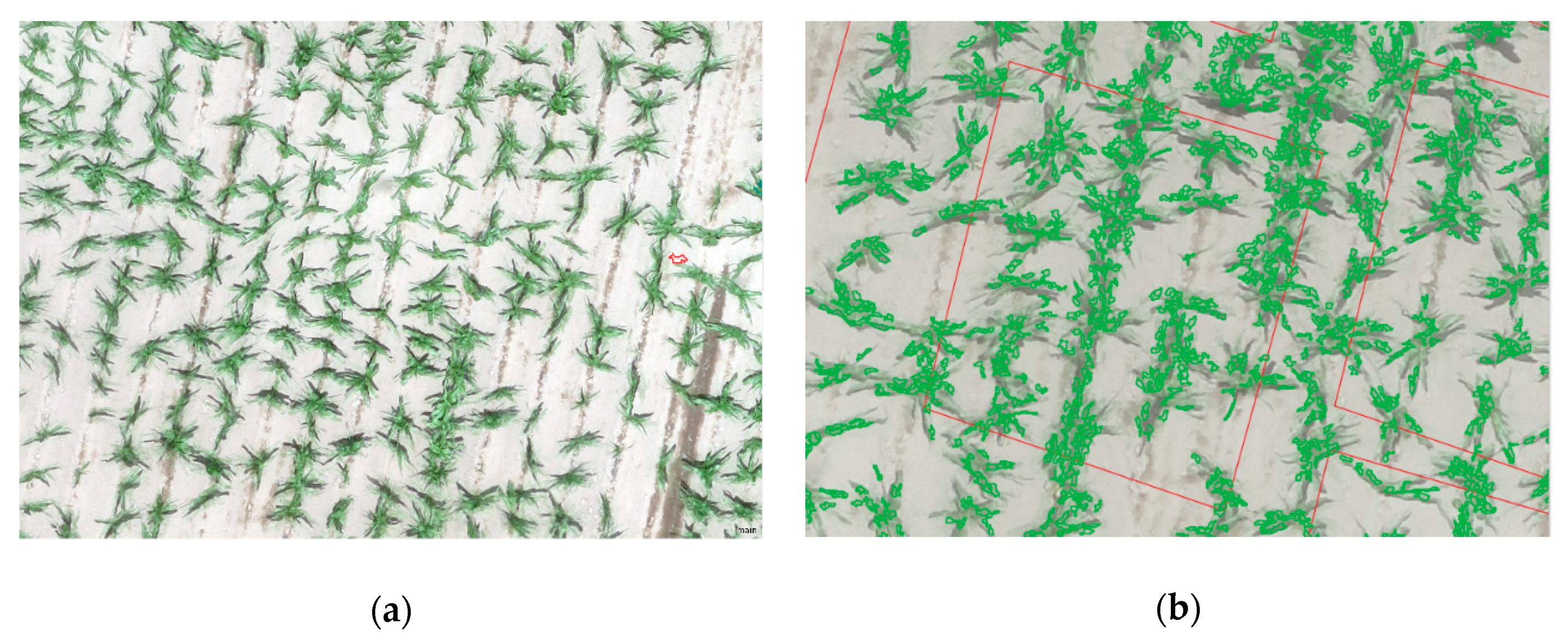
2.3. Plant Count, Determination of Plant Density, and Estimation of Canopy Cover

The corn plants present in the study area were counted digitally according to García et al. [54]. The orthomosaics were transformed from the RGB color model to the CIELab model, where we only worked on the channel a* to extract the vegetation. Corn plant samples were selected at 47 days after planting, twelve of them for each experimental area. Through normalized cross-correlation with the normxcorr2 command in Matlab (Mathworks, Natick, MA, USA), the corn plants present in the binary image were classified and, using an image component labeling technique, assigning a label (1 ... i), the pixels of each plant were grouped. The area of the plants selected in the correlation was used as a criterion, counting plants with 20% less than the minimum area of the smallest selected sample. The digitally counted plants were registered in a table. The plant density (plants m⁻²) in each experimental area was calculated according to the following:

$$\mathrm{Pd}=\frac{\mathrm{Np}}{\mathrm{Ea}},$$

(6)

where Pd is the plant density in plants/m², Np is the number of plants present in the sampled area, and Ea is the sampled area in square meters.

The canopy cover was calculated from the generated TGI vegetation index, using the Open Source program licensed under the GNU—General Public License of the Geographic Information System (QGIS) and System for Automated Geoscientific Analyses (SAGA) [55]. In QGIS, the K-Means Clustering for Grids module was used to group the pixels into two classes: soil and vegetation, through the combined method of minimum distance and simple scaling [56]. The K-means method of image segmentation is a technique that does not use the histogram for the segmentation process, so it is not affected by the noise introduced in the image, evaluating and grouping the different pixels in similar data sets, being suitable for large data sets. On the other hand, the K-means approach in image segmentation is fast and efficient in terms of computational cost [57,58]. In the classification of pixels into two classes in QGIS, a binary raster was generated, where pixels with a value of 0 belong to soil and pixels with a value of 1 belong to vegetation, or vice versa. Thus, the estimation of the percentage of canopy cover was obtained by the following:

$$\mathrm{Cc}=\frac{\mathrm{NP}}{\mathrm{TP}}$$

(7)

where Cc is the canopy cover, NP are the pixels corresponding to vegetation per unit area, and TP is the total pixels per unit area.

Sampling was carried out in four 11 m² polygons for each replicate, according to Figure 1a. In each of them, the canopy cover (Figure 1b,c) and the plant density for the two flight dates were calculated.

2.4. Vegetation Pixels’ Segmentation and Extraction of the Indices Values

The images acquired through the sensors and the orthomosaics generated from them contain reflectance corresponding to soil and vegetation, but only the reflectance corresponding to vegetation was of interest to us. With the eCognition software and the object-based image analysis (OBIA) technique, multi-resolution segmentation was realized. This combines pixels or adjoining objects present in the image based on spectral and shape criteria. It also works according to the scale of the objects present; large scale results in large objects, and vice versa [59]. The homogeneity criterion measures how homogeneous or heterogeneous the object present in the image is, calculated from a combination of object color and shape properties. Color homogeneity is based on the standard deviation of the spectral colors. Shape homogeneity is based on the deviation of a compact (or smooth) shape and can have a value of up to 0.9. In the segmentation process, a 10-scale value was used and the homogeneity criteria like shape and compactness were 0.1 and 0.5, respectively. For the classification of the segmented pixels in the image, three classes present in the image (Figure 2a,b) were determined: soil, vegetation, and shadows. Supervised classification of the nearest neighbor was used to select pixel samples for each class; they were compared with the other objects present with respect to the mean and standard deviation of the supervised sample [60].

Once the pixels present in the image were classified, we exported the pixels classified in the corn class (Figure 3a,b) as polygons in shape file format, with the QGIS software. The mean values of the indices calculated for each polygon of corn class were extracted through the zone statistics complement; the values were stored in a shape file. The mean values obtained from the indices were extracted for 76 sampled polygons, 4 per replicate of the 5 treatments as the average of the mean values of all the pixels classified as corn contained in each polygon. The sample polygon of each replicate on the edge of the crop was discarded to eliminate edge effects.

2.5. Development and Training of the Feed-Forward Neural Network

A multilayer perceptron type feed-forward neural network was developed using Matlab software (Mathworks, Natick, MA, USA). A feed-forward neural network contains multiple neurons arranged in layers: input, hidden, and output. The information goes in one direction, so there are no cycles or loops [61]. The input layer receives values of the input variables (x1, x2, ..., xn); between the input layer and the hidden layer are the weights (w1, w2, ..., wn) that represent the memory of the network; and the output neurons return the output (y1, y2, .., yn) through the sum of all the inputs multiplied by the weights plus a value associated with the neuron, called bias (b) [62].

$$\mathrm{y}={\displaystyle {\sum }_{\mathrm{i}=0}^{\mathrm{i}=\mathrm{n}}}{\mathrm{W}}_{\mathrm{i}}{\mathrm{X}}_{\mathrm{i}}+\mathrm{b},$$

(8)

The outputs of the neurons before passing to the other nodes are transformed through an activation function f(x) to limit the output of the neuron. The precision in the prediction by a neural network is related to the type of activation function used; the non-linear activation functions are the most used (Sigmoid, Hyperbolic Tangent, Rectified liner Unit (ReLU), Exponential Linear Unit (ELU), Softmax) [63,64], so the final output (a) will be as follows:

$$\mathrm{a}=\mathrm{f}\left({\displaystyle {\sum }_{\mathrm{i}=0}^{\mathrm{i}=\mathrm{n}}}{\mathrm{W}}_{\mathrm{i}}{\mathrm{X}}_{\mathrm{i}}+\mathrm{b}\right),$$

(9)

As input parameters or variables, we used the mean value of the vegetation indices, the canopy cover, and the plant density, as well as the yield in tons per hectare as labels and output parameters. In total, 70% of the total data entered into the neural network was used for training, 15% for validation, and 15% for testing using a random partition of the entire data set. For each combination of input variables, the neural network was trained ten times using ten different random data sets. The training algorithm used was Levenberg–Marquart [65,66], which is a training function that updates the values in the weights and bias according to the Levenber–Marquart optimization. Tan-sigmoid was used as activation function, as it defines the behavior of the neurons in charge of calculating the degree or state of activation of the neuron, according to the total input function [67]. The descending gradient with momentum type was used as a learning rule, as it calculates the change in weight (W) for a given neuron. On the basis of the weights of the input neurons and the error (E), the weight W, the learning rate (LR), and the moment constant (MC) are calculated, according to the descent of the gradient with momentum. The objective of training the neural network is to minimize the resulting errors for a training data set by adjusting the weights (W).

2.6. Statistical Analysis

For the performance analysis of the estimated yields by the neural network, estimated yields were compared to the observed yields, estimating the root mean square error (RMSE), the mean absolute error (MAE), and the correlation coefficient (R) in the training, validation, testing, and total data entered into the neural network. The correlation coefficient between the observed yields and the vegetation indices, the plant density, and the canopy cover was also estimated.

$${\mathrm{E}}_{\mathrm{s}}=\left(\mathrm{EY}-\mathrm{OY}\right),$$

(10)

$$\mathrm{MAE}=\frac{1}{\mathrm{N}}{\displaystyle {\sum }_{\mathrm{i}=1}^{\mathrm{N}}}\left|{\left({\mathrm{E}}_{\mathrm{s}}\right)}_{\mathrm{i}}\right|,$$

(11)

$$\mathrm{RMSE}=\sqrt{\frac{{\sum }_{\mathrm{i}=1}^{\mathrm{N}}{\left(\mathrm{EY}-\mathrm{OY}\right)}^2}{\mathrm{N}}},$$

(12)

where N is the number of the sampled polygon, $\left|{\left({\mathrm{E}}_{\mathrm{s}}\right)}_{\mathrm{i}}\right|$ is the absolute value of E_s, EY is the estimated yield, and OY is the observed yield.

2.7. Variables’ Relative Importance in the Yield Estimation Using Garson’s Algorithm

Neural network models are difficult to interpret and it is difficult to identify which predictors are the most important and how they relate to the property being modeled. The weights connecting neurons in a neural network are partially analogous to the coefficients in a generalized linear model, and these weights combined with their effects on model predictions represent the relative importance of predictors in their associations with the variable being predicted [68]. Garson’s algorithm discriminates the relative importance of the predictor variables for a single response variable, that is, the force with which a specific variable explains the predicted variable is determined by identifying all the weighted connections between the nodes of interest, and identifying the weights that connect to the specific input node that passes through the neural network and reaches the variable that is being predicted. This allows to obtain a unique value for each descriptor variable used in the neural network model [69,70]. To know the predictor variables’ relative importance (NDVI, NDRE, WDRVI, EXG, TGI, VARI, canopy cover, and density) in the corn yield estimation, Garson’s algorithm was used.

3. Results and Discussion

3.1. Corn Plant Vegetation Indices

The segmentation and classification of objects into soil and vegetation allowed to filter mean values of the vegetation indices with respect to the pixels belonging to corn plants.

Table 3. Mean values of the vegetation indices and yield for each replicate of the treatments under different degrees of nitrogen fertilization.

DAS	Treatment	Vegetation Index
		NDVI		NDRE		WDRVI		EXG		TGI		VARI		Yield (g plant−1)
		Mean	Std DeV	Mean	Std DeV	Mean	Std DeV	Mean	Std DeV	Mean	Std DeV	Mean	Std DeV	Mean	Std DeV
47	N140	0.46	0.05	0.19	0.02	−0.55	0.04	0.40	0.03	0.40	0.03	0.12	0.02	109.3	19.6
	N200	0.48	0.04	0.19	0.01	−0.53	0.04	0.42	0.03	0.42	0.03	0.13	0.02	134.0	2.7
	N260	0.46	0.05	0.18	0.02	−0.55	0.05	0.41	0.02	0.41	0.02	0.13	0.02	135.6	2.7
	N320	0.46	0.04	0.18	0.01	−0.55	0.04	0.42	0.04	0.42	0.04	0.13	0.02	137.1	3.6
	N380	0.47	0.05	0.19	0.02	−0.53	0.05	0.43	0.02	0.43	0.03	0.14	0.01	138.3	5.3
79	N140	0.90	0.02	0.26	0.02	−0.13	0.06	0.53	0.03	0.54	0.01	0.13	0.02	109.3	19.6
	N200	0.91	0.01	0.26	0.03	−0.10	0.06	0.54	0.03	0.54	0.01	0.14	0.02	134.0	2.7
	N260	0.90	0.01	0.25	0.02	−0.13	0.06	0.52	0.03	0.54	0.01	0.13	0.02	135.6	2.7
	N320	0.90	0.01	0.25	0.02	−0.12	0.05	0.53	0.04	0.54	0.01	0.13	0.02	137.1	3.6
	N380	0.90	0.01	0.25	0.02	−0.11	0.05	0.53	0.03	0.54	0.01	0.13	0.02	138.3	5.3

shows the mean values computed through segmentation and classification of the objects present in the image for two dates in the corn crop development. Differences are observed in the mean values of the vegetation indices for 47 and 79 days after sowing. The classification of the pixels captured in the sensors into two classes allowed us to extract the values of the indices belonging to corn, so the result was a mean value of the vegetation. Contrarily, if the classification of the pixels into classes was not carried out, there would be a bias when considering pixels belonging to soil and shadows in the mean computation for the polygons taken as a sample, resulting in a mixed value of corn plants and soil pixels. Vegetation indices values increased for 79 DAS with respect to the values shown for 47 DAS, except for the VARI index, which did not present a wide variation with the crop development. Similar results were shown in the studies carried out by Gitelson et al. [53,71]. Vegetation indices did not show differences for the nitrogen treatments used; similar results are reported by Olson et al. [19].

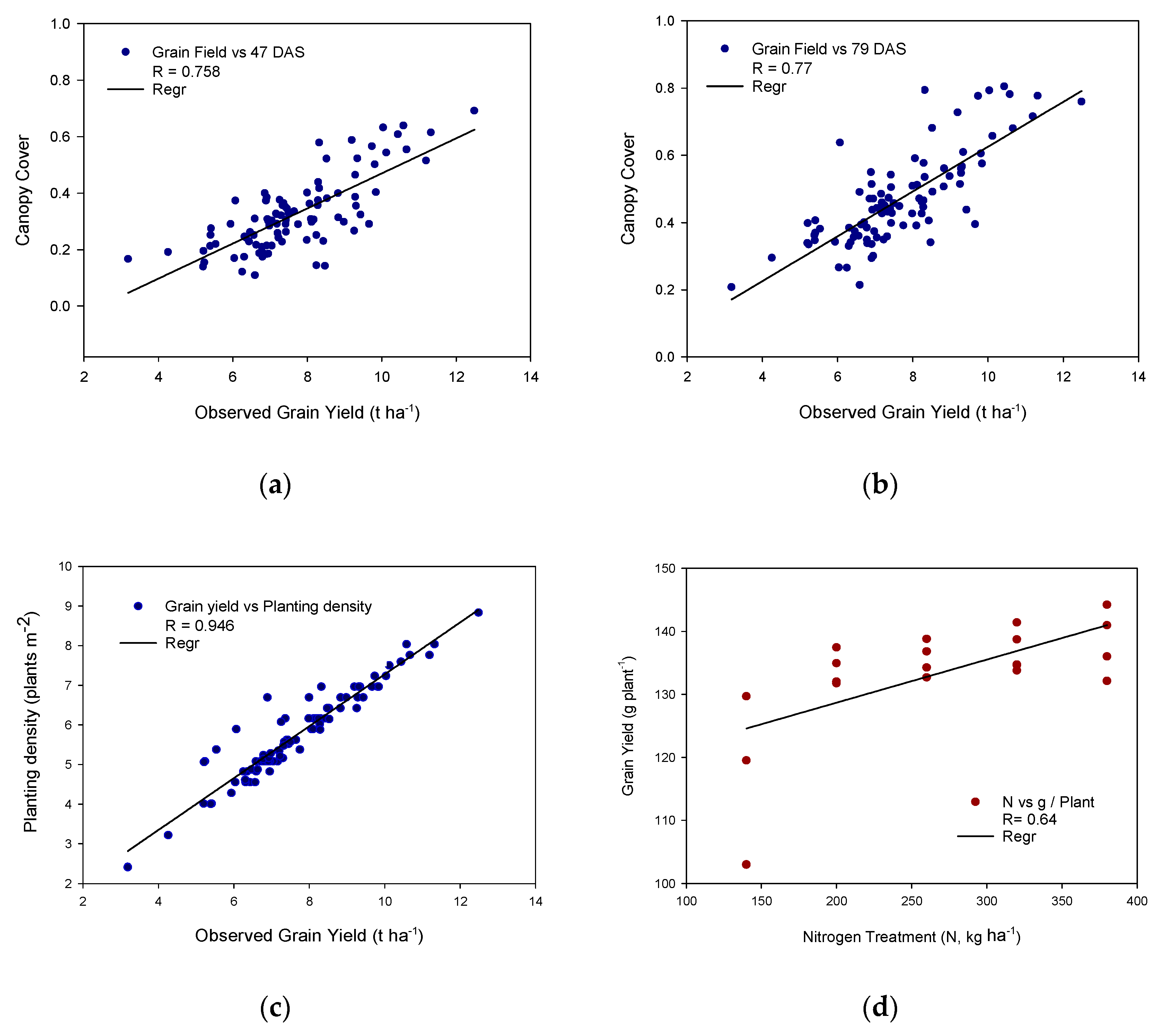
3.2. Plant Density, Canopy Cover, and Yield

Figure 4 shows the correlation coefficient at 47 and 79 days after sowing between the canopy cover, plant density, and yield; it also shows the correlation coefficient between the applied nitrogen dose and grain yield per plant. The canopy cover calculated through the TGI index is closely related to the density and grain yield of corn; the higher the density, the higher the cover and yield for 47 and 79 DAS. Therefore, corn yield has a direct response to canopy cover and planting density. For the period from 47 to 79 DAS, the canopy cover increased by an average of 15% with a standard deviation of 5%. The correlation coefficient for canopy cover was similar for both flight dates, around 0.76. Plant density, according to Figure 4c, showed a high correlation with a coefficient of 0.94; thus, at a higher density, an increase in grain yield is expected. This means that plant density explained 94% of the yield. Positive yield responses have been reported with an increase in planting density, a significant increase of 4.5–6, moderate of 6–7.5, and low of 7.5 to 9 plants per square meter [14]. The different nitrogen treatments applied to the experiment influenced grain yield per plant; as the nitrogen dose increases, there is a positive gain in grain yield per plant, as observed in Figure 4d, with mean grain weight yield per plant of 109.3, 134.0, 135.6, 137.1, and 138.3 g per plant for 140, 200, 260, 320, and 380 kg ha⁻¹, for the conditions of the experimental site and the variety used.

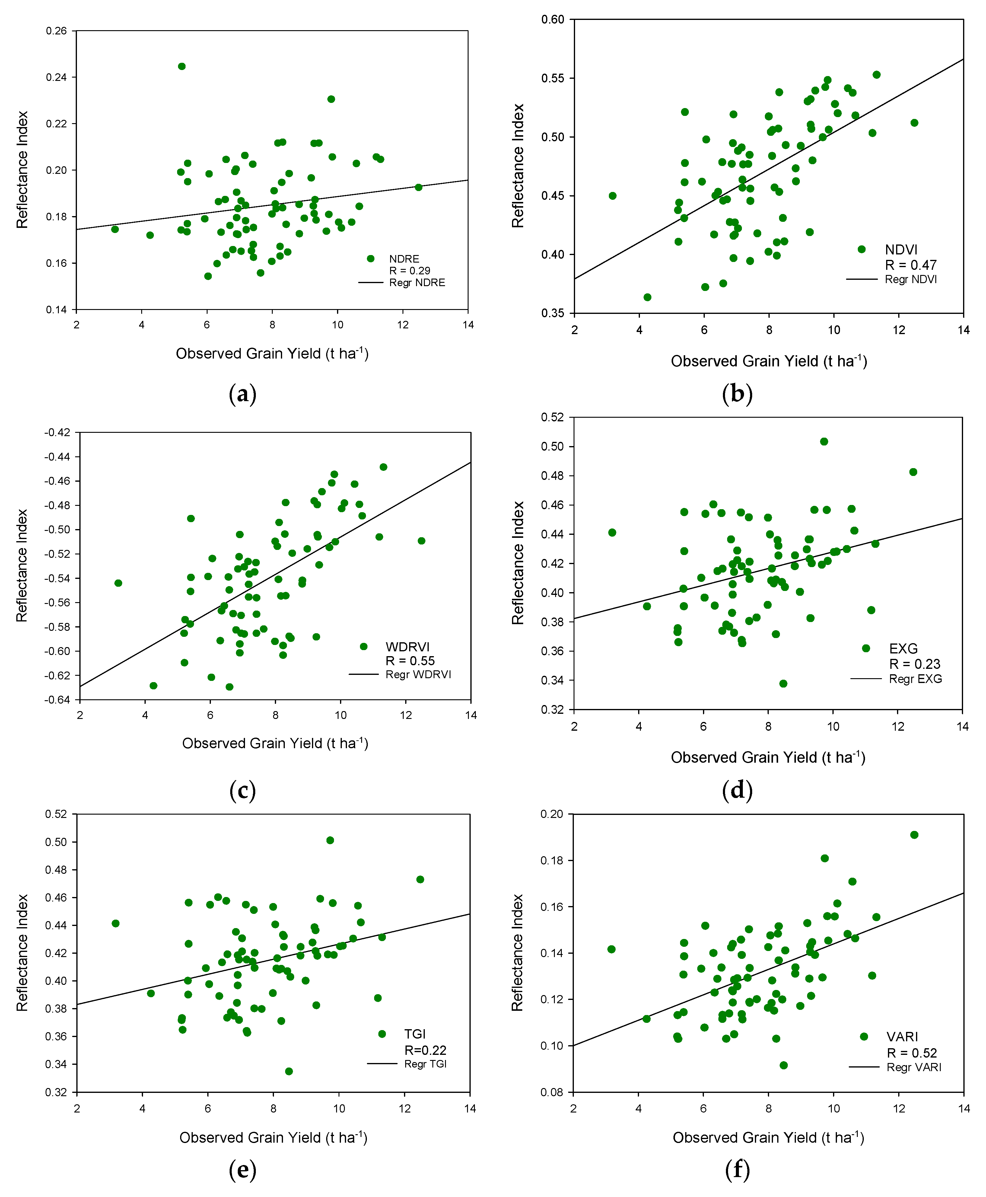
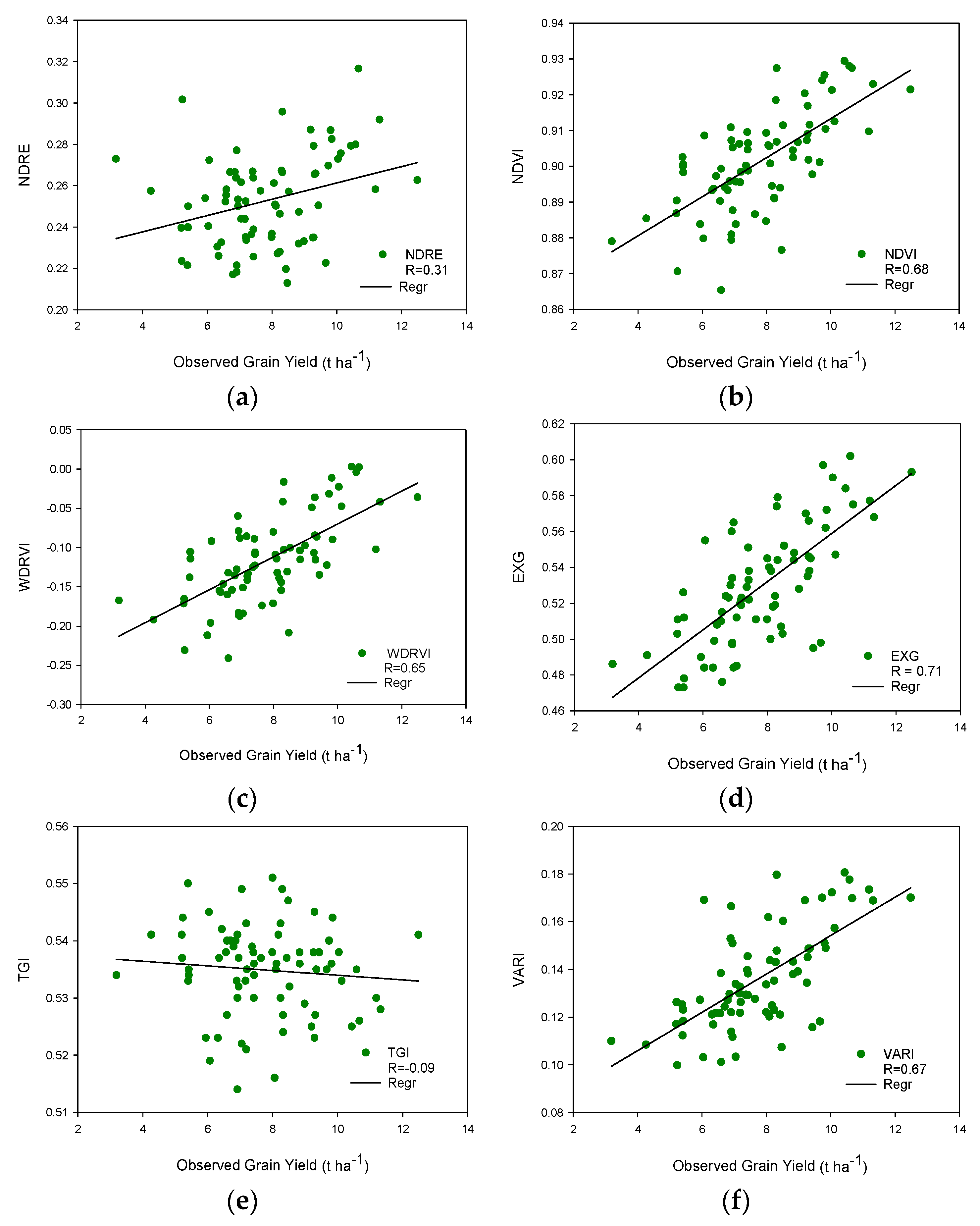
3.3. Vegetation Indices and Yield

For flights at 47 DAS and 79 DAS, six vegetation indices (NDVI, NDRE, WDRVI, EXG, TGI, VARI) were generated; three multispectral indices and three indices in the visible spectrum (RGB). Figure 5 shows the correlation coefficient between the vegetation indices corresponding to the corn class and the observed grain yield at 47 DAS. During the 47 DAS, the WDRVI index presented values ranging from −0.45 to −0.63 with a correlation coefficient of 0.54, thus presenting the highest correlation at this crop stage. Meanwhile, the NDRE index showed a low correlation of 0.23 with values ranging from 0.15 to 0.24. The NDVI ranged from 0.36 to 0.55. In the study carried out by Maresma et al. [72], they found that the WDRVI better explained the corn grain yield with different nitrogen treatments; on the other hand, the index is reported to be sensitive to the leaf area index (LAI) and the canopy cover [53].

At 72 DAS, the correlation coefficient of the vegetation indices with respect to the observed corn grain yield increases slightly for all the indices, which is related to the increase in canopy cover and the presence of more pixels in the corn class and fewer pixels in the soil category. In Figure 6, the NDVI, NDRE, and WDRVI showed correlation coefficients of 0.68, 0.31, and 0.65, respectively, and the indices values resulted in ranges of 0.86–0.92, 0.21–0.31, and −0.241 to 0.003, respectively. These increases in the vegetation indices are related to the increase in biomass, leaf area index (LAI), leaf chlorophyll content (LCC), canopy cover (CC), and yield [23,50,72,73,74]. The NDVI can explain 0.68 of the corn grain yield. Figure 6 shows a proportional relation between an increase in grain yield and an increase in the NDVI index; the same is true for the NDRE and WDRVI. Regarding the normalized EXG, TGI, and VARI indices computed in the visible spectrum (RGB) for 47 DAS, Figure 5d,e show that EXG and TGI presented low correlation coefficients, 0.22 and 0.23, respectively. The VARI in Figure 5f showed a better fit regarding to these indices, with a correlation coefficient of 0.52. In Figure 6, the values of the indices were found between 0.338–0.503, 0.335–0.501, and 0.02–0.19 for EXG, TGI, and VARI, respectively, according to the sampled polygons. In Figure 6 at 79 DAS, 0.71 of the yield can be explained by the EXG index, while VARI showed a value of 0.67. TGI showed a low correlation coefficient. The values of the indices ranged as follows: 0.47–0.60, 0.51–0.55, and 0.10–0.18 for EXG, TGI, and VARI, respectively. Some research works indicate that the VARI has a high correlation with grain yield, chlorophyll content, and the fraction of photosynthetically active radiation intercepted [75,76].

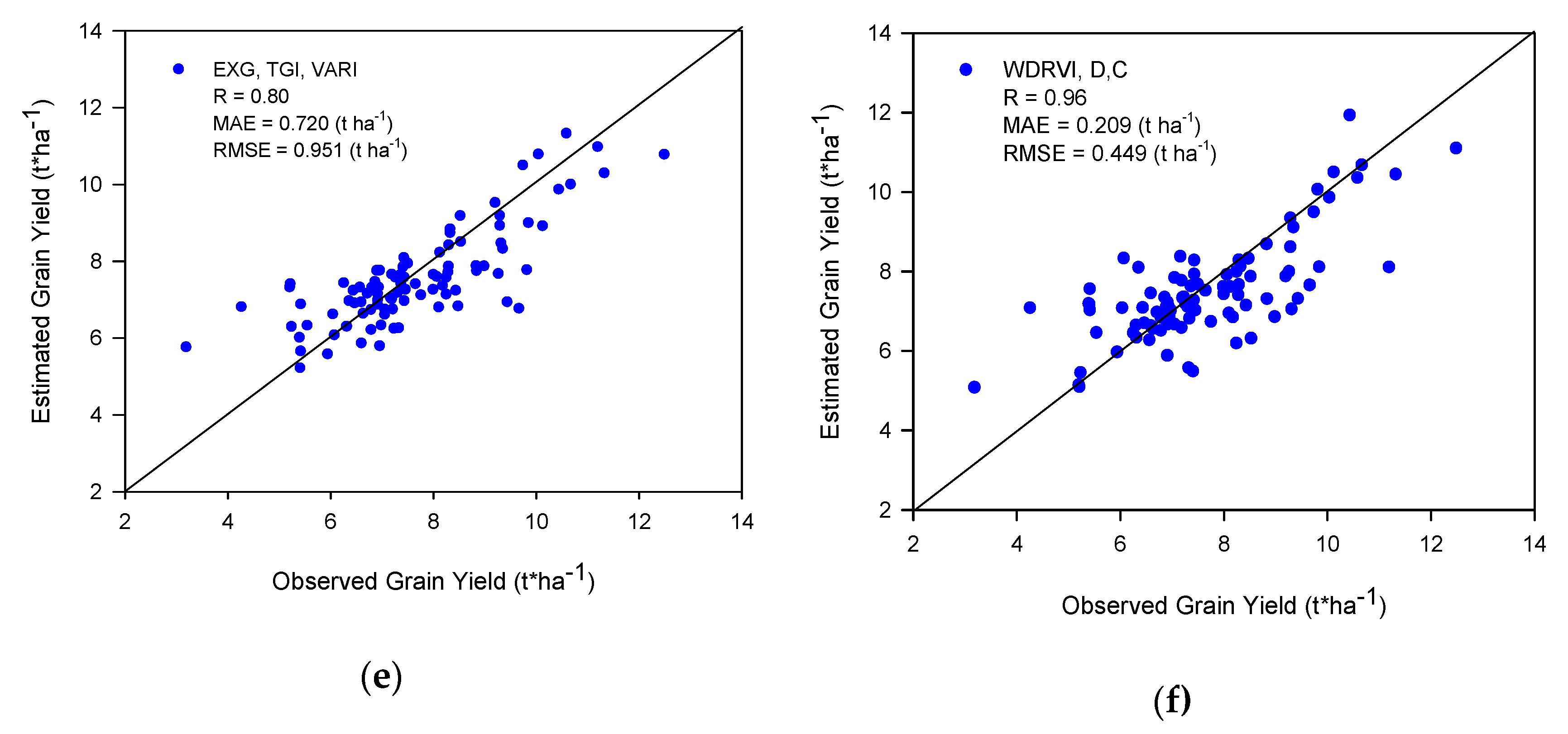
3.4. Training, Validation, and Testing of the Artificial Neural Network for Estimating Yield

A feed-forward neural network was created with 2 layers and 40 neurons, where a combination of the normalized vegetation indices, plant density, and canopy cover, according to

Table 4. Training, validation, and testing of the artificial neural network with different input variables from vegetation indices, plant density, and canopy cover for the estimation of corn grain yield at 47 and 79 days after sowing (DAS).

Input Variables	47 DAS						79 DAS
	R Training	R Validation	R Test	R Total	MAE (t ha−1)	RMSE (t ha−1)	R Training	R Validation	R Test	R Total	MAE (t ha−1)	RMSE (t ha−1)
NDVI, NDRE, WDRVI, D, C	0.96	0.97	0.98	0.97	0.285	0.414	0.96	0.97	0.98	0.96	0.242	0.337
NDVI, NDRE, WDRVI, TGI, EXG, VARI, D, C	0.98	0.93	0.98	0.97	0.307	0.400	0.97	0.90	0.99	0.97	0.249	0.425
NDRE, D, C	0.97	0.99	0.95	0.97	0.256	0.365	0.97	0.88	0.97	0.96	0.278	0.437
EXG, D, C	0.97	0.98	0.99	0.98	0.252	0.354	0.95	0.97	0.99	0.96	0.280	0.431
TGI, EXG, VARI, D, C	0.97	0.94	0.96	0.96	0.331	0.470	0.92	0.97	0.96	0.94	0.292	0.562
C, D	0.97	0.93	0.95	0.96	0.298	0.441	0.96	0.92	0.95	0.96	0.298	0.441
NDVI, D, C	0.96	0.99	0.93	0.97	0.280	0.425	0.96	0.94	0.91	0.96	0.300	0.449
TGI, D, C	0.96	0.97	0.98	0.97	0.304	0.414	0.94	0.95	0.97	0.95	0.312	0.459
VARI, D, C	0.97	0.99	0.93	0.97	0.279	0.395	0.97	0.93	0.90	0.95	0.347	0.571
NDVI, NDRE, WDRVI, TGI, EXG, VARI, C	0.92	0.86	0.96	0.92	0.512	0.643	0.94	0.97	0.88	0.94	0.381	0.538
NDVI, NDRE, WDRVI, TGI, EXG, VARI	0.80	0.94	0.92	0.86	0.622	0.809	0.84	0.91	0.90	0.86	0.528	0.876
EXG, C	0.81	0.81	0.84	0.81	0.733	0.938	0.80	0.81	0.84	0.80	0.623	0.947
NDVI, NDRE, WDRVI	0.74	0.65	0.85	0.73	0.811	1.093	0.82	0.85	0.87	0.85	0.641	0.837
NDVI, C	0.83	0.82	0.90	0.84	0.597	0.883	0.80	0.86	0.88	0.82	0.649	0.884
VARI, C	0.86	0.94	0.51	0.85	0.604	0.836	0.86	0.79	0.92	0.86	0.653	0.917
NDVI, NDRE, WDRVI, C	0.81	0.93	0.83	0.84	0.618	0.874	0.87	0.87	0.62	0.84	0.672	0.856
WDRVI, C	0.87	0.62	0.95	0.87	0.584	0.784	0.82	0.64	0.56	0.79	0.689	0.971
TGI, EXG, VARI	0.69	0.64	0.82	0.67	0.908	1.189	0.83	0.72	0.72	0.80	0.720	0.951
TGI, EXG, VARI, C	0.86	0.90	0.87	0.86	0.629	0.817	0.78	0.93	0.71	0.78	0.746	1.015
WDRVI, D, C	0.99	0.99	0.99	0.99	0.028	0.125	0.96	0.99	0.89	0.96	0.209	0.449
NDRE, C	0.75	0.98	0.97	0.81	0.527	0.986	0.68	0.68	0.55	0.65	0.774	1.179
TGI, C	0.85	0.62	0.78	0.82	0.701	0.909	0.50	0.62	0.29	0.54	1.017	1.380

NDVI, normalized difference vegetation index; NDRE, normalized difference red edge index; WDRVI, wide dynamic range vegetation index; EXG, green extraction index; TGI, triangular greenness index; VARI, visible atmospherically resistant index; C, canopy cover; D, plant density (plants * m⁻²); MAE, mean absolute error; RMSE, root mean square error.

for 47 DAS, was entered as input parameters. Another neural network for 79 DAS was created to estimate the corn grain yield of 76 sampled polygons obtained from all of the experimental treatments. The results are shown in Table 4; in column one, we have the combination of input parameters: NDVI, NDRE, WDRVI, EXG, TGI, VARI, canopy cover (C), and plant density (D). The correlation coefficient for training, validation, testing, and total entered data is also presented, as well as the mean absolute error (MAE) and the root mean square error (RMSE).

For 47 DAS, which is shown in Table 4 and Figure 7, the input parameters WDRVI, plant density, and canopy cover showed the highest correlation coefficient and the smallest errors for the corn grain yield estimation (R = 0.99, MAE = 0.028 t ha⁻¹, RMSE = 0.125 t ha⁻¹) when the total data were used. Using the same parameters above, except plant density as input parameter in the neural network, the correlation coefficient decreased, and the errors increased (R = 0.87, MAE = 0.584 t ha⁻¹, RMSE = 0.784 t ha⁻¹), which indicates that plant density is an important parameter in estimating yield for this flight date. A combination of six vegetation indices (NDVI, NDRE, WDRVI, EXG, TGI, VARI), plant density, and canopy cover generates a model with high correlation in yield estimation (R = 0.97), with a mean absolute error of 307 kg per hectare and a root mean square error of 400 kg per hectare. Doing the same analysis, but without plant density, a lower correlation was obtained with the total data (R = 0.92, MAE = 0.512 t ha⁻¹ y RMSE = 0.643 t ha⁻¹), having greater precision than the combination of WDRVI and canopy cover. On the other hand, a combination of only six vegetation indices as input parameters resulted in a correlation of 0.86 and an MAE of 0.622 t ha⁻¹, with an RMSE of 0.809 t ha⁻¹ when using the total data in yield estimation. This is good if we consider that there is a decrease in computational cost in obtaining plant density and canopy cover. The EXG index, canopy cover, and plant density showed a correlation coefficient of 0.98. In general, combinations that include canopy cover presented high correlation coefficients (R ≥ 0.80), and incorporating plant density as an input parameter increased the value of the correlation coefficient (R ≥ 0.95). The multispectral indices without canopy cover and plant density as input parameters showed a good correlation (R = 0.73, MAE = 0.811 t ha⁻¹, RMSE = 1.093 t ha⁻¹) in yield estimation. The RGB indices without canopy cover and plant density showed a lower correlation than the multispectral indices, explaining 0.67 of the corn grain yield. Plant density and canopy cover showed a high correlation (R = 0.96, MAE = 0.298 t ha⁻¹, RMSE = 0.441 t ha⁻¹).

For 79 DAS, which is shown in Figure 8 and Table 4, the six vegetation indices, canopy cover, and plant density presented the highest correlation coefficient and the smallest errors (R = 0.97, MAE = 0.249 t ha⁻¹, RMSE = 0.425 t ha⁻¹) when the total data were used. The EXG index, canopy cover, and plant density also showed a good correlation coefficient and small errors (R = 0.97, MAE = 0.280 t ha⁻¹, RMSE = 0.431 t ha⁻¹) in yield estimation. Vegetation indices and canopy cover increased the correlation coefficient with respect to 47 DAS, while the indices without canopy cover and plant density maintained a similar correlation coefficient for all the data. The TGI index and canopy cover showed the lowest correlation and biggest errors (R = 0.54, MAE = 1.017 t ha⁻¹, RMSE = 1.380 t ha⁻¹) in the yield estimate. The multispectral vegetation indices and the visible vegetation indices presented a high correlation in the estimation of corn grain yield at 47 and 79 DAS for the different nitrogen doses tested, presenting slightly higher correlations at 47 DAS.

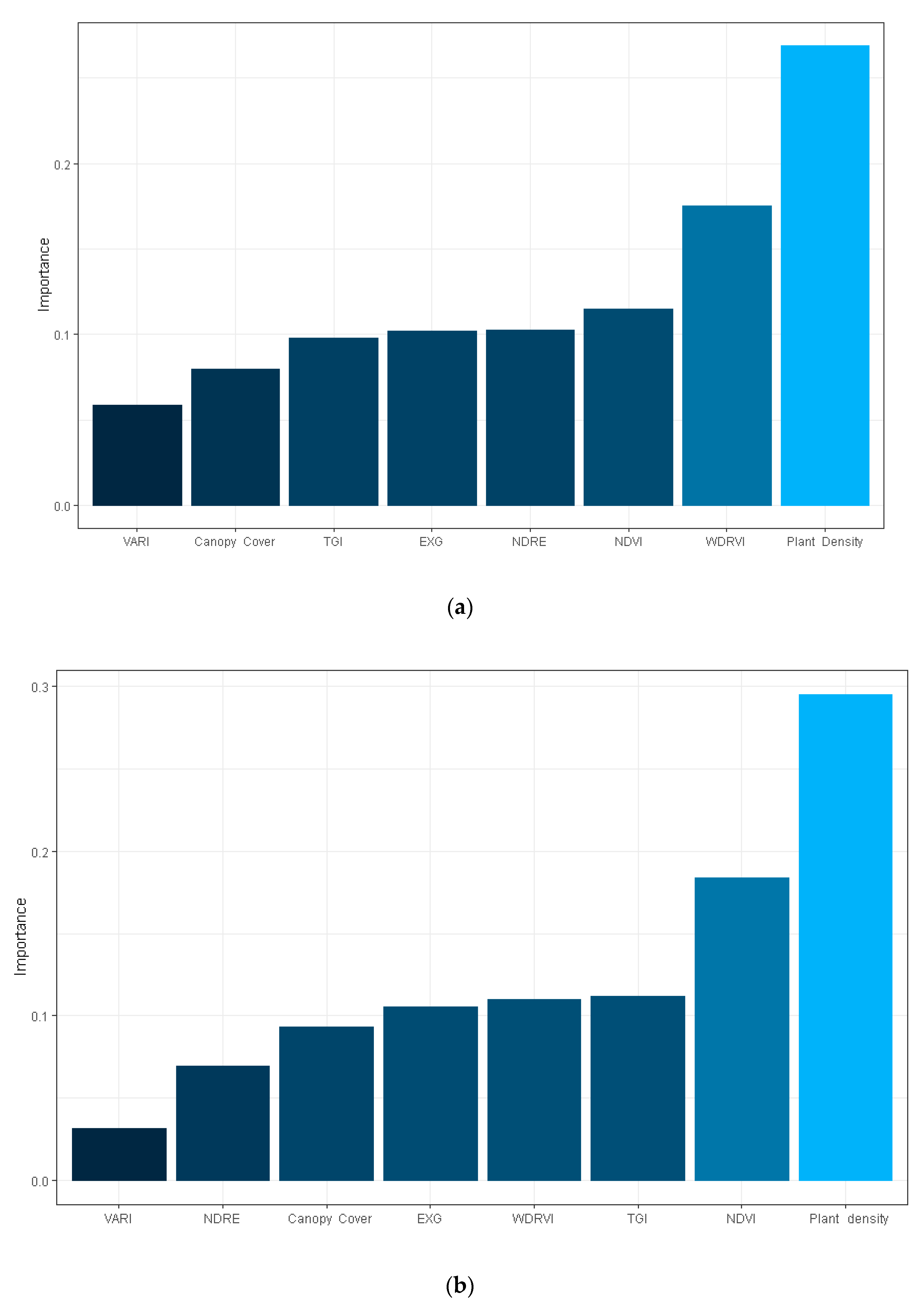
3.5. Variables’ Relative Importance in the Yield Estimation Using Garson’s Algorithm

The importance of the predictor variables (NDVI, NDRE, WDRVI, EXG, TGI, VARI, density, and canopy cover) with respect to the predicted variable (yield) is shown in Figure 9; this was calculated using Garson’s algorithm. The results show that the density is the most important predictor for the 47 and 79 DAS with a relative importance of 0.269 and 0.295, respectively; the WDRVI index (0.175) was the second best predictor in importance for the 47 DAS; while the NDVI index (0.184) for the 79 DAS. The VARI index was the least important predictor in the yield estimation for the 47 and 79 DAS with 0.058 and 0.031 relative importance, respectively.

4. Conclusions

In the present study, the corn grain yield was estimated designing a neural network model based on vegetation indices, canopy cover, and plant density. The relative importance of the predictor variables was also analyzed. The information obtained through the digital processing of images taken by unmanned aerial vehicles allowed to monitor the crop development. The correlation coefficient between the plant density, obtained through the digital count of corn plants, and the corn grain yield was 0.94; this variable was the one with the highest relative importance in the yield estimation according to Garson’s algorithm. The canopy cover, digitally estimated by object-oriented classification and using the TGI index, showed a correlation coefficient of 0.77 with respect to the corn grain yield, while the relative importance of this variable in the yield estimation was 0.080 and 0.093 for the 47 and 79 DAS, respectively. The WDRVI, plant density, and canopy cover showed the highest correlation coefficient and the smallest errors (R = 0.99, MAE = 0.028 t ha⁻¹, RMSE = 0.125 t ha⁻¹) in the corn grain yield estimation at 47 DAS, with the WDRVI and the density being the variables with the highest relative importance for this crop development date. For the 79 DAS flight, the combination of the NDVI, NDRE, WDRVI, EXG, TGI, and VARI indices, as well as plant density and canopy cover, generated the highest correlation coefficient and the smallest errors (R = 0.97, MAE = 0.249 t ha⁻¹, RMSE = 0.425 t ha⁻¹) in the corn grain yield estimation, with the density and the NDVI being the variables with the highest relative importance with values of 0.295 and 0.184, respectively. However, the WDRVI, plant density, and canopy cover estimated the corn grain yield with acceptable precision (R = 0.96, MAE = 0.209 t ha⁻¹, RMSE = 0.449 t ha⁻¹). The generated neural network models provided a high correlation coefficient between the estimated and the observed corn grain yield; it also showed acceptable errors in the yield estimation. The spectral information registered through remote sensors mounted on unmanned aerial vehicles and its processing in vegetation indices, canopy cover, and plant density allow the characterization and estimation of corn grain yield. Such information is very useful for decision-making and agricultural activities planning.

At the time of establishing agricultural crops, different techniques, tools, and management are used during the crop development, so it is desirable to carry out future trials for different climates, soils, management, and varieties to have a broader database and with greater parameters to be used in the modeling of crop yields through the use of neural networks.

References

1. USDA-Office of the Chief Economist. Available online: https://www.usda.gov/oce/commodity/wasde/ (accessed on 28 April 2020).
2. ASERCA. CIMA. Available online: https://www.cima.aserca.gob.mx/ (accessed on 4 March 2020).
3. Domínguez Mercado, C.A.; de Jesús Brambila Paz, J.; Carballo Carballo, A.; Quero Carrillo, A.R. Red de valor para maíz con alta calidad de proteína. Rev. Mex. Cienc. Agríc. 2014, 5, 391–403. [Google Scholar]
4. Mercer, K.L.; Perales, H.R.; Wainwright, J.D. Climate change and the transgenic adaptation strategy: Smallholder livelihoods, climate justice, and maize landraces in Mexico. Glob. Environ. Chang. 2012, 22, 495–504. [Google Scholar] [CrossRef]
5. Tarancón, M.; Díaz-Ambrona, C.H.; Trueba, I. Cómo alimentar a 9.000 millones de personas en el 2050? In Proceedings of the XV Congreso Internacional de Ingeniería de Proyectos, Huesca, Spain, 6–8 July 2011. [Google Scholar]
6. Cervantes, R.A.; Angulo, G.V.; Tavizón, E.F.; González, J.R. Impactos potenciales del cambio climático en la producción de maíz Potential impacts of climate change on maize production. Investigación Ciencia 2014, 22, 48–53. [Google Scholar]
7. Moore, F.C.; Lobell, D.B. Reply to Gonsamo and Chen: Yield findings independent of cause of climate trends. Proc. Natl. Acad. Sci. USA 2015, 112, E2267. [Google Scholar] [CrossRef] [PubMed] [Green Version]
8. Ruiz Corral, J.A.; Medina García, G.; Ramírez Díaz, J.L.; Flores López, H.E.; Ramírez Ojeda, G.; Manríquez Olmos, J.D.; Zarazúa Villaseñor, P.; González Eguiarte, D.R.; Díaz Padilla, G.; Mora Orozco, C.D.L. Cambio climático y sus implicaciones en cinco zonas productoras de maíz en México. Rev. Mex. Cienc. Agríc. 2011, 2, 309–323. [Google Scholar]
9. Tinoco-Rueda, J.A.; Gómez-Díaz, J.D.; Monterroso-Rivas, A.I.; Tinoco-Rueda, J.A.; Gómez-Díaz, J.D.; Monterroso-Rivas, A.I. Efectos del cambio climático en la distribución potencial del maíz en el estado de Jalisco, México. Terra Latinoam. 2011, 29, 161–168. [Google Scholar]
10. Bolaños, H.O.; Vázquez, M.H.; Juárez, G.G.; González, G.S. Cambio climático: Una percepción de los productores de maíz de temporal en el estado de Tlaxcala, México. CIBA Rev. Iberoam. Las Cienc. Biológicas Agropecu. 2019, 8, 1–26. [Google Scholar] [CrossRef] [Green Version]
11. Khaki, S.; Wang, L.; Archontoulis, S.V. A CNN-RNN Framework for Crop Yield Prediction. Front. Plant Sci. 2020, 10. [Google Scholar] [CrossRef]
12. Dahikar, S.S.; Rode, S.V. Agricultural Crop Yield Prediction Using Artificial Neural Network Approach. Int. J. Innov. Res. Electr. Electron. Instrum. Control Eng. 2014, 2, 683–686. [Google Scholar]
13. Li, A.; Liang, S.; Wang, A.; Qin, J. Estimating Crop Yield from Multi-temporal Satellite Data Using Multivariate Regression and Neural Network Techniques. Photogramm. Eng. Remote Sens. 2007, 73, 1149–1157. [Google Scholar] [CrossRef] [Green Version]
14. Assefa, Y.; Vara Prasad, P.V.; Carter, P.; Hinds, M.; Bhalla, G.; Schon, R.; Jeschke, M.; Paszkiewicz, S.; Ciampitti, I.A. Yield Responses to Planting Density for US Modern Corn Hybrids: A Synthesis-Analysis. Crop. Sci. 2016, 56, 2802–2817. [Google Scholar] [CrossRef]
15. Kitano, B.T.; Mendes, C.C.T.; Geus, A.R.; Oliveira, H.C.; Souza, J.R. Corn Plant Counting Using Deep Learning and UAV Images. IEEE Geosci. Remote Sens. Lett. 2019, 1–5. [Google Scholar] [CrossRef]
16. Lindblom, J.; Lundström, C.; Ljung, M.; Jonsson, A. Promoting sustainable intensification in precision agriculture: Review of decision support systems development and strategies. Precis. Agric. 2017, 18, 309–331. [Google Scholar] [CrossRef] [Green Version]
17. Geipel, J.; Link, J.; Claupein, W. Combined Spectral and Spatial Modeling of Corn Yield Based on Aerial Images and Crop Surface Models Acquired with an Unmanned Aircraft System. Remote Sens. 2014, 6, 10335–10355. [Google Scholar] [CrossRef] [Green Version]
18. Tsouros, D.C.; Bibi, S.; Sarigiannidis, P.G. A Review on UAV-Based Applications for Precision Agriculture. Information 2019, 10, 349. [Google Scholar] [CrossRef] [Green Version]
19. Olson, D.; Chatterjee, A.; Franzen, D.W.; Day, S.S. Relationship of Drone-Based Vegetation Indices with Corn and Sugarbeet Yields. Agron. J. 2019, 111, 2545–2557. [Google Scholar] [CrossRef]
20. Xue, J.; Su, B. Significant Remote Sensing Vegetation Indices: A Review of Developments and Applications. J. Sens. 2017. [Google Scholar] [CrossRef] [Green Version]
21. Peñuelas, J.; Filella, I. Visible and near-infrared reflectance techniques for diagnosing plant physiological status. Trends Plant Sci. 1998, 3, 151–156. [Google Scholar] [CrossRef]
22. Serrano, L.; Filella, I.; Peñuelas, J. Remote Sensing of Biomass and Yield of Winter Wheat under Different Nitrogen Supplies. Crop. Sci. 2000, 40, 723–731. [Google Scholar] [CrossRef] [Green Version]
23. Buchaillot, M.; Gracia-Romero, A.; Vergara-Diaz, O.; Zaman-Allah, M.A.; Tarekegne, A.; Cairns, J.E.; Prasanna, B.M.; Araus, J.L.; Kefauver, S.C. Evaluating Maize Genotype Performance under Low Nitrogen Conditions Using RGB UAV Phenotyping Techniques. Sensors 2019, 19, 1815. [Google Scholar] [CrossRef] [Green Version]
24. Kefauver, S.C.; El-Haddad, G.; Vergara-Diaz, O.; Araus, J.L. RGB picture vegetation indexes for High-Throughput Phenotyping Platforms (HTPPs). In Remote Sensing for Agriculture, Ecosystems, and Hydrology XVII, Volume 9637; International Society for Optics and Photonics: Touluse, France, 2015; p. 96370. [Google Scholar] [CrossRef]
25. Vergara-Diaz, O.; Kefauver, S.C.; Elazab, A.; Nieto-Taladriz, M.T.; Araus, J.L. Grain yield losses in yellow-rusted durum wheat estimated using digital and conventional parameters under field conditions. Crop. J. 2015, 3, 200–210. [Google Scholar] [CrossRef] [Green Version]
26. Jeong, J.H.; Resop, J.P.; Mueller, N.D.; Fleisher, D.H.; Yun, K.; Butler, E.E.; Timlin, D.J.; Shim, K.M.; Gerber, J.S.; Reddy, V.R.; et al. Random Forests for Global and Regional Crop Yield Predictions. PLoS ONE 2016, 11. [Google Scholar] [CrossRef] [PubMed]
27. Oguntunde, P.G.; Lischeid, G.; Dietrich, O. Relationship between rice yield and climate variables in southwest Nigeria using multiple linear regression and support vector machine analysis. Int. J. Biometeorol. 2018, 62, 459–469. [Google Scholar] [CrossRef] [PubMed]
28. Pantazi, X.E.; Moshou, D.; Alexandridis, T.; Whetton, R.L.; Mouazen, A.M. Wheat yield prediction using machine learning and advanced sensing techniques. Comput. Electron. Agric. 2016, 121, 57–65. [Google Scholar] [CrossRef]
29. Panda, S.S.; Panigrahi, S.; Ames, D.P. Crop Yield Forecasting from Remotely Sensed Aerial Images with Self-Organizing Maps. Trans. ASABE 2010, 53, 323–338. [Google Scholar] [CrossRef]
30. Schwalbert, R.A.; Amado, T.; Corassa, G.; Pott, L.P.; Prasad, P.V.V.; Ciampitti, I.A. Satellite-based soybean yield forecast: Integrating machine learning and weather data for improving crop yield prediction in southern Brazil. Agric. For. Meteorol. 2020, 284, 107886. [Google Scholar] [CrossRef]
31. Waheed, T.; Bonnell, R.B.; Prasher, S.O.; Paulet, E. Measuring performance in precision agriculture: CART—A decision tree approach. Agric. Water Manag. 2006, 84, 173–185. [Google Scholar] [CrossRef]
32. Ashapure, A.; Oh, S.; Marconi, T.G.; Chang, A.; Jung, J.; Landivar, J.; Enciso, J. Unmanned aerial system based tomato yield estimation using machine learning. In Autonomous Air and Ground Sensing Systems for Agricultural Optimization and Phenotyping IV; International Society for Optics and Photonics: Baltimore, MD, USA, 2019; Volume 11008, p. 110080O. [Google Scholar] [CrossRef]
33. Fu, Z.; Jiang, J.; Gao, Y.; Krienke, B.; Wang, M.; Zhong, K.; Cao, Q.; Tian, Y.; Zhu, Y.; Cao, W.; et al. Wheat Growth Monitoring and Yield Estimation based on Multi-Rotor Unmanned Aerial Vehicle. Remote Sens. 2020, 12, 508. [Google Scholar] [CrossRef] [Green Version]
34. Khaki, S.; Wang, L. Crop Yield Prediction Using Deep Neural Networks. In Smart Service Systems, Operations Management, and Analytics; Yang, H., Qiu, R., Chen, W., Eds.; Springer Proceedings in Business and Economics; Springer: Berlin, Germany, 2020; pp. 139–147. [Google Scholar] [CrossRef] [Green Version]
35. Kim, N.; Ha, K.-J.; Park, N.-W.; Cho, J.; Hong, S.; Lee, Y.-W. A Comparison between Major Artificial Intelligence Models for Crop Yield Prediction: Case Study of the Midwestern United States, 2006–2015. ISPRS Int. J. Geo Inf. 2019, 8, 240. [Google Scholar] [CrossRef] [Green Version]
36. Wang, A.X.; Tran, C.; Desai, N.; Lobell, D.; Ermon, S. Deep Transfer Learning for Crop Yield Prediction with Remote Sensing Data. In Proceedings of the 1st ACM SIGCAS Conference on Computing and Sustainable Societies (COMPASS ’18), New York, NY, USA, 20–22 June 2018; pp. 1–5. [Google Scholar] [CrossRef]
37. You, J.; Li, X.; Low, M.; Lobell, D.; Ermon, S. Deep Gaussian Process for Crop Yield Prediction Based on Remote Sensing Data. In Proceedings of the Thirty-First AAAI Conference on Artificial Intelligence, San Francisco, CA, USA, 4–9 February 2017; Available online: https://aaai.org/ocs/index.php/AAAI/AAAI17/paper/view/14435 (accessed on 19 February 2020).
38. Fieuzal, R.; Marais Sicre, C.; Baup, F. Estimation of corn yield using multi-temporal optical and radar satellite data and artificial neural networks. Int. J. Appl. Earth Obs. Geoinf. 2017, 57, 14–23. [Google Scholar] [CrossRef]
39. Reisi-Gahrouei, O.; Homayouni, S.; McNairn, H.; Hosseini, M.; Safari, A. Crop Biomass Estimation Using Multi Regression Analysis and Neural Networks from Multitemporal L-Band Polarimetric Synthetic Aperture Radar Data. Available online: https://pubag.nal.usda.gov/catalog/6422744 (accessed on 27 February 2020).
40. Han, L.; Yang, G.; Dai, H.; Xu, B.; Yang, H.; Feng, H.; Li, Z.; Yang, X. Modeling maize above-ground biomass based on machine learning approaches using UAV remote-sensing data. Plant Methods 2019, 15, 10. [Google Scholar] [CrossRef] [Green Version]
41. Michelon, G.K.; Menezes, P.L.; de Bazzi, C.L.; Jasse, E.P.; Magalhães, P.S.G.; Borges, L.F. Artificial neural networks to estimate the productivity of soybeans and corn by chlorophyll readings. J. Plant Nutr. 2018, 41, 1285–1292. [Google Scholar] [CrossRef]
42. Khaki, S.; Khalilzadeh, Z.; Wang, L. Predicting yield performance of parents in plant breeding: A neural collaborative filtering approach. PLoS ONE 2020, 15, e0233382. [Google Scholar] [CrossRef] [PubMed]
43. Allan, B.M.; Ierodiaconou, D.; Hoskins, A.J.; Arnould, J.P.Y. A Rapid UAV Method for Assessing Body Condition in Fur Seals. Drones 2019, 3, 24. [Google Scholar] [CrossRef] [Green Version]
44. Lucieer, A.; Jong, S.M.; de Turner, D. Mapping landslide displacements using Structure from Motion (SfM) and image correlation of multi-temporal UAV photography. Prog. Phys. Geogr. Earth Environ. 2014, 38, 97–116. [Google Scholar] [CrossRef]
45. James, M.R.; Robson, S.; d’Oleire-Oltmanns, S.; Niethammer, U. Optimising UAV topographic surveys processed with structure-from-motion: Ground control quality, quantity and bundle adjustment. Geomorphology 2017, 280, 51–66. [Google Scholar] [CrossRef] [Green Version]
46. Franzini, M.; Ronchetti, G.; Sona, G.; Casella, V. Geometric and Radiometric Consistency of Parrot Sequoia Multispectral Imagery for Precision Agriculture Applications. Appl. Sci. 2019, 9, 5314. [Google Scholar] [CrossRef] [Green Version]
47. Radiometric Corrections. Support. Available online: http://support.pix4d.com/hc/en-us/articles/202559509 (accessed on 16 June 2020).
48. Hunt, E.R.; Doraiswamy, P.C.; McMurtrey, J.E.; Daughtry, C.S.T.; Perry, E.M.; Akhmedov, B. A visible band index for remote sensing leaf chlorophyll content at the canopy scale. Int. J. Appl. Earth Obs. Geoinf. 2013, 21, 103–112. [Google Scholar] [CrossRef] [Green Version]
49. Woebbecke, D.M.; Meyer, G.E.; Von Bargen, K.; Mortensen, D.A. Color indices for weed identification under various soil, residue, and lighting conditions. Trans. ASAE 1995, 38, 259–269. [Google Scholar] [CrossRef]
50. Gitelson, A.A.; Kaufman, Y.J.; Stark, R.; Rundquist, D. Novel Algorithms for Remote Estimation of Vegetation Fraction. Pap. Nat. Resour. 2002, 80, 76–87. [Google Scholar] [CrossRef] [Green Version]
51. Rouse, J.W. Monitoring Vegetation Systems in the Great Plains with ERTS. 1974. Available online: https://ntrs.nasa.gov/search.jsp?R=19740022614 (accessed on 19 February 2020).
52. Barnes, E.M.; Clarke, T.R.; Richards, S.E.; Colaizzi, P.D.; Haberland, J.; Kostrzewski, M.; Waller, P.; Choi, C.; Riley, E.; Thompson, T.; et al. Coincident detection of crop water stress, nitrogen status and canopy density using ground-based multispectral data. In Proceedings of the Fifth International Conference on Precision Agriculture and Other Resource Management, ASA–CSSA–SSSA, Bloomington, MN, USA, 16–19 July 2000; Precision Agriculture Center, University of Minnesota, ASA-CSSA-SSSA: Madison, WI, USA, 2000; pp. 16–19. [Google Scholar]
53. Gitelson, A.A. Wide Dynamic Range Vegetation Index for Remote Quantification of Biophysical Characteristics of Vegetation. J. Plant Physiol. 2004, 161, 165–173. [Google Scholar] [CrossRef] [PubMed] [Green Version]
54. García-Martínez, H.; Flores-Magdaleno, H.; Khalil-Gardezi, A.; Ascencio-Hernández, R.; Tijerina-Chávez, L.; Vázquez-Peña, M.A.; Mancilla-Villa, O.R. Digital Count of Corn Plants Using Images Taken by Unmanned Aerial Vehicles and Cross Correlation of Templates. Agronomy 2020, 10, 469. [Google Scholar] [CrossRef] [Green Version]
55. Conrad, O.; Bechtel, B.; Bock, M.; Dietrich, H.; Fischer, E.; Gerlitz, L.; Wehberg, J.; Wichmann, V.; Böhner, J. System for Automated Geoscientific Analyses (SAGA) v. 2.1.4. Geosci. Model Dev. 2015, 8, 1991–2007. [Google Scholar] [CrossRef] [Green Version]
56. Rubin, J. Optimal classification into groups: An approach for solving the taxonomy problem. J. Theor. Biol. 1967, 15, 103–144. [Google Scholar] [CrossRef]
57. Kumar, A.; Tiwari, A. A Comparative Study of Otsu Thresholding and K-means Algorithm of Image Segmentation. Int. J. Eng. Technol. Res. 2019, 9, 2454–4698. [Google Scholar] [CrossRef]
58. Liu, D.; Yu, J. Otsu Method and K-means. In Proceedings of the 2009 Ninth International Conference on Hybrid Intelligent Systems, Shenyang, China, 12–14 August 2009; Volume 1, pp. 344–349. [Google Scholar] [CrossRef]
59. Benz, U.C.; Hofmann, P.; Willhauck, G.; Lingenfelder, I.; Heynen, M. Multi-resolution, object-oriented fuzzy analysis of remote sensing data for GIS-ready information. ISPRS J. Photogramm. Remote Sens. 2004, 58, 239–258. [Google Scholar] [CrossRef]
60. eCognition Suite Dev RB. Available online: https://docs.ecognition.com/v9.5.0/Page%20collection/eCognition%20Suite%20Dev%20RB.htm (accessed on 21 April 2020).
61. Chandola, V.; Banerjee, A.; Kumar, V. Anomaly detection: A survey. ACM Comput. Surv. CSUR 2009, 41, 15:1–15:58. [Google Scholar] [CrossRef]
62. Torres, J. Deep Learning—Introducción Práctica con Keras. Jordi TORRES.AI. Available online: https://torres.ai/deep-learning-inteligencia-artificial-keras/ (accessed on 24 February 2020).
63. Pedamonti, D. Comparison of Non-Linear Activation Functions for Deep Neural Networks on MNIST Classification Task. ArXiv180402763 Cs Stat. Available online: http://arxiv.org/abs/1804.02763 (accessed on 16 June 2020).
64. Sharma, S. Activation functions in neural networks. Data Sci. 2017, 6, 310–316. [Google Scholar]
65. Levenberg, K. A method for the solution of certain non-linear problems in least squares. Q. Appl. Math. 1944, 2, 164–168. [Google Scholar] [CrossRef] [Green Version]
66. Marquardt, D.W. An Algorithm for Least-Squares Estimation of Nonlinear Parameters. J. Soc. Ind. Appl. Math. 1963, 11, 431–441. [Google Scholar] [CrossRef]
67. Vogl, T.P.; Mangis, J.K.; Rigler, A.K.; Zink, W.T.; Alkon, D.L. Accelerating the convergence of the back-propagation method. Biol. Cybern. 1988, 59, 257–263. [Google Scholar] [CrossRef]
68. Zhang, Z.; Beck, M.W.; Winkler, D.A.; Huang, B.; Sibanda, W.; Goyal, H. Opening the black box of neural networks: Methods for interpreting neural network models in clinical applications. Ann. Transl. Med. 2018, 6. [Google Scholar] [CrossRef] [PubMed]
69. Garson, G.D. Interpreting neural-network connection weights. AI Experts 1991, 6, 46–51. [Google Scholar]
70. Goh, A.T. Back-propagation neural networks for modeling complex systems. Artif. Intell. Eng. 1995, 9, 143–151. [Google Scholar] [CrossRef]
71. Gitelson, A.A.; Viña, A.; Arkebauer, T.J.; Rundquist, D.C.; Keydan, G.; Leavitt, B. Remote estimation of leaf area index and green leaf biomass in maize canopies. Geophys. Res. Lett. 2003, 30. [Google Scholar] [CrossRef] [Green Version]
72. Maresma, Á.; Ariza, M.; Martínez, E.; Lloveras, J.; Martínez-Casasnovas, J.A. Analysis of Vegetation Indices to Determine Nitrogen Application and Yield Prediction in Maize (Zea mays L.) from a Standard UAV Service. Remote Sens. 2016, 8, 973. [Google Scholar] [CrossRef] [Green Version]
73. Zhang, Y.; Han, W.; Niu, X.; Li, G. Maize Crop Coefficient Estimated from UAV-Measured Multispectral Vegetation Indices. Sensors 2019, 19, 5250. [Google Scholar] [CrossRef] [Green Version]
74. Zhang, M.; Zhou, J.; Sudduth, K.A.; Kitchen, N.R. Estimation of maize yield and effects of variable-rate nitrogen application using UAV-based RGB imagery. Biosyst. Eng. 2020, 189, 24–35. [Google Scholar] [CrossRef]
75. Zhou, X.; Zheng, H.B.; Xu, X.Q.; He, J.Y.; Ge, X.K.; Yao, X.; Cheng, T.; Zhu, Y.; Cao, W.X.; Tian, Y.C. Predicting grain yield in rice using multi-temporal vegetation indices from UAV-based multispectral and digital imagery. ISPRS J. Photogramm. Remote Sens. 2017, 130, 246–255. [Google Scholar] [CrossRef]
76. Fernández, E.; Gorchs, G.; Serrano, L. Use of consumer-grade cameras to assess wheat N status and grain yield. PLoS ONE 2019, 14. [Google Scholar] [CrossRef] [Green Version]
Figure 1. (a) Experimental plot and polygons sampled in the extraction of vegetation indices, canopy cover, and plant density; (b) binary image resulting from the classification of vegetation and soil; (c) polygon selected for the sampling of the canopy cover and plant density.
Agriculture 10 00277 g001
Figure 2. Segmentation and classification of objects present in the orthomosaics for the extraction of pixels belonging to and classified as corn plants: (a) and (b) processing and analysis of the crop image based on objects for three classes: corn, shadow, and soil.
Agriculture 10 00277 g002
Figure 3. Segmentation and classification of objects present in the orthomosaics for the extraction of pixels belonging to and classified as corn plants: (a) image of the crop without segmentation and classification; (b) image of the crop with a shape of polygons generated from the segmented and classified pixels of corn plants.
Agriculture 10 00277 g003
Figure 4. (a) Correlation between the canopy cover at 47 days after sowing (DAS) and yield; (b) correlation between the canopy cover at 79 DAS and yield; (c) correlation between plant density and yield; (d) correlation between the applied nitrogen dose and grain weight per plant.
Agriculture 10 00277 g004
Figure 5. Correlation of vegetation indices and yield at 47 DAS. (a) Normalized difference red edge index (NDRE); (b) normalized difference vegetation index (NDVI); (c) wide dynamic range vegetation index (WDRVI); (d) excess green (ExG); (e) triangular greenness index (TGI); (f) visible atmospherically resistant index (VARI).
Agriculture 10 00277 g005
Figure 6. Correlation of vegetation indices and yield for 79 DAS for corn crops. (a) Normalized difference red edge index (NDRE); (b) normalized difference vegetation index (NDVI); (c) wide dynamic range vegetation index (WDRVI); (d) excess green (ExG); (e) triangular greenness index (TGI); (f) visible atmospherically resistant index (VARI).
Agriculture 10 00277 g006
Figure 7. Yields estimated by the neural network during 47 DAS for all observed yield data. (a) Yield estimated with the NDVI, NDRE, WDRVI, EXG, TGI, and VARI vegetation indices, as well as planting density (D) and canopy cover (C); (b) yield estimated with the NDVI, NDRE, WDRVI, EXG, TGI, VARI vegetation indices, as well as C; (c) yield estimated with the NDVI, NDRE, WDRVI, EXG, TGI, and VARI vegetation indices; (d) yield estimated with the NDVI, NDRE, and WDRVI vegetation indices; (e) yield estimated with EXG, TGI, and VARI vegetation indices; (f) yield estimated with the WDRVI vegetation index, as well as D and C.
Agriculture 10 00277 g007
Figure 8. Yields estimated by the neural network during 79 DAS for all observed yield data. (a) Yield estimated with the NDVI, NDRE, WDRVI, EXG, TGI, and VARI vegetation indices, as well as plant density (D) and canopy cover (C); (b) yield estimated with the NDVI, NDRE, WDRVI, EXG, TGI, and VARI vegetation indices, as well as C; (c) yield estimated with the NDVI, NDRE, WDRVI, EXG, TGI, and VARI vegetation indices; (d) yield estimated with the NDVI, NDRE, and WDRVI vegetation indices; (e) yield estimated with EXG, TGI, and VARI vegetation indices; (f) yield estimated with the WDRVI vegetation index, as well as D and C.
Agriculture 10 00277 g008aAgriculture 10 00277 g008b
Figure 9. Relative importance of the predictors in the corn grain yield estimation. (a) Relative importance of the predictors for the 47 DAS; (b) relative importance of the predictors for the 79 DAS.
Agriculture 10 00277 g009