Research on Measurement Method of Leaf Length and Width Based on Point Cloud


1
College of Information and Electrical Engineering, China Agricultural University, Qinghuadonglu No.17, Haidian District, Beijing 100083, China
2
Engineering Practice Innovation Center, China Agricultural University, Qinghuadonglu No.17, Haidian District, Beijing 100083, China
*
Author to whom correspondence should be addressed.
Agriculture 2021, 11(1), 63; https://0-doi-org.brum.beds.ac.uk/10.3390/agriculture11010063
Submission received: 1 December 2020
/
Revised: 8 January 2021
/
Accepted: 11 January 2021
/
Published: 13 January 2021
(This article belongs to the Special Issue New Technologies and Spatiotemporal Approaches in Precision Agriculture)
Abstract
:Leaf is an important organ for photosynthesis and transpiration associated with the plants’ growth. Through the study of leaf phenotype, it the physiological characteristics produced by the interaction of the morphological parameters with the environment can be understood. In order to realize the assessment of the spatial morphology of leaves, a method based on three-dimensional stereo vision was introduced to extract the shape information, including the length and width of the leaves. Firstly, a depth sensor was used to collect the point cloud of plant leaves. Then, the leaf coordinate system was adjusted by principal component analysis to extract the region of interest; and compared with a cross-sectional method, the geodesic distance method, we proposed a method based on the cutting plane to obtain the intersecting line of the three-dimensional leaf model. Eggplant leaves were used to compare the accuracy of these methods in the measurement of a single leaf.
1. Introduction
Leaf is the main organ of plants for photosynthesis and transpiration, and plant growth information is closely related to leaf parameters. Mastering the growth rule of plant leaves is of guiding significance for cultivation. Plant growth information is closely related to leaf parameters, which is of great significance for high efficiency and yield. Leaf parameters have a profound impact on activities such as plant growth and development, so scientifically determining leaf parameters is of great significance [1]. Leaf shape parameters such as leaf area, thickness, length, width, and leaf shape index are important indicators for evaluating the impact of plant environmental factors. With the rapid development of science and technology, automatic measurement technology has been widely used in life, as well as agriculture [2]. Compared with the manual measurement of leaf parameter measurement technology, automatic measurement has the advantages of fast speed, high precision and real-time performance, which greatly improves the efficiency of leaf parameters measurement.
Currently, leaf length and width are important shape parameters, which can be used in tasks such as leaf area estimation and automatic recognition. High-performance technology has been used to measure the linear distance between leaf petiole and tip [3,4,5,6], the shortest distance between leaf petiole and tip [7,8], or extraction skeleton between the petiole and tip [9,10]. Grid and scanning methods are commonly used for leaf measurement, which are simple to implement, but require some manpower and time [11]. The scanner method is to image plant leaves [12], and then use Photoshop, ArcGIS or other softwares to count the pixels and determine the leaf information of the plant. Measurement based on image processing has the advantages of simple and fast operation [13,14,15]. For leaf measurement, the common method is to extract the minimum enclosing rectangle [16,17]. The minimum enclosing rectangles and the aspect rations of leaves were obtained by Hotelling transform [18] or rotation matrix [19]. For improvement of the minimum bounding box, Xiang et al. [20] rotated and moved main axis of leaf image, compared the size of the area surrounded by the boundary. Guo et al. [21] applied poly-line fitting to detect the media axis, and fitting the length of the line as the leaf length measurement.
With the rapid development of 3D technology, the research of three-dimensional measurement technology has been applied to the automatic reconstruction of animal body size, such as pig [22,23], sheep [24], and cattle [25]. The measurement of human body size plays an important role and 3D scanning technology has been used to automatically measure body size in a non-contact way [26], for example, Liu et al. [27] and Tan et al. [28] obtained the size of a human body via random forest regression analysis of geodesic distances to extract the feature points and lines. Zhang et al. [29] proposed a framework for pose estimation from range images by geodesic distance. 3D technology is also used in earthwork [30], water conservancy [31] and other complex terrain problems, to achieve the reconstruction and measurement. In the current study, image analysis was used to quantify crop characteristics, which are critical for the marketability of new varieties [32,33]. Zhou et al. [34] obtained three-dimensional structural data of lodged maize using an unmanned aerial vehicle. Guo [35], Gongal [36] and Yang et al. [37] reconstructed apple tree canopy and extracted the apple diameter based on a 3D camera. Using a 3D point cloud to measure plant leaf information has become an emerging area of scientific research. In plant growth monitoring, accurate and nondestructive measurement of plant structure parameters is very important, Zhang et al. [38] developed a multi-camera photography system and measured six variables of 3D nursery paprika plants’ models. Feng et al. [39] based on photometric stereo vision determined the normal vectors’ distribution and fitted the leaf’s space plane. Zhang et al. [40] scanned the plant vertically with the laser sheet and obtained point cloud structure of the sample. Itakura et al. [41] segmented leaves in the top-view images by distance transform and expanded the seed region by watershed algorithm with the 3D information. Hu et al. [42] proposed a 3D point cloud filtering method for leaves based on manifold distance and normal estimation and pointed out that the distance between two points cannot reflect all of the manifold similarities well, while the geodesic curve better reflects the similarities between these two points. It can be seen that the cross-sectional method and geodesic distance are the most commonly used methods in 3D length measurement. Leaf is a research object with spatial attributes, so we compare the cross-section method and geodesic distance method to measure the length and width of leaf on three-dimensional model. The method is improved on the basis of the cross-section method, so that it can quickly obtain the intersection line.
2. Materials and Methods
2.1. Acquisition the RoI of Leaf Point Cloud Model
Kinect2.0 was used to photograph eggplant and get the corresponding point cloud to obtain complete scene information. The scene information contains the entire plant, and the research object is the length and width of a leaf, so a complete leaf point cloud without occlusion was manually selected as the experimental object. The length measurement did not include the length of the petiole, so the petiole was removed manually to ensure the accuracy of measurement. Here, eggplant leaves were selected as the research object to prove the effectiveness of the measurement of leaf length and width. The extracted leaf point cloud information contained noise, so the filtering method [43] and smoothing algorithm [44] provided by Point Cloud Library were used to process the point cloud in Figure 1.
When collecting data, the distance between kinect2.0 and the shooting scene was less than 1.1 m, which can increase the density of the point cloud on the leaf. The useless part of the scene point cloud was removed, and information on only one leaf was obtained, which can ensure the integrity of the leaf information. Since the focus of this paper is to compare the geodesic distance method, cross-section method and the improved method to measure the individual leaf on the plant, there is no reconstruction of the plant point cloud.
The point cloud network of each leaf is defined as P, including a series of three-dimensional points as nodes, . The main directions of the original plant point cloud obtained by the 3D camera are arbitrary, and the key points of the measurement cannot be obtained automatically. In this paper, in order to achieve unified and automatic key points, the direction of the leaf was normalized, and two key points in the width direction and the bottom of the key point in the length direction were obtained automatically. Principal component analysis (PCA) is a method of extracting main feature pairs, which can analyze the main influencing factors from multiple dimensions. The PCA algorithm was used to get the main axis of the point cloud data, on which the variance of the data distribution was the largest. The point cloud data were, respectively, projected into the new coordinate system formed by these three axes. It is mainly used for dimensionality reduction and extraction of the main feature components of the data [45]. PCA is to sequentially find a set of mutually orthogonal coordinate axes from the original space. The generation of new coordinate axes was closely related to the original point cloud data of the leaf. Among them, the main axis selection was the direction with the largest variance in the original data. The secondary main coordinate axis was selected to maximize the variance in the plane orthogonal to the first coordinate axis. The tertiary main axis had the largest variance in the plane orthogonal to the first and second axes. The realization method of PCA is as follows: Firstly, find the center of the point cloud. For the input point set P, the number of point clouds is n, then the center point is Equation (1),
Secondly, calculate eigenvectors of the covariance matrix by singular value decomposition [47]. Since the eigenvectors of the matrix are perpendicular to each other and can be used as the direction axis of the bounding box [48]. Project the closed aggregate vertices to the axes to find the projection interval of each axis. The greater the variance, the projection distribution of the point cloud on this axis is more scattered and the projection interval on the axis is longer.
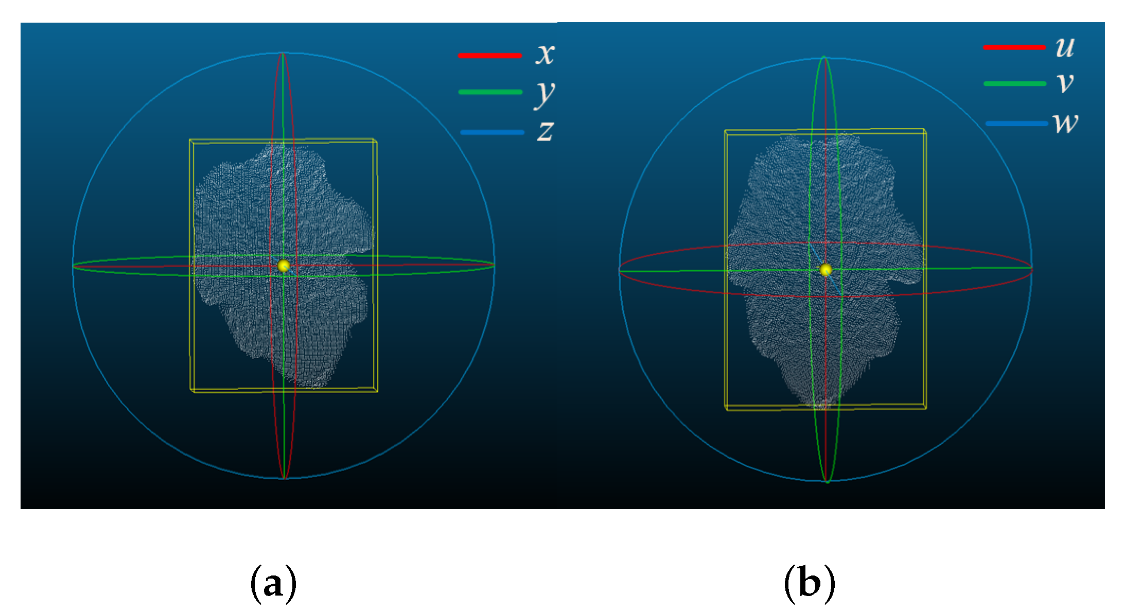
Assuming that the distance of leaf length is greater than leaf width, PCA was used to determine the main diameter axis of the leaf , u is the axis of leaf length, v is the axis of leaf width, and w is the axis of thickness. The bounding box of the leaf is made based on the coordinate system, and the points tangent to the bounding box in the u and v directions are the key points required.
After obtaining the coordinate system, the intersection points of bounding box and leaf point cloud are extracted, which represent the maximum value of leaf extension and as the key points of measuring length and width. Figure 2a represents the coordinate system of the original point cloud, where the red straight line is the x axis, green line is the y axis, and blue line is the z axis; Figure 2b represents the coordinate system of point cloud processed by PCA, where the red straight line is the u axis, green line is the v axis, and blue line is the w axis. Assuming leaf length is greater than leaf width, u is the main axis, v is the secondary main axis, and w is the tertiary main axis. The yellow border of the 3D leaf model in Figure 2 is obtained by the bounding box method. The points intersected with the bounding box in v axis are measuring points of the leaf width, named , . The point where the u axis of the bounding box intersects the bottom of the leaf is , while the point on the other side of leaf length cannot be directly used as the point of the leaf tip. Since eggplant petiole is located in the concave surface of the point cloud, the point where the bounding box intersects with the u axis is not the petiole, so the point needs to be selected manually.
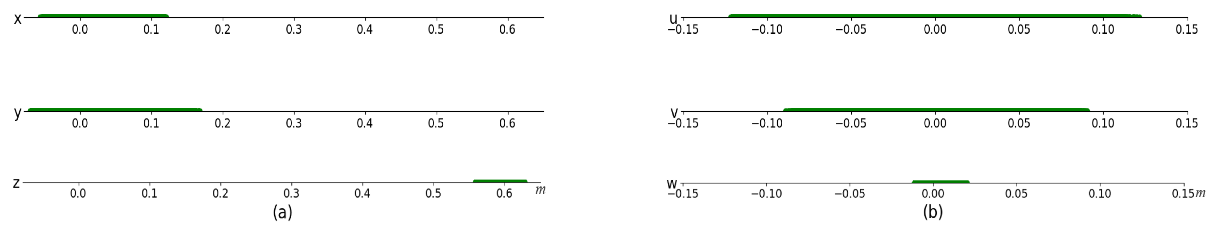
In Figure 3a, the original point cloud is projected onto the coordinate system, and Figure 3b the reconstructed point cloud is projected onto the coordinate system. The PCA algorithm is used to process the point cloud, and the elements are mapped to the main coordinate axis, secondary main coordinate axis, and tertiary main coordinate axis. The coordinate axis of the reconstructed point cloud has regularity, which is related to the decreasing projection density of the leaf length, width, and thickness. Therefore, the reconstructed main coordinate axis u represents the length of the leaf, the secondary main coordinate axis v represents the width, and the tertiary main coordinate axis w represents the thickness.
Algorithm 1 used the PCA algorithm to reconstruct the coordinate system for obtaining the range of interest (RoI) of leaf and the key points of length and width.
| Algorithm 1 The algorithm of obtaining the measurement points of length and width. |
| Require: for i = 1:n do Calculate by Equation (1) end for Calculate covariance matrix by Equation (2) Calculate eigenvalues and eigenvectors of , and express eigenvectors as the coordinate system , Calculate the minimum bounding box for the leaf model in the coordinate system , Define the reconstructed point cloud as , Define the intersection point of the leaf model and the bounding box in v direction as , , Define the intersection point of the leaf model and the bounding box in u direction as , Define the intersection point of the leaf model in u direction as manually. Ensure: |
2.2. Measurement the Length and Width of Leaf
The commonly used three-dimensional length measurement methods are the cross-section and geodesic distance methods. The cross-section method uses the key points and direction vector to find the tangent plane. In this paper, the key points have been obtained according to the bounding box technique, the length plane and width plane are perpendicular to the plane. The longitudinal section intersects the leaf length with a line of intersection, and the value of this line is used as the measured value of leaf length. The cross section intersects the leaf width with a line of intersection, the value of this line is used as the measured value of leaf width. The obtained length and width tangent are curves, which is consistent with the actual measurement method to obtain the curve distance from the starting point to the end point on the leaf according to the given points.
The geodesic distance method is a heuristic method, in which the starting point and the end point of the measurement must be provided to find the line connecting two points according to the shortest path principle, such as A* [49], Dijkstra [50] geodetic distance method. The Dijkstra algorithm is a typical shortest path algorithm, which is used to calculate the shortest path from the starting node to the final node. The Dijkstra algorithm can obtain the optimal solution of the shortest path. For the current point on the path, A* algorithm records the cost to the source point, and the expected cost from the current point to the target point, so it is a depth-first algorithm. The commonly used heuristic functions of A* algorithm include Manhattan, Euclidean and Chebyshev distances [51]. The research object of this paper is a 3D point cloud, which can move along any direction when looking for the next target points, so the Euclidean distance is chosen as the heuristic function of A* algorithm in this paper. The space distance between points is the basis of the shortest distance. The start and end key points of the geodesic distance method are the same as those of the cross-section method, and the length and width of the leaf are calculated by the start and end key points, so there are fluctuations between adjacent point and point when searching for the shortest path.
In this paper, based on the cross-section method, the direction of the section is not perpendicular to the coordinate system, but the plane is constructed according to the point on the leaf closest to the center of the starting point and the end point. This paper proposes to use the cutting-plane method to obtain the intersection line of the leaf as the basis for measuring the length and width. For the leaf length, the starting point and end point were obtained, but to determine a plane, three points which are not on the same straight line are required, so the third point is needed to construct the three-dimensional plane. Similarly, for the leaf width, the starting point and the end point have been obtained by bounding box technology, and the third point is also needed to construct the width plane. The method proposed in this paper is not to calculate the length and width of the leaf according to the point cloud perpendicular to the coordinate system , and the process of coordinate system transformation can be omitted. It needs to specify the starting point and end point to calculate the target points for the leaf point cloud, then determine the tangent plane of length and width.
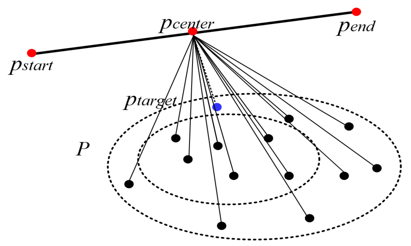
In order to obtain the third point, the midpoint of the line between the starting point and the end point is set as in Equation (3). The point closest to on the leaf point cloud is selected as the third point on the cutting plane in Equation (4). The target point selected in this way can ensure the closest distance to the point , and the three points , and constituted the plane from the three-dimensional leaf model.
where, denotes the coordinates of the point with the smallest distance between and , and d denotes the Euclidean distance of two points. Similarly, when calculating the width tangent plane, the midpoint of the line between the starting point and the end point is in Equation (5). The point closest to is selected as on the leaf model in Equation (6).
In Figure 4, the red points, respectively, represent , , and , while black points represent the 3D leaf model. The point with the smallest distance to is selected as , which is represented in blue.
For the section of leaf length, the three points of , and are on the same straight line, then and and are not on the same straight line, so according to the plane equation, it can be guaranteed that the three points determine a plane. For the section of width, and and are not in a straight line, so here it can be guaranteed that three points define a plane. This process is to compare the distance between the point set and , and select the point p corresponding to the smallest distance as the point . The purpose is to determine a plane through a line and point, and cut a curve through the plane and leaf point cloud surface.
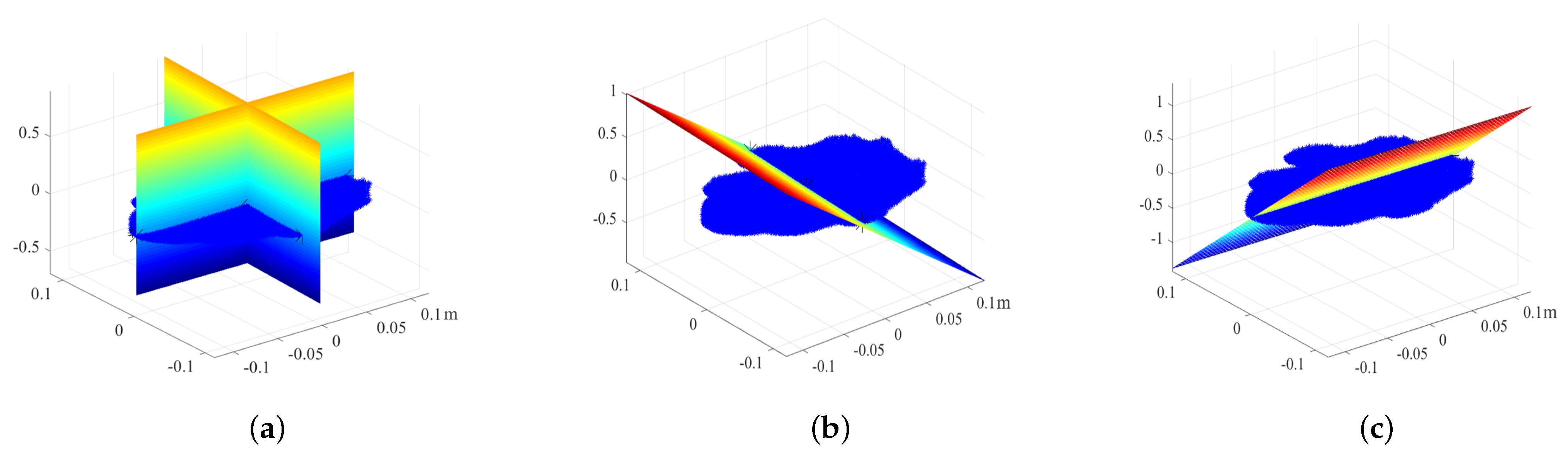
The length and width section of the leaf obtained by the traditional cross-section method is shown in Figure 5a, the coordinate system was reconstructed according to the PCA method, and the length and width planes are perpendicular to the coordinate plane . For the width section, suppose the equation is . The plane through three points that are not on the same line in the equation are , , and . The transverse plane tangent of the leaf is shown in Figure 5b. Suppose the length plane equation is . The plane through three points that are not on the same line in the equation are , , and . The plane tangent of the leaf length in Figure 5c. The section intersects the leaf length with a line, as . Similarly, the section intersects the leaf width with a line, as .
The length and width cut planes obtained by this paper are not perpendicular to the coordinate plane. The essence of our method is to use the tangent plane to cut the model and obtain the point on the intersection line as the basis for calculating the length and width. The leaf model intersects with the length and width planes, which are used to measure the distance of length and width in Algorithm 2.
| Algorithm 2 The algorithm of calculating leaf length and width. |
| Process of calculating leaf length Require: Calculate the midpoint of line using Equation (3). for i = 1:n do Calculate the distance between and as , Find , and the keypoint using Equation (4). end for Calculate the cutting plane of as , Define the tangent point set of leaf model and cutting plane as the length. Ensure: tangent point set Process of calculating leaf width Require: Calculate the midpoint of line using Equation (5). for i = 1:n do Calculate the distance between and as , Find , and the keypoint using Equation (6). end for Calculate the cutting plane of as , Define the tangent point set of leaf model and cutting plane as the width. Ensure: tangent point set |
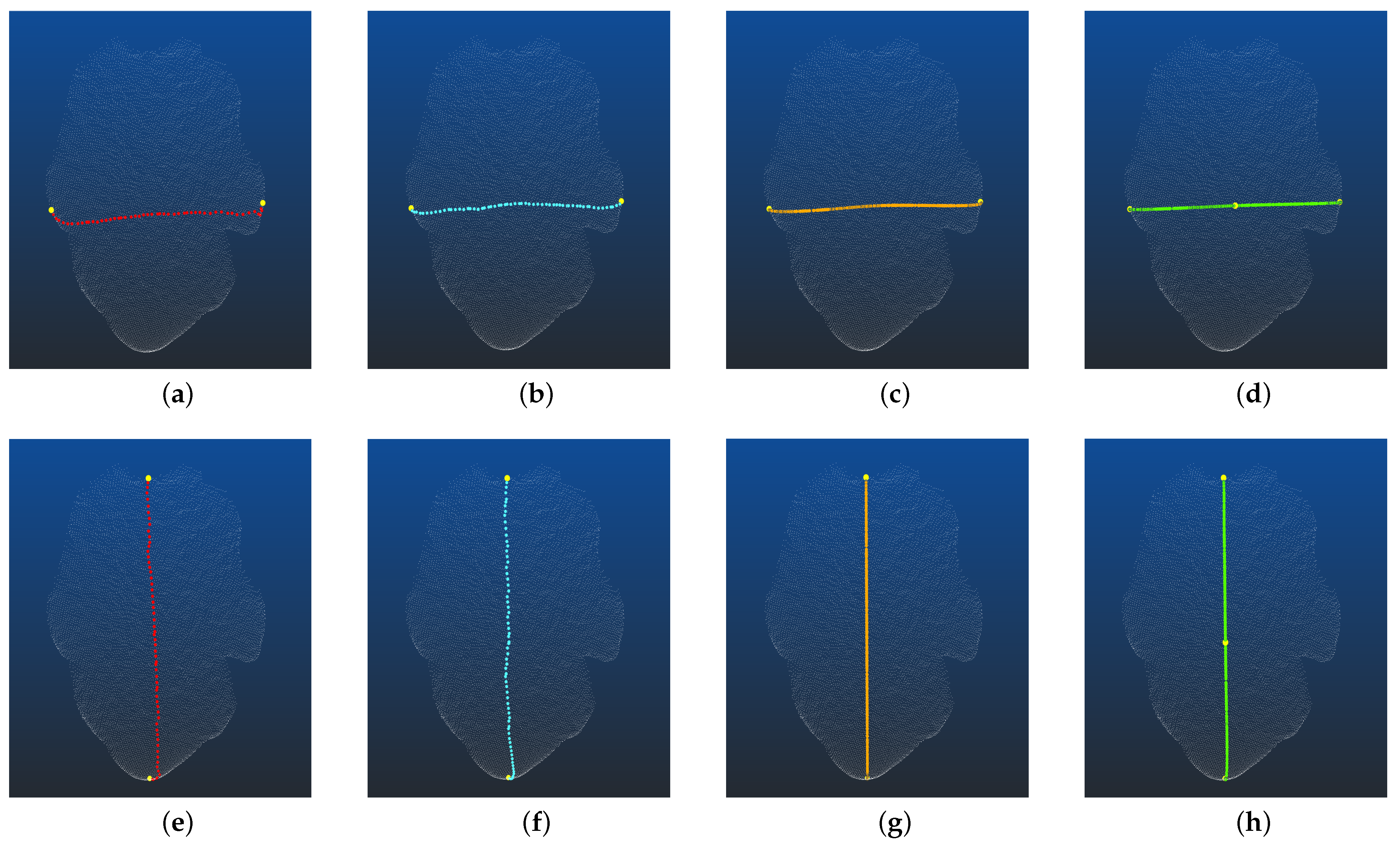
Figure 6 shows the length and width points of eggplant leaves obtained by geodesic distance and cross-section methods. A* and Dijkstra methods were used for geodesic distance method. The starting point and ending point of geodesic distance method and cross-section method are the same, that is , , , . The red line represents the width in Figure 6a and length Figure 6e of the leaf obtained by A* method, the blue line represents the width in Figure 6b and length Figure 6f of the leaf obtained by the Dijkstra method, and the orange line represents the width in Figure 6c and length Figure 6g of the leaf obtained by the cross-section method. The green line represents the width in Figure 6d and length Figure 6h of the leaf obtained by our method. When the starting point and end point are given, our method obtains the key points through the starting and end point.
The geodetic distance method, cross-section method, and the method of this paper have the same starting and end points. The points obtained by A*, Dijkstra method are all on the original point cloud, and the shortest distance from the starting point to the end point obtaining according to the distance between each point of the leaf model. Therefore, the geodetic distance method requires more time, and the time complexity of the Dijkstra method is [52]. The essence of the cross-section method and this paper is to take the intersection point of the section and the model as the key points. The principle of the cross-section method to obtain the plane is based on the starting point, the end point and the vector perpendicular to the coordinate plane. The principle of this paper is based on the starting point, end point and target points. Therefore, in Figure 6d,h, there is starting point, end point and target point indicated by yellow dots.
3. Results
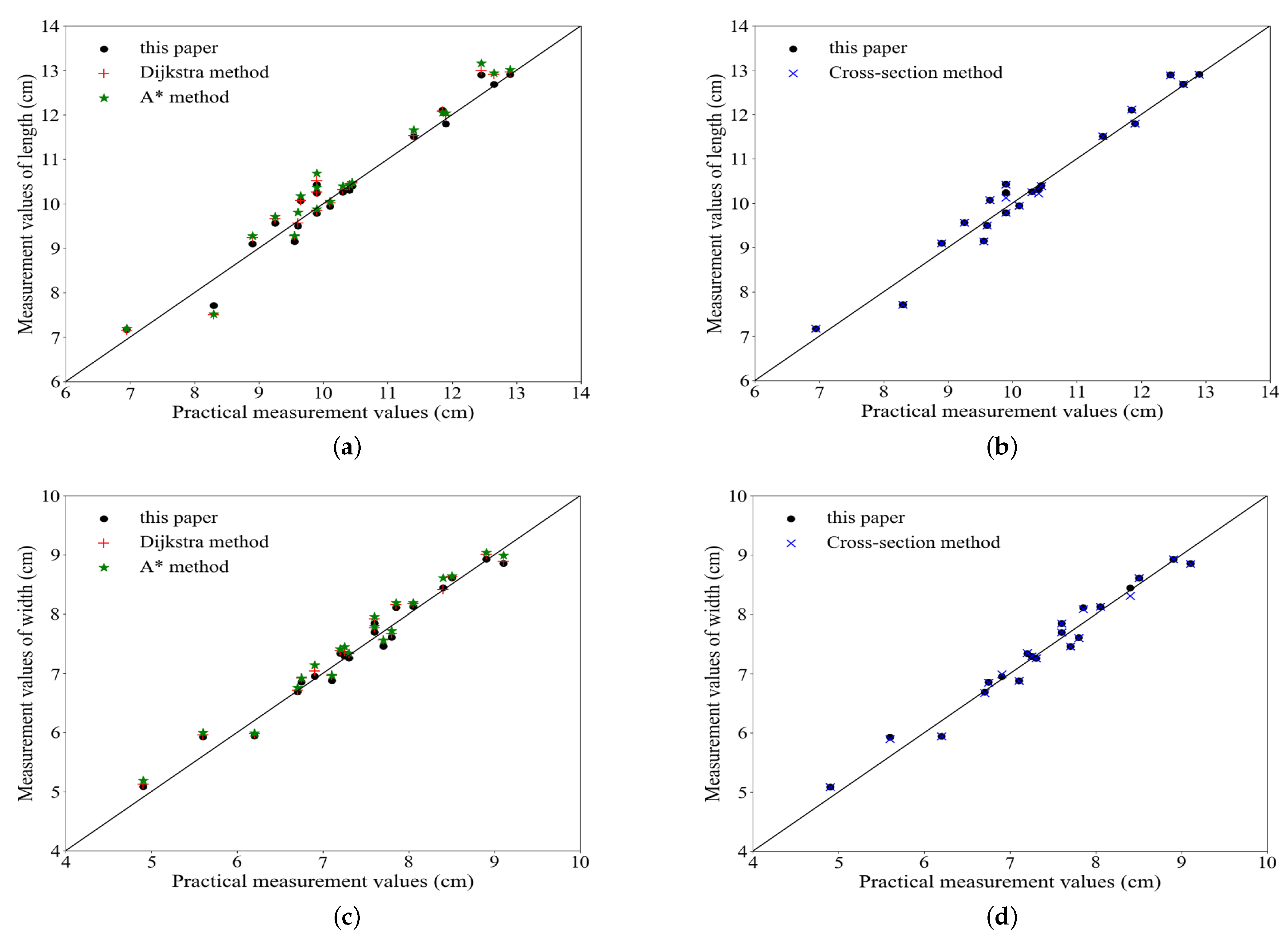
In this paper, 20 three-dimensional eggplant leaves were taken as experimental objects, and obtain the key points of each model , , and . After obtaining the key points and , the length and width were calculated by A*, Dijkstra, cross-section and methods proposed in this paper. For the key point set of cutting plane , it needs to be connected and measured between two adjacent points and by spatial distance. Figure 7 shows the measurement values of length(or width) comparison between our method with A* algorithm, Dijkstra algorithm and cross-section method under certain practical measurement values. The points of the coordinate axis represent the estimated values obtained by the algorithms, while the horizontal coordinate axis represents the actual width and length values. From Figure 7a–d, the method proposed in this paper was compared with A*, Dijkstra and cross-section methods, and the differences with actual values.
The coefficients of determination () of 20 groups of data were calculated to compare the accuracy of each method, where the length calculated by bthe A* method compared with the actual length was 0.930; the value of length calculated by the Dijkstra method compared with the actual length was 0.949; the value of length calculated by the cross-section method compared with the actual length was 0.963; the value of length calculated by this paper compared with the actual length was 0.962; the value of width calculated by the A* method compared with the actual width was 0.956; the value of width calculated by the Dijkstra method and compared with actual width was 0.966; the value of width calculated by the cross-section method compared with the actual width was 0.970; the value of width calculated by this paper compared with the actual width was 0.970; Compared with the errors of the geodetic distance method and cross-section method, this paper’s method with actual values tested in this paper were all within the acceptable range of the study, so these methods can be used to measure the length and width of the leaf. But in terms of time complexity, the geodesic distance needs extra time to compare the distance between points, so the cross-section method and the algorithm in this paper have low time complexity. The algorithm in this paper needs one traversal to find the target point, and the time complexity is . In terms of algorithm complexity, the cross-section method needs to reconstruct the coordinate system to obtain the vector. The algorithm in this paper constructs a spatial plane based on three points that are not on the same straight line, which does not require the process of reconstructing the coordinate system. The accuracy of this paper and cross-section method are higher than geodetic distance method, because all points of the geodetic distance method must be in the model when selecting the shortest path. Our method is similar to the cross-section method, which are both cutting the model by plane, and the key points are obtained through the tangent line.
Compared with a two-dimensional image, a three-dimensional point cloud contains spatial information of the object. This article proves that the geodetic distance and cross-section methods are also suitable for the measurement of the three-dimensional leaf model.
4. Discussion and Conclusions
The geodetic distance method is the process of finding the key points at the shortest distance from the starting point to end point on the original point cloud. It uses the distance relationship between points on the point cloud as the basis for obtaining the shortest distance in the next step. The time complexity of the Dijkstra method is [52], which is related to the density of points. In order to improve the efficiency of the algorithm, the cross-section method is further used to calculate the length and width of the leaf, which directly uses the tangent plane to cut the point cloud to obtain the intersection point. However, this method stipulates that the cutting plane must be perpendicular to the coordinate plane to obtain the dimensional information, so the coordinate system of the point cloud must be processed in advance. Furthermore, it is considered whether the points on the leaf can be directly used to construct the plane, so the starting point, end point and the target point obtained according to formulas (4) and (6) were considered to construct the plane equation. This plane need not be perpendicular to the coordinate plane. It uses the point cloud’s information and the simplicity of the cross-section method.
This paper compares the commonly used three-dimensional measurement methods, such as the geodesic distance and cross section methods, and further proposes our algorithm. The experiment showed that the geodesic distance method (A*, Dijkstra), cross-section method and our method can be used to calculate the actual length and width of the leaf. This algorithm is improved compared to the cross-section method, as it overcomes the problem that the cross-section method must reconstruct the coordinate system. Our measurement method is based on three key points to obtain the section directly, so compared with geodesic distance, it did not need a long time and high space complexity to find the shortest path.
Kinect2.0 was used to collect the point cloud of the leaf, the experimental part of the article did not involve point cloud registration. Therefore, we did not choose leafy vegetables as the object, because the leaves of leafy vegetables are mutually occluded, and cannot obtain the complete leaf point cloud information. Furthermore, we did not extract the rolled leaves as the object, because the rolled leaves cannot obtain complete information through a single depth image. The focus of the research is to compare the geodesic distance, cross-section and improved methods, for the measurement of an individual leaf on the plant, so there is no reconstruction of the plant point cloud, such as structure-from-motion technology and multi-view stereo technology.
Length measurement did not include the length of the petiole, it’s necessary to remove petiole to ensure the accuracy of measurements, so the petiole was removed manually.
For the key points , if the leaf shapes of the research object are needle-shaped or tapered, the petiole is in the bulge of the leaf point cloud, and the bounding box technique can be used to directly obtain the intersection point as the for length measurement, which removes the problem of manually selecting key point . However, due to the particularity of the eggplant leaf’s shape, must still be selected manually.
Leaf parameters have a profound impact on activities such as plant growth and development, so the results reported in this paper on measurement length and width of a 3D leaf point cloud have practical significance.
Author Contributions
Conceptualization, Y.C.; methodology, Y.W.; software, Y.W. and W.G.; validation, X.Z., Y.W. and W.G.; formal analysis, Y.C.; investigation, Y.W. and X.Z.; resources, Y.W. and W.G.; data curation, Y.W.; writing—original draft preparation, Y.W.; writing—review and editing, Y.C.; visualization, Y.W. and X.Z.; supervision, Y.C.; project administration, Y.C.; funding acquisition, Y.C. All authors have read and agreed to the published version of the manuscript.
Funding
This research was funded by the “Research and Development of Greenhouse Cluster Control System”, grant number “s20163081109”.
Acknowledgments
The authors thank the editor and anonymous reviewers for providing helpful suggestions for improving the quality of this manuscript.
Conflicts of Interest
The authors declare no conflict of interest.
Abbreviations
The following abbreviations are used in this manuscript:
| 3D | three-dimensional |
| RoI | Range of Interest |
| PCA | Principal Component Analysis |
References
- Zhou, L. Studies on Image-Based Plant Leaf Parameter Measurement; Hunan University: Changsha, China, 2015. [Google Scholar]
- Thakur, S.; Bawiskar, S.; Singh, S.K.; Shanmugasundaram, M. Autonomous Farming–Visualization of Image Processing in Agriculture. In Inventive Communication and Computational Technologies; Springer: Singapore, 2020. [Google Scholar]
- Lu, S.; Guo, X.; Li, C. Research on Techniques for Accurate Modeling and Rendering 3D Plant Leaf. J. Image Graph. 2009, 14, 731–737. [Google Scholar]
- Hui, F.; Zhu, J.; Hu, P.; Meng, L.; Zhu, B.; Guo, Y.; Li, B.; Ma, Y. Image-based dynamic quantification and high-accuracy 3D evaluation of canopy structure of plant populations. Ann. Bot. 2018, 121, 1079–1088. [Google Scholar] [CrossRef] [PubMed]
- Wu, L.; Long, Y.; Sun, H.; Liu, N.; Wang, W.; Dong, Q. Length Measurement of Potato Leaf using Depth Camera. IFAC Pap. 2018, 51, 314–320. [Google Scholar]
- Li, Y.; Zhang, H.; Yang, Y. A method for obtaing ing plan morphological phenotypic parameters using image processing technology. J. For. Eng. 2020, 5, 128–136. [Google Scholar]
- Xiao, S.; Chai, H.; Shao, K.; Shen, M.; Wang, Q.; Wang, R.; Sui, Y.; Ma, Y. Image-Based Dynamic Quantification of Aboveground Structure of Sugar Beet in Field. Remote Sens. 2020, 12, 269. [Google Scholar] [CrossRef] [Green Version]
- Elnashef, B.; Filin, S.; Lati, R.N. Tensor-based classification and segmentation of three-dimensional point clouds for organ-level plant phenotyping and growth analysis. Comput. Electron. Agric. 2019, 156, 51–61. [Google Scholar] [CrossRef]
- Wu, S.; Wen, W.; Xiao, B.; Guo, X.; Du, J.; Wang, C.; Wang, Y. An Accurate Skeleton Extraction Approach from 3D Point Clouds of Maize Plants. Front. Plant Sci. 2019, 10, 248. [Google Scholar]
- Xiang, L.; Bao, Y.; Lie, T.; Ortiz, D.; Salas-Fernandez, M.G. Automated morphological traits extraction for sorghum plants via 3D point cloud data analysis. Comput. Electron. Agric. 2019, 162, 951–961. [Google Scholar]
- Liang, M. Design and Implementation of Image Software Based on Mobile Terminal for Parameters Measurement of Plant Leaf; Hunan University: Changsha, China, 2018. [Google Scholar]
- Chen, A.; Li, D.; Dong, G. A system for plant leaf parameter measure based on MATLAB. J. China Univ. Metrol. 2010, 21, 310–313. [Google Scholar]
- Rouphael, Y.; Mouneimne, A.H.; Ismail, A.; Gyves, M.D.; Rivera, C.M.; Colla, G. Modeling individual leaf area of rose (Rosa hybrida L.) based on leaf length and width measurement. Photosynthetica 2010, 48, 9–15. [Google Scholar] [CrossRef]
- Shi, P.; Liu, M.; Yu, X.; Gielis, J.; Ratkowsky, D.A. Proportional Relationship between Leaf Area and the Product of Leaf Length and Width of Four Types of Special Leaf Shapes. Forests 2019, 10, 178. [Google Scholar] [CrossRef] [Green Version]
- Zhang, J.; Xie, T.; Yang, C.; Song, H.; Jiang, Z.; Zhou, G.; Zhang, D.; Feng, H.; Xie, J. Segmenting Purple Rapeseed Leaves in the Field from UAV RGB Imagery Using Deep Learning as an Auxiliary Means for Nitrogen Stress Detection. Remote Sens. 2020, 12, 1403. [Google Scholar] [CrossRef]
- Lu, Y.; Xiao, Z.; Yang, H.; Zhou, Q.; Sun, Y. Rice leaf characteristic parameters measurement system based on Android. J. South Agric. 2019, 50, 669–676. [Google Scholar]
- Li, Y.; Li, Y. Fast Algorithm for Extracting Minimum Enclosing Rectangle of Plant Leaves. J. Jiangnan Univ. Sci. Ed. 2015, 14, 273–277. [Google Scholar]
- Wang, J.; Li, C.; Wang, Q.; Wang, B.; Li, F. The Extraction of Leaves’ Aspect Ratio and Boundary Curvature. J. South China Norm. Univ. Natural Ence Ed. 2013, 1, 42–45. [Google Scholar]
- Yuan, W.; Hu, D. Measurement of leaf blade length and width based on moment. Comput. Eng. Appl. 2013, 49, 188–191. [Google Scholar]
- Xiang, Y.; He, Y.; Wei, Y.; Liang, H.; Guo, B. Algorithm for Minimum Bounding Rectangle of Fast Extracting Leaves. Comput. Mod. 2016, 2, 58–61. [Google Scholar]
- Guo, S.; Zhou, L.; Wen, H. Image-based length measurement method of axially symmetric plant leaves with elongated petiole. J. Electron. Meas. Instrum. 2015, 29, 866–873. [Google Scholar]
- Wang, H.; Zhu, D.; Guo, H.; Ma, Q.; Su, W.; Su, Y. Automated calculation of heart girth measurement in pigs using body surface point clouds. Comput. Electron. Agric. 2019, 156, 565–573. [Google Scholar]
- Guo, H.; Ma, X.; Ma, Q.; Wang, K.; Su, W.; Zhu, D. LSSA-CAU: An interactive 3d point clouds analysis software for body measurement of livestock with similar forms of cows or pigs. Comput. Electron. Agric. 2017, 138, 60–68. [Google Scholar]
- Zhou, Y.; Xue, H.; Wang, C.; Jiang, X.; Gao, X.; Bai, J. Reconstruction and Body Size Detection of 3D Sheep Body Model Based on Point Cloud Data. In Proceedings of the International Conference on Computer and Computing Technologies in Agriculture, Jilin, China, 12–15 August 2017; pp. 251–262. [Google Scholar]
- Zhang, X.; Liu, G.; Jing, L.; Si, Y.; Ren, X.; Ma, L. Automatic Extraction Method of Cow’s Back Body Measuring Point Based on Simplification Point Cloud. Trans. Chin. Soc. Agric. Mach. 2019, 50, 267–275. [Google Scholar]
- Li, X.; Chen, M. Algorithm for Extracting End Feature Point of 3D Human Body Model Using Point Cloud Data. In Proceedings of the 2012 International Academic Conference of Art Engineering and Creative Industry(IACAE 2012), Fuzhou, China, 13 October 2012; pp. 20–25. [Google Scholar]
- Liu, T.; Peng, X.; Tan, X. Method of Automatic Measurement of Human Size Based on Depth Camera. J. Chin. Comput. Syst. 2019, 40, 2202–2208. [Google Scholar]
- Tan, X.; Peng, X.; Liu, L.; Xia, Q. Automatic human body feature extraction and personal size measurement. J. Vis. Lang. Comput. 2018, 47, 9–18. [Google Scholar] [CrossRef]
- Zhang, W.; Kong, D.; Wang, S.; Wang, Z. 3D human pose estimation from range images with depth difference and geodesic distance. J. Vis. Commun. Image Represent. 2019, 59, 272–282. [Google Scholar]
- Song, P.; Yang, Z. The Application of 3D Laser Scanning Technology in Earthwork Calculation of High and Steep Slope. Urban Geotech. Investig. Surv. 2019, 2, 63–65. [Google Scholar]
- Yan, H.; Zhu, B.; Wang, J. Application of Unmanned Airborne LIDAR in Mountain Water Conservancy Mapping. Mod. Surv. Mapp. 2019, 42, 48–50. [Google Scholar]
- Maria, V.C.; Jeffrey, B.E. Image-based phenotyping and genetic analysis of potato skin set and color. Crop Sci. 2020, 60, 202–210. [Google Scholar]
- Wang, J.; Zhang, Y.; Gu, R. Research Status and Prospects on Plant Canopy Structure Measurement Using Visual Sensors Based on Three-Dimensional Reconstruction. Agriculture 2020, 10, 462. [Google Scholar] [CrossRef]
- Zhou, L.; Gu, X.; Cheng, S.; Yang, G.; Shu, M.; Sun, Q. Analysis of Plant Height Changes of Lodged Maize Using UAV-LiDAR Data. Agriculture 2020, 10, 146. [Google Scholar] [CrossRef]
- Guo, C.; Zong, Z.; Zhang, X.; Liu, G. Apple tree canopy geometric parameters acquirement based on 3D point clouds. Trans. Chin. Soc. Agric. Eng. 2017, 33, 175–181. [Google Scholar]
- Gongal, A.; Karkee, M.; Amatya, S. Apple fruit size estimation using a 3D machine vision system. Information Processing in Agriculture. Inf. Process. Agric. 2018, 5, 498–503. [Google Scholar]
- Yang, H.; Wang, X.; Sun, G. Three-Dimensional Morphological Measurement Method for a Fruit Tree Canopy Based on Kinect Sensor Self-Calibration. Agronomy 2019, 9, 741. [Google Scholar]
- Zhang, Y.; Teng, P.; Shimizu, Y.; Hosoi, F.; Omasa, K. Estimating 3D Leaf and Stem Shape of Nursery Paprika Plants by a Novel Multi-Camera Photography System. Sensors 2016, 16, 874. [Google Scholar] [CrossRef] [PubMed] [Green Version]
- Feng, Q.; Chen, J.; Li, C.; Fan, P.; Wang, X. Measurement Method of Vegetable Seedling Leaf Morphology Based on Photometric Stereo. Trans. Chin. Soc. Agric. Mach. 2018, 49, 43–50. [Google Scholar]
- Zhang, Y.; Wang, X.; Sun, G.; Li, Y.; Sun, X. Leaves and Stems Measurement of Plants Based on Laser Vision in Greenhouses. Trans. Chin. Soc. Agric. Mach. 2014, 45, 254–259. [Google Scholar]
- Itakura, K.; Hosoi, F. Automatic Leaf Segmentation for Estimating Leaf Area and Leaf Inclination Angle in 3D Plant Images. Sensors 2018, 18, 3576. [Google Scholar] [CrossRef] [Green Version]
- Hu, C.; Pan, Z.; Li, P. A 3D Point Cloud Filtering Method for Leaves Based on Manifold Distance and Normal Estimation. Remote Sens. 2019, 11, 198. [Google Scholar]
- Removing Outliers Using a Conditional or RadiusOutlier Removal. Available online: https://pcl.readthedocs.io/projects/tutorials/en/latest/remove_outliers.html (accessed on 24 June 2020).
- Smoothing and Normal Estimation Based on Polynomial Reconstruction. Available online: https://pcl.readthedocs.io/projects/tutorials/en/latest/resampling.html (accessed on 3 July 2020).
- Principal Component Analysis. Available online: https://www.mathworks.com/help/stats/principal-component-analysis-pca.html (accessed on 12 August 2020).
- Li, W.; Liu, C. Research on Improved PCA-based ICP Point Cloud Registration Algorithm. Ind. Control. Comput. 2020, 33, 11–13. [Google Scholar]
- Zhang, R.; Li, G.; Li, M.; Wang, S. Classification of LiDAR Point Clouds Based on PCA-BP Algorithm. Bull. Surv. Mapp. 2014, 7, 23–26. [Google Scholar]
- Dimitrov, D.; Knauer, C.; Kriegel, K.; Rote, G. Bounds on the quality of the PCA bounding boxes. Comput. Geom. 2009, 42, 772–789. [Google Scholar] [CrossRef] [Green Version]
- Hart, P.E.; Nilsson, N.J.; Raphael, B. A Formal Basis for the Heuristic Determination of Minimum Cost Paths. IEEE Trans. Syst. Sci. Cybern. 1968, 4, 100–107. [Google Scholar] [CrossRef]
- Dijkstra, E.W. A note on two problems in connexion with graphs. Numer. Math. 1959, 1, 269–271. [Google Scholar] [CrossRef] [Green Version]
- Yan, W.; Wu, W. Data Structure (C Language Edition); Tsinghua University Press: Beijing, China, 2011; pp. 186–192. [Google Scholar]
- Du, P.; Tu, C.; Wang, W. Computing Geodesics on Point Clouds. J. Comput. Aided Des. Comput. Graph. 2006, 3, 438–442. [Google Scholar]
Figure 1.
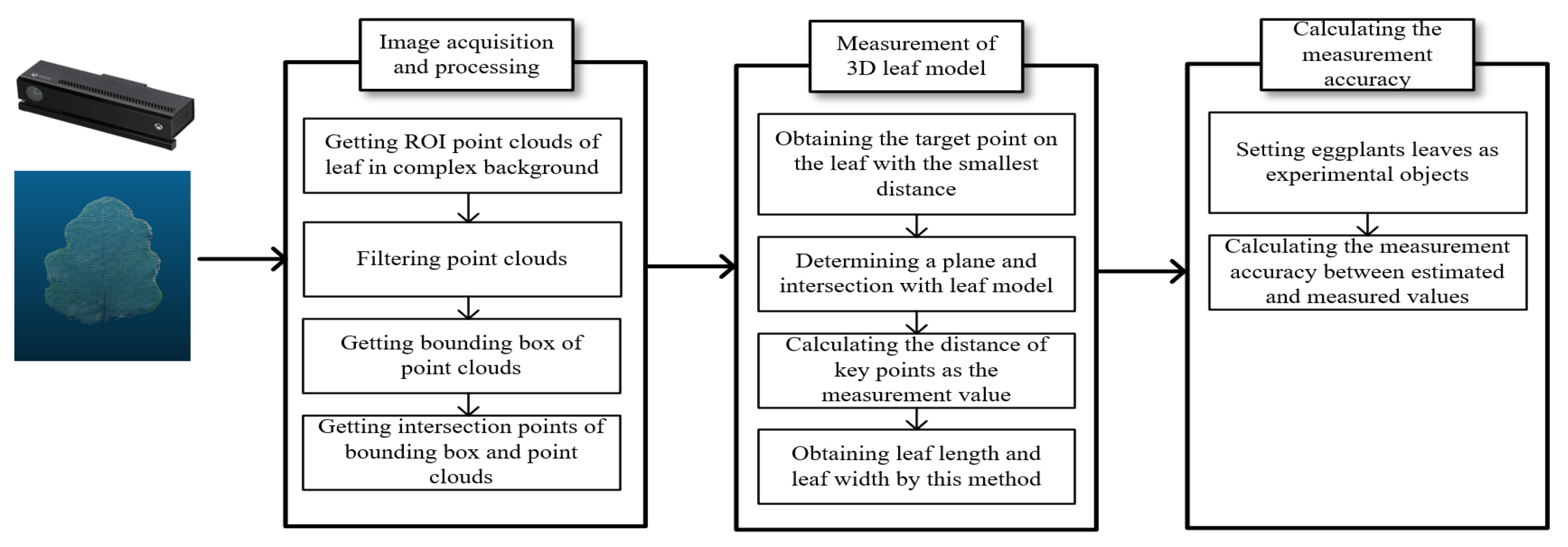
Operation flowchart of the system.

Figure 2.
Coordinate system of leaf point cloud. (a) Original coordinate system of point cloud. (b) Processed coordinate system of point cloud.
Figure 2.
Coordinate system of leaf point cloud. (a) Original coordinate system of point cloud. (b) Processed coordinate system of point cloud.

Figure 3.
Projection of point cloud data onto the coordinate system. (a) Distribution map of the point cloud in the original coordinate system . (b) Distribution map of the point cloud in the reconstructed coordinate system .
Figure 3.
Projection of point cloud data onto the coordinate system. (a) Distribution map of the point cloud in the original coordinate system . (b) Distribution map of the point cloud in the reconstructed coordinate system .

Figure 4.
Determination of the target point by starting and end point.

Figure 5.
Obtaining spatial length and width planes of leaf. (a) Spatial planes of length and width by cross-section method. (b) Spatial plane of width according to this paper. (c) Spatial plane of length according to this paper.
Figure 5.
Obtaining spatial length and width planes of leaf. (a) Spatial planes of length and width by cross-section method. (b) Spatial plane of width according to this paper. (c) Spatial plane of length according to this paper.

Figure 6.
Obtaining the point sets of leaf length and width. (a) Obtaining the key point set of width by A* algorithm. (b) Obtaining the key point set of width by Dijkstra algorithm. (c) Obtaining the key point set of width by cross-section algorithm. (d) Obtaining the key point set of width by our method. (e) Obtaining the key point set of length by A* algorithm. (f) Obtaining the key point set of length by Dijkstra algorithm. (g) Obtaining the key point set of length by cross-section algorithm. (h) Obtaining the key point set of length by our method.

Figure 7.
Comparison of the length and width values measured by algorithms with actual values. (a) Comparison of the geodesic distance method with this paper on leaf length. (b) Comparison of cross-section method with this paper on leaf length. (c) Comparison of geodesic distance method with this paper on leaf width. (d) Comparison of cross-section method with this paper on leaf width.

Publisher’s Note: MDPI stays neutral with regard to jurisdictional claims in published maps and institutional affiliations. |
© 2021 by the authors. Licensee MDPI, Basel, Switzerland. This article is an open access article distributed under the terms and conditions of the Creative Commons Attribution (CC BY) license (http://creativecommons.org/licenses/by/4.0/).
Share and Cite
MDPI and ACS Style
Wang, Y.; Chen, Y.; Zhang, X.; Gong, W. Research on Measurement Method of Leaf Length and Width Based on Point Cloud. Agriculture 2021, 11, 63. https://0-doi-org.brum.beds.ac.uk/10.3390/agriculture11010063
AMA Style
Wang Y, Chen Y, Zhang X, Gong W. Research on Measurement Method of Leaf Length and Width Based on Point Cloud. Agriculture. 2021; 11(1):63. https://0-doi-org.brum.beds.ac.uk/10.3390/agriculture11010063
Chicago/Turabian StyleWang, Yawei, Yifei Chen, Xiangnan Zhang, and Wenwen Gong. 2021. "Research on Measurement Method of Leaf Length and Width Based on Point Cloud" Agriculture 11, no. 1: 63. https://0-doi-org.brum.beds.ac.uk/10.3390/agriculture11010063
Note that from the first issue of 2016, this journal uses article numbers instead of page numbers. See further details here.