Impact of Policy and Factor Intensity on Sustainable Value of European Agriculture: Exploring Trade-Offs of Environmental, Economic and Social Efficiency at the Regional Level


Abstract
:1. Introduction
2. Literature Background
3. Materials and Methods
3.1. Stage 1—Measuring Sustainable Value Based on Regional Average
3.2. Stage 2—Structural Equation Modelling
- We performed tests for the invariance of parameters among the groups, then we fitted 14 separate cross-sectional SEM models for the respective years within the 2004–2017 period, following the procedure applied by Hadrich and Olson [47]. We ran SEM group analyses using the maximum-likelihood method with bootstrapped standard errors (1000 replications) to limit estimation biases resulting, i.a., from heteroscedasticity. The samples in each year within the 2004–2017 period were treated as separate groups of observations. To test the null hypothesis that structural coefficients, structural intercepts and covariances of structural errors were equal across the groups, we performed tests for group invariance of parameters and joint tests for each parameter class. We also tested for the collinearity of the variables in the model and obtained VIF results below 2 in all cases. The above tests suggested that we could not impose constraints on any parameters, which means it was not possible to assume that they were equal across the groups, so we performed 14 separate SEM estimations. It is worth noting that the PGsubs coefficients and both of the covariances for ECONsust (with ENVsust and SOCsust) were the only invariant parameters. Table 4 depicts the SEM results with bootstrapped standard errors (1000 replications). We tested goodness-of-fit and analysed the modification indices. Our SEM models (Table 4) were saturated and full rank (i.e., it had the best possible fit), so the Chi-square measure (the model vs. the saturated model) was close to 0, and the fit indicators from Table 5 (TLI, CFI, RMSEA and SRMR) also achieved the best possible values.
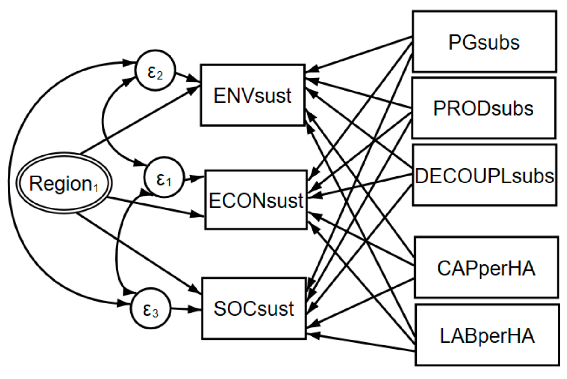
- We estimated multilevel GSEM with a random intercept [49] at the region level using a full panel of 1750 observation (125 regions × 14 years) to capture region-specific random effects. This approach can be described as a kind of variance component model [49], and brings an outcome comparable to a panel regression with random effects (Figure 2); hence, it allows us to interpret the coefficients for a time series.
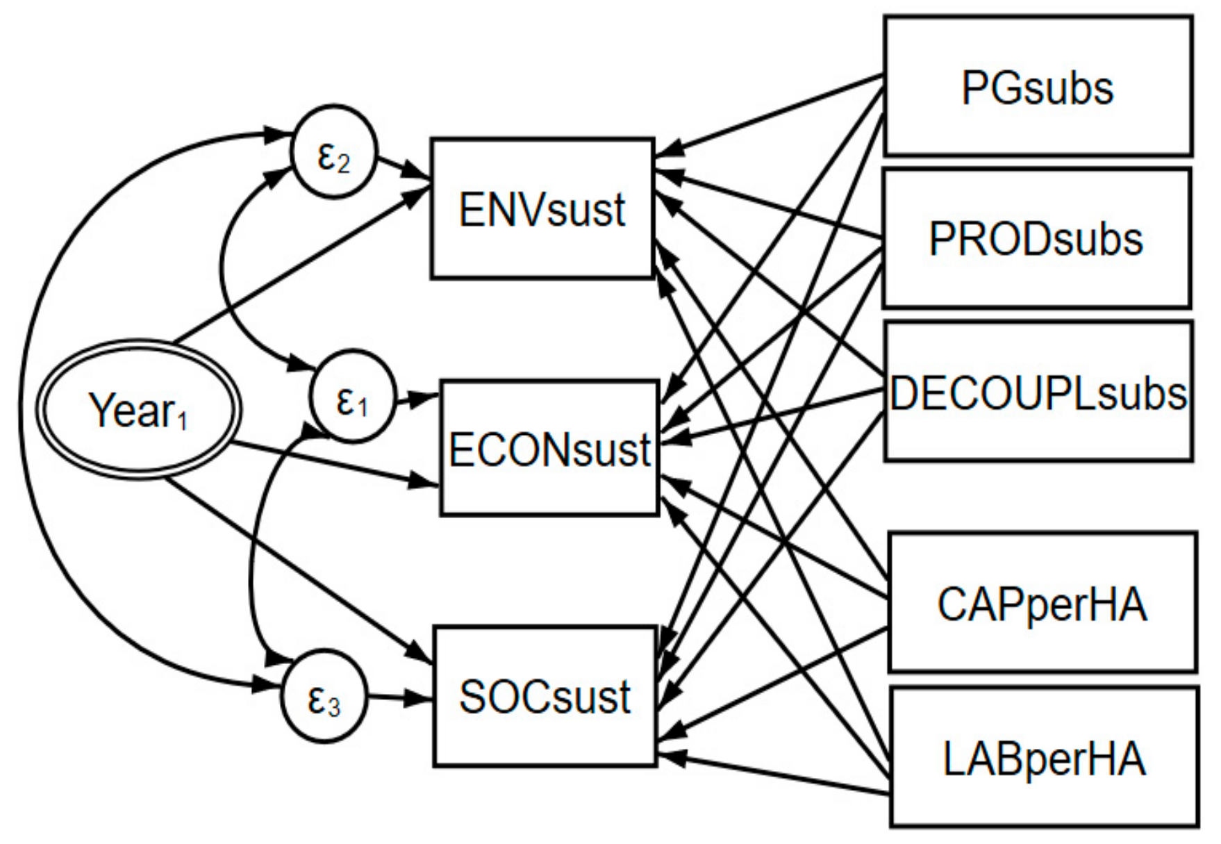
- Finally, we again estimated the GSEM with a random intercept, but this time at the year level, also using the full panel. This is an approach that can be employed for cross-sectional interpretation. We added a random effect measurement (i.e., a multilevel latent variable; see Figure 3) to the model that is constant within a year and varies across years. This is akin to introducing the average level of variables from each year into the model in order to capture the time effect and allow for a cross-sectional interpretation of the panel data.
4. Results
4.1. Descriptive Statistics
4.2. Cross-Sectional SEM Results for Respective Years within 2004–2017
4.3. Multilevel GSEM with Random Region and Year Effect
5. Discussion
6. Conclusions
Author Contributions
Funding
Institutional Review Board Statement
Informed Consent Statement
Data Availability Statement
Conflicts of Interest
References
- Czyżewski, B.; Matuszczak, A.; Muntean, A. Approaching environmental sustainability of agriculture: Environmental burden, eco-efficiency or eco-effectiveness. Agric. Econ. Czech 2019, 65, 299–306. [Google Scholar] [CrossRef]
- Glavič, P.; Lukman, R. Review of sustainability terms and their definitions. J. Clean. Prod. 2007, 15, 1875–1885. [Google Scholar] [CrossRef]
- Shearman, R. The meaning and ethics of sustainability. Environ. Manag. 1990, 14, 1–8. [Google Scholar] [CrossRef]
- Harris, J. Basic Principles of Sustainable Development; Working Paper 00-04. Global Development and Environment Institute, Tufts University, 2000. Available online: https://sites.tufts.edu/gdae/files/2019/10/00-04Harris-BasicPrinciplesSD.pdf (accessed on 22 May 2020).
- Connelly, J.; Smith, G.; Benson, D.; Saunders, C. Politics and the Environment: From Theory to Practice, 2nd ed.; Routledge: New York, NY, USA, 2002. [Google Scholar]
- Waas, T.; Hugé, J.; Verbruggen, A.; Wright, T. Sustainable Development: A Bird’s Eye View. Sustainability 2011, 3, 1637–1661. [Google Scholar] [CrossRef] [Green Version]
- Lauwers, L. Justifying the incorporation of the materials balance principle into frontier-based eco-efficiency models. Ecol. Econ. 2009, 68, 1605–1614. [Google Scholar] [CrossRef]
- Repar, N.; Jan, P.; Dux, D.; Nemecek, T.; Doluschitz, R. Implementing farm-level environmental sustainability in environmental performance indicators: A combined global-local approach. J. Clean. Prod. 2016. [Google Scholar] [CrossRef] [Green Version]
- van Grinsven, H.; van Eerdt, M.; Westhoek, H.; Kruitwagen, S. Benchmarking Eco-Efficiency and Footprints of Dutch Agriculture in European Context and Implications for Policies for Climate and Environment. Front. Sustain. Food Syst. 2019, 3, 3–13. [Google Scholar] [CrossRef] [Green Version]
- Rizov, M.; Pokrivcak, J.; Ciaian, P. CAP Subsidies and Productivity of the EU Farms. J. Agric. Econ. 2013, 64, 537–557. [Google Scholar] [CrossRef]
- Moutinho, V.; Robaina, M.; Macedo, P. Economic-environmental efficiency of European agriculture—A generalized maximum entropy approach. Agric. Econ. Czech 2018, 64, 423–435. [Google Scholar]
- Bartová, L.; Fendel, P.; Matejková, E. Eco-efficiency in agriculture of European Union member states. Roczniki (Annals) 2018, 4. [Google Scholar] [CrossRef]
- Rybaczewska-Błażejowska, M.; Gierulski, W. Eco-Efficiency Evaluation of Agricultural Production in the EU-28. Sustainability 2018, 10, 4544. [Google Scholar]
- Dudu, H.; Kristkova, Z. Impact of CAP Pillar II Payments on Agricultural Productivity. In Proceedings of the XV EAAE Congress “Towards Sustainable Agri-food Systems: Balancing between Markets and Society”, Parma, Italy, 29 August–1 September 2017. [Google Scholar]
- Gotch, A.; Ciaian, P.; Bielza, M.; Terres, J.-M.; Röder, N.; Himics, M.; Salputra, G. EU-Wide Economic and Environmental Impacts of CAP Greening with High Spatial and Farm-Type Detail. J. Agric. Econ. 2017, 68, 651–681. [Google Scholar]
- Figge, F.; Hahn, T. Sustainable Value Added—Measuring Corporate Contributions to Sustainability Beyond Eco-Efficiency. Ecol. Econ. 2004, 48, 173–187. [Google Scholar] [CrossRef]
- Kuosmanen, T.; Kuosmanen, N. How not to measure sustainable value (and how one might). Ecol. Econ. 2009, 69, 235–243. [Google Scholar] [CrossRef]
- Salois, M.J.; Livanis, G.; Moss, C.B. Estimation of Production Functions using Average Data. In Proceedings of the Southern Agricultural Economics Association Annual Meetings, Orlando, FL, USA, 5–8 February 2006. [Google Scholar]
- Felipe, J.; McCombie, J. Problems with Regional Production Functions and Estimates of Agglomeration Economies: A Caveat Emptor for Regional Scientists; Working Paper No. 725; Levy Economics Institute: New York, NY, USA, 2012. [Google Scholar]
- Felipe, J.; McCombie, J. Agglomeration Economies, Regional Growth, and the Aggregate Production Function: A Caveat Emptor for Regional Scientists. Spat. Econ. Anal. 2012, 7, 461–484. [Google Scholar] [CrossRef]
- Staniszewski, J. Attempting to Measure Sustainable Intensification of Agriculture in Countries of the European Union. J. Environ. Prot. Ecol. 2018, 19, 949–957. [Google Scholar]
- Xing, Z.; Wang, J.; Zhang, J. Expansion of environmental impact assessment for eco-efficiency evaluation of China’s economic sectors: An economic input-output based frontier approach. Sci. Total Environ. 2018, 635, 284–293. [Google Scholar] [CrossRef]
- Picazo-Tadeo, A.; Gómez-Limón, J.; Reig-Martínez, E. Assessing farming eco-efficiency: A Data Envelopment Analysis approach. J. Environ. Manag. 2011, 92, 1154–1164. [Google Scholar] [CrossRef]
- Picazo-Tadeo, A.; Beltrán-Esteve, M.; Gómez-Limón, J. Assessing eco-efficiency with directional distance functions. Eur. J. Oper. Res. 2012, 220, 798–809. [Google Scholar] [CrossRef]
- Berre, D.; Vayssières, J.; Boussemart, J.; Leleu, H.; Tillard, E.; Lecomte, P. A methodology to explore the determinants of eco-efficiency by combining an agronomic whole-farm simulation model and efficient frontier. Environ. Model. Softw. 2015, 71, 46–59. [Google Scholar] [CrossRef]
- Gadanakis, Y.; Bennett, R.; Park, J.; Areal, F. Evaluating the sustainable intensification of arable farms. J. Environ. Manag. 2015, 150, 288–298. Available online: http://centaur.reading.ac.uk/37916/1/Final_SI_Yiorgos_Gadanakis.pdf (accessed on 12 December 2020). [CrossRef] [PubMed] [Green Version]
- Pérez Urdiales, M.; Oude Lansink, A.; Wall, A. Eco-efficiency Among Dairy Farmers: The Importance of Socio-economic Characteristics and Farmer Attitudes. Environ. Resour. Econ. 2016, 64, 559–574. [Google Scholar] [CrossRef]
- Bonfiglio, A.; Arzeni, A.; Bodini, A. Assessing eco-efficiency of arable farms in rural areas. Agric. Syst. 2017, 151, 114–125. [Google Scholar] [CrossRef]
- Czyżewski, B.; Matuszczak, A.; Grzelak, A.; Guth, M.; Majchrzak, A. Environmental sustainable value in agriculture revisited: How does Common Agricultural Policy contribute to eco-efficiency? Sustain. Sci. 2020. [Google Scholar] [CrossRef]
- Wrzaszcz, W.; Prandecki, K. Economic Efficiency of Sustainable Agriculture. Probl. Agric. Econ. 2015, 343, 15–36. [Google Scholar]
- Chatzinikolaou, P.; Manos, B.; Bournaris, T. Classification of rural areas in Europe using social sustainability indicators. In Proceedings of the 2012 First Congress, Italian Association of Agricultural and Applied Economics (AIEAA), Trento, Italy, 4–5 June 2012. [Google Scholar]
- Subić, J.; Jeločnik, M.; Jovanović, M. Evaluation of social sustainability of agriculture within the Carpathians in the Republic of Serbia. Manag. Econ. Eng. Agric. Rural Dev. 2013, 13, 411–416. [Google Scholar]
- Basiago, A. Economic, social, and environmental sustainability in development theory and urban planning practice. Environmentalist 1999, 19, 145–161. [Google Scholar] [CrossRef]
- Weingaertner, C.; Moberg, A. Exploring Social Sustainability: Learning from perspectives on Urban Development and Companies and Products. Sustain. Dev. 2014, 22, 122–133. [Google Scholar] [CrossRef] [Green Version]
- Littig, B.; Griessler, E. Social sustainability: A catchword between political pragmatism and social theory. Int. J. Sustain. Dev. 2005, 8, 65–79. [Google Scholar] [CrossRef] [Green Version]
- Figge, F.; Hahn, T. The Cost of Sustainability Capital and the Creation of Sustainable Value by Companies. J. Ind. Ecol. 2005, 9, 47–58. [Google Scholar] [CrossRef]
- Grzelak, A.; Guth, M.; Matuszczak, A.; Czyżewski, B.; Brelik, A. Approaching the environmental sustainable value in agriculture: How factor endowments foster the eco-efficiency. J. Clean. Prod. 2019, 241, 118304. [Google Scholar] [CrossRef]
- Liesen, A.; Müller, F.; Figge, F.; Hahn, T. Sustainable Value Creation by Chemical Companies; Sustainable Value Research Ltd.: Belfast, UK, 2009; Available online: https://www.sustainablevalue.com/downloads/sustainablevaluecreationbychemicalcompanies.pdf (accessed on 13 December 2020).
- Coelli, T.; Rao, D. Total factor productivity growth in agriculture: A Malmquist index analysis of 93 countries, 1980–2000. Agric. Econ. 2005, 32, 115–134. [Google Scholar] [CrossRef] [Green Version]
- Zhu, J. Multiplier and Slack-based Models. Quantitative Models for Performance Evaluation and Benchmarking: International Series in Operations Research & Management Science; Springer: Boston, MA, USA, 2008; Volume 126, pp. 43–62. [Google Scholar]
- Farrell, M. The Measurement of Productive Efficiency. J. R. Stat. Soc. Ser. A 1957, 120, 253–290. [Google Scholar] [CrossRef]
- EUFADN. 2020. Available online: https://ec.europa.eu/agriculture/rica/ (accessed on 15 September 2020).
- Latruffe, L.; Diazabakana, A.; Bockstaller, C.; Desjeux, Y.; Finn, J.; Kelly, E.; Ryan, M.; Uthes, S. Measurement of sustainability in agriculture: A review of indicators. Stud. Agric. Econ. 2016, 118, 123–130. [Google Scholar] [CrossRef]
- Skrondal, A.; Rabe-Hesketh, S. Generalized Latent Variable Modeling: Multi-Level, Longitudinal and Structural Equation Models; Chapman and Hall: Boca Raton, FL, USA, 2004. [Google Scholar]
- Kline, R. Principles and Practice of Structural Equation Modeling; The Guilford Press: New York, NY, USA, 2011. [Google Scholar]
- OECD. Eco-Efficiency; OECD Publishing: Paris, France, 2008. [Google Scholar]
- Hadrich, J.; Olson, F. Joint measure of farm size and farm performance: A confirmatory factor analysis. Agric. Financ. Rev. 2011, 71, 295–309. [Google Scholar] [CrossRef]
- Brown, T.; Moore, M. Confirmatory Factor Analysis. In Handbook of Structural Equation Modeling; Hoyle, R., Ed.; The Guilford Press: New York, NY, USA, 2012; pp. 361–379. [Google Scholar]
- StataCorp. Stata: Release 13. Statistical Software; StataCorp LP: College Station, TX, USA, 2013. [Google Scholar]
- West, S.; Taylor, A.; Wu, W. Model Fit and Model Selection in Structural Equation Modeling. In Handbook of Structural Equation Modeling; Hoyle, R., Ed.; The Guilford Press: New York, NY, USA, 2012; pp. 209–231. [Google Scholar]
- Olley, G.; Pakes, A. The Dynamics of Productivity in the Telecommunications Equipment Industry. Econometrica 1996, 64, 1263–1297. [Google Scholar] [CrossRef]
- Hennessy, D. The Production Effects of Agricultural Income Support Policies under Uncertainty. Am. J. Agric. Econ. 1998, 80, 46–57. [Google Scholar] [CrossRef]
- Ciaian, P.; Swinnen, J. Credit Market Imperfections and the Distribution of Policy Rents. Am. J. Agric. Econ. 2009, 91, 1124–1139. [Google Scholar] [CrossRef] [Green Version]
- Banga, R. Impact of Green Box Subsidies on Agricultural Productivity, Production and International Trade; Background Paper No. RVC-11; Unit of Economic Cooperation and Integration Amongst Developing Countries [ECIDC] UNCTAD: New York, NY, USA, 2018; pp. 15–21. [Google Scholar]
- Manos, B.; Bournaris, T.; Chatzinikolaou, P. Impact assessment of CAP policies on special sustainability in rural areas: An application in Northern Greece. Oper. Res. 2011, 11, 77–92. [Google Scholar]
- Czyżewski, B.; Czyżewski, A.; Kryszak, L. The Market Treadmill against Sustainable Income of European Farmers: How the CAP Has Struggled with Cochrane’s Curse. Sustainability 2019, 11, 791. [Google Scholar]
- Cantore, N.; Kennan, J.; Page, S. CAP Reform and Development: Introduction, Reform Options and Suggestions for Further Research; Overseas Development Institute: London, UK, 2011. [Google Scholar]
- Brady, M.; Hristov, J.; Höjgård, S.; Jansson, T.; Johansson, H.; Larsson, C.; Nordin, I.; Rabinowicz, E. Impacts of Direct Payments—Lessons for CAP Post-2020 from A Quantitative Analysis; Report No. 2017:2; AgriFood Economics Centre: Lund, Sweden, 2017. [Google Scholar]
- European Commission. CAP Specific Objectives…Explained; DG Agri: Brussels, Belgium, 2018. [Google Scholar]
- Wigier, M.; Kowalski, A. The Common Agricultural Policy of the European Union—The Present and the Future; EU Member States Point of View; Institute of Agricultural and Food Economics—National Research Institute: Warsaw, Poland, 2018. [Google Scholar]
- Guth, M.; Smędzik-Ambroży, K.; Czyżewski, B.; Stępień, S. The Economic Sustainability of Farms under Common Agricultural Policy in the European Union Countries. Agriculture 2020, 10, 34. [Google Scholar] [CrossRef] [Green Version]
- Baer-Nawrocka, A. Impact of the Common Agricultural Policy on Income Effects in Agriculture of New Member Countries (Wpływ Wspólnej Polityki Rolnej na Efekty Dochodowe w Rolnictwie Nowych Krajów Członkowskich); Warsaw University of Life Sciences—SGGW Faculty of Economic Sciences: Warsaw, Poland, 2013; Volume 9. [Google Scholar]
- Poczta-Wajda, A. Agricultural Support Policy and the Problem of Income Deprivation of Farmers in Countries with Different Levels of Development [Polityka Wspierania Rolnictwa a Problem Deprywacji Dochodowej Rolników w Krajach o Różnym Poziomie Rozwoju]; PWN: Warsaw, Poland, 2017. [Google Scholar]
- García-Germán, S.; Bardají, I.; Garrido, A. Do increasing prices affect food deprivation in the European Union? Span. J. Agric. Res. 2018, 16, e0103. [Google Scholar] [CrossRef] [Green Version]
- You, J.; Wang, S.; Roope, L. Intertemporal deprivation in rural china: Income and nutrition. J. Econ. Inequal. 2018, 16, 61–101. [Google Scholar] [CrossRef] [Green Version]
- Prus, P. Farmers’ Opinions about the Prospects of Family Farming Development in Poland. In Proceedings of the 2018 International Conference Economic Science for Rural Development, Jelgava, Latvija, 9–11 May 2018; pp. 267–274. [Google Scholar]
- Grovermann, C.; Wossen, T.; Muller, A.; Nichterlein, K. Eco-efficiency and agricultural innovation systems in developing countries: Evidence from macro-level analysis. PLoS ONE 2019, 14, e0214115. [Google Scholar] [CrossRef] [Green Version]
- Porter, M.; van der Linde, C. Green and Competitive: Ending the Stalemate. In The Dynamics of the Eco-Efficient Economy: Environmental Regulation and Competitive Advantage; Harvard Business Review (September–October); Edward Elgar Publishing Limited: Cheltenham, UK, 1995; pp. 120–134. [Google Scholar]
- De Santis, R.; Lasinio, C. Environmental Policies, Innovation and Productivity in EU; LEQS Discussion Paper No. 100; The European Institute: Washington, DC, USA, 2015. [Google Scholar]
- Caiado, R.; de Freitas Dias, R.; Mattos, L.; Quelhas, O.; Leal Filho, W. Towards sustainable development through the perspective of eco-efficiency—A systematic literature review. J. Clean. Prod. 2017, 165, 890–904. [Google Scholar] [CrossRef]
- Nikolov, D.; Manos, B.; Chatzinikolaou, N.; Bournaris, T.; Kiomourtzi, F. Influence of CAP on Social Sustainability in Greek and Bulgarian Areas. In Proceedings of the 132nd Seminar of the EAEE, Skopje, Republic of Macedonia, 25–27 October 2012. [Google Scholar]
- Omann, I.; Spangenberg, J. Assessing Social Sustainability: The Social Dimension of Sustainability in a Socio-Economic Scenario. In Proceedings of the 7th Biennial Conference of the International Society for Ecological Economics, Sousse, Tunisia, 6–9 March 2002. [Google Scholar]
- Dobbs, T.; Pretty, J. Case Study of agri-environmental payments: The United Kingdom. Ecol. Econ. 2008, 65, 765–775. [Google Scholar] [CrossRef]
- Pawłowska-Tyszko, J. CAP and agricultural sustainability financial instruments. In Proceedings of the 142nd EAAE Seminar: Growing Success? Agricultural and Rural Development in an Enlarged EU, Budapest, Hungary, 29–30 May 2014. [Google Scholar]
- Chabé-Ferret, S.; Subervie, J. Econometric methods for estimating the additional effects of agri-environmental schemes on farmers’ practices. In Evaluation of Agri-Environmental Policies: Selected Methodological Issues and Case Studies; OECD: Paris, France, 2012; pp. 185–198. [Google Scholar]
- Van Passel, S.; Nevens, F.; Mathijs, E.; Van Huylenbroeck, G. Measuring farm sustainability and explaining differences in sustainable efficiency. Ecol. Econ. 2007, 62, 149–161. [Google Scholar] [CrossRef]
- Van Passel, S.; Van Huylenbroeck, G.; Lauwers, L.; Mathijs, E. Sustainable Value Assessment of Farms Using Frontier Efficiency Benchmarks. J. Environ. Manag. 2009, 90, 3057–3069. [Google Scholar] [CrossRef] [Green Version]
- Paolotti, L.; Del Campo Gomis, F.J.; Agullo Torres, A.M.; Massei, G.; Boggia, A. Territorial sustainability evaluation for policy management: The case study of Italy and Spain. Environ. Sci. Policy 2019, 92, 207–219. [Google Scholar] [CrossRef]


| No. | Relation | Expected Sign | SEM/GSEM Results | Conclusions |
|---|---|---|---|---|
| H1 | Subsidies for public goods have a negative impact on economic sustainability. | − | Significant negative (−) | H1 accepted |
| H2 | Production subsidies have a positive impact on economic sustainability. | + | Significant negative (−) | H2 rejected |
| H3 | Decoupled payments contribute positively to gaining economic sustainability. | + | Significant negative (−) | H3 rejected |
| H4 | Bigger capital intensity fosters economic sustainability. | + | Significant positive (+) | H4 accepted |
| H5 | Bigger labour intensity negatively affects the economic sustainability. | − | Insignificant negative | H5 inconclusive |
| H6 | Subsidies for public goods contributes positively to environmental sustainability. | + | Significant positive (+) | H6 accepted |
| H7 | Production subsidies have a negative impact on environmental sustainability. | − | Significant negative (−) | H7 accepted |
| H8 | Decoupled payments contribute positively to environmental sustainability. | + | Significant negative (−) | H8 rejected |
| H9 | Bigger capital intensity lowers environmental sustainability. | − | Significant positive (+) | H9 rejected |
| H10 | Bigger labour intensity affects positively environmental sustainability. | + | Significant negative (−) | H10 rejected |
| H11 | Subsidies for public goods contributes positively to social sustainability. | + | Significant negative (−) | H11 rejected |
| H12 | Production subsidies have positive impact on social sustainability. | + | Significant negative (−) | H12 rejected |
| H13 | Decoupled payments contribute positively to social sustainability. | + | Significant (+) in cross-section, (−) for dynamics | H13 accepted in cross-sectional approach; rejected in dynamic aspect |
| H14 | Bigger capital intensity fosters social sustainability. | + | Significant positive (+) | H14 accepted |
| H15 | Bigger labour intensity affects positively the social sustainability. | + | Significant negative (−) | H15 rejected |
| H16 | There is a significant negative two-side relation between economic and environmental sustainability. | − | Significant positive (+) | H16 rejected |
| H17 | There is a significant negative two-side relation between environmental and social sustainability. | − | Significant (+) in cross-section, (−) for dynamics | H17 rejected in cross-sectional approach; accepted in dynamic analysis |
| H18 | There is a positive two-side relation between economic and social sustainability. | + | Significant positive (+) | H18 accepted |
| Var. | Statistics | 2004 | 2005 | 2006 | 2007 | 2008 | 2009 | 2010 | 2011 | 2012 | 2013 | 2014 | 2015 | 2016 | 2017 | ** Av. Growth |
|---|---|---|---|---|---|---|---|---|---|---|---|---|---|---|---|---|
| ENV Sust * | Mean | 0.94 * | 0.93 | 1.01 | 0.94 | 0.88 | 0.87 | 0.88 | 0.88 | 0.87 | 0.88 | 0.95 | 0.97 | 0.94 | 0.93 | 1.00 |
| Std. Dev. | 0.28 | 0.26 | 0.27 | 0.32 | 0.28 | 0.30 | 0.27 | 0.26 | 0.26 | 0.27 | 0.26 | 0.26 | 0.26 | 0.25 | ||
| Min | 0.14 | 0.13 | 0.23 | 0.18 | 0.21 | 0.16 | 0.11 | 0.11 | 0.09 | 0.19 | 0.11 | 0.18 | 0.25 | 0.35 | ||
| Max | 1.66 | 1.53 | 1.66 | 2.57 | 1.59 | 1.81 | 1.56 | 1.46 | 1.51 | 1.52 | 1.56 | 1.65 | 1.61 | 1.58 | ||
| ECON sust | Mean | 0.86 | 0.84 | 0.82 | 0.80 | 0.77 | 0.83 | 0.78 | 0.78 | 0.71 | 0.70 | 0.74 | 0.78 | 0.61 | 0.70 | 0.98 |
| Std. Dev. | 0.30 | 0.31 | 0.29 | 0.25 | 0.26 | 0.29 | 0.26 | 0.25 | 0.24 | 0.24 | 0.23 | 0.26 | 0.25 | 0.26 | ||
| Min | 0.31 | 0.31 | 0.32 | 0.29 | 0.31 | 0.35 | 0.29 | 0.29 | 0.26 | 0.17 | 0.28 | 0.30 | 0.19 | 0.26 | ||
| Max | 1.72 | 1.89 | 1.75 | 1.44 | 1.82 | 1.83 | 1.73 | 1.52 | 1.45 | 1.45 | 1.39 | 1.79 | 1.44 | 1.80 | ||
| SOC sust | Mean | 0.70 | 0.62 | 0.56 | 0.49 | 0.54 | 0.60 | 0.61 | 0.59 | 0.53 | 0.51 | 0.56 | 0.65 | 0.68 | 0.64 | 0.99 |
| Std. Dev. | 0.35 | 0.33 | 0.31 | 0.32 | 0.35 | 0.37 | 0.39 | 0.38 | 0.36 | 0.35 | 0.34 | 0.39 | 0.38 | 0.37 | ||
| Min | 0.14 | 0.11 | 0.09 | 0.02 | 0.04 | 0.07 | 0.08 | 0.08 | 0.06 | 0.06 | 0.08 | 0.09 | 0.09 | 0.08 | ||
| Max | 1.41 | 1.65 | 1.64 | 1.53 | 1.68 | 1.67 | 1.76 | 1.83 | 1.72 | 1.66 | 1.39 | 1.70 | 1.63 | 1.71 | ||
| PG subs | Mean | 0.05 | 0.05 | 0.05 | 0.04 | 0.04 | 0.05 | 0.05 | 0.04 | 0.04 | 0.04 | 0.04 | 0.04 | 0.04 | 0.04 | 0.98 |
| Std. Dev. | 0.06 | 0.07 | 0.06 | 0.06 | 0.06 | 0.07 | 0.06 | 0.06 | 0.05 | 0.05 | 0.05 | 0.06 | 0.05 | 0.05 | ||
| Min | 0.00 | 0.00 | 0.00 | 0.00 | 0.00 | 0.00 | 0.00 | 0.00 | 0.00 | 0.00 | 0.00 | 0.00 | 0.00 | 0.00 | ||
| Max | 0.33 | 0.38 | 0.29 | 0.29 | 0.30 | 0.35 | 0.33 | 0.32 | 0.27 | 0.27 | 0.26 | 0.39 | 0.26 | 0.25 | ||
| PROD subs | Mean | 0.17 | 0.11 | 0.06 | 0.05 | 0.05 | 0.06 | 0.05 | 0.04 | 0.03 | 0.03 | 0.03 | 0.04 | 0.03 | 0.03 | 0.88 |
| Std. Dev. | 0.10 | 0.12 | 0.06 | 0.05 | 0.05 | 0.06 | 0.06 | 0.05 | 0.05 | 0.05 | 0.05 | 0.07 | 0.04 | 0.05 | ||
| Min | 0.01 | 0.00 | 0.00 | 0.00 | 0.00 | 0.00 | 0.00 | 0.00 | 0.00 | 0.00 | −0.01 | 0.00 | 0.00 | 0.00 | ||
| Max | 0.62 | 0.59 | 0.40 | 0.34 | 0.33 | 0.33 | 0.38 | 0.30 | 0.34 | 0.33 | 0.40 | 0.57 | 0.25 | 0.26 | ||
| DECOUPL subs | Mean | 0.07 | 0.10 | 0.13 | 0.11 | 0.12 | 0.13 | 0.12 | 0.12 | 0.11 | 0.12 | 0.12 | 0.08 | 0.07 | 0.07 | 1.00 |
| Std. Dev. | 0.05 | 0.08 | 0.08 | 0.07 | 0.07 | 0.07 | 0.06 | 0.06 | 0.05 | 0.05 | 0.05 | 0.06 | 0.03 | 0.03 | ||
| Min | 0.00 | 0.00 | 0.00 | 0.00 | 0.00 | 0.00 | 0.00 | 0.00 | 0.00 | 0.00 | 0.00 | 0.00 | 0.00 | 0.00 | ||
| Max | 0.25 | 0.35 | 0.36 | 0.32 | 0.33 | 0.36 | 0.30 | 0.26 | 0.27 | 0.28 | 0.27 | 0.68 | 0.16 | 0.15 | ||
| CAP perHa | Mean | 3224.7 | 2969.7 | 3024.93 | 2902.50 | 3397.05 | 3569.88 | 3116.50 | 2632.75 | 2909.01 | 3252.92 | 3255.61 | 3144.99 | 2856.30 | 2844.39 | 0.99 |
| Std. Dev. | 3174.97 | 2607.2 | 2265.17 | 2677.71 | 4102.09 | 3985.24 | 2718.54 | 2435.64 | 2991.27 | 3668.07 | 3734.03 | 3179.98 | 2900.90 | 2992.16 | ||
| Min | 487.20 | 503.12 | 469.19 | 333.03 | 481.38 | 518.84 | 501.26 | 494.18 | 493.37 | 499.96 | 398.72 | 501.86 | 527.22 | 559.84 | ||
| Max | 18,849.6 | 23,701 | 12,674.9 | 14,008.9 | 27,010.4 | 26,207.1 | 20,892.4 | 16,848.5 | 20,058.8 | 28,809.9 | 28,567.7 | 20,248.3 | 20,966.0 | 23,916.7 | ||
| LAB perHa | Mean | 147.26 | 132.74 | 131.02 | 137.64 | 154.15 | 167.80 | 158.64 | 129.53 | 135.48 | 153.53 | 152.95 | 141.52 | 121.95 | 123.24 | 0.99 |
| Std. Dev. | 160.13 | 230.86 | 119.51 | 147.75 | 232.82 | 288.18 | 238.64 | 148.58 | 138.43 | 233.89 | 290.81 | 150.59 | 189.80 | 198.83 | ||
| Min | 14.35 | 25.01 | 18.40 | 14.45 | 22.88 | 22.98 | 14.51 | 12.73 | 22.57 | 20.79 | 19.44 | 12.85 | 14.02 | 14.59 | ||
| Max | 931.83 | 2316.5 | 545.38 | 808.73 | 1877.01 | 2349.57 | 2002.79 | 1021.28 | 669.24 | 1809.84 | 2648.42 | 849.84 | 1927.28 | 2034.19 |
| Environmental Efficiency ENVsust: |
| Stock density per ha (SE120) |
| Mineral fertilisers used (SE295) |
| plant-protection products (SE300) |
| Total use of energy (SE345) |
| UAA minus woodland area * (SE075) |
| Social efficiency SOCsust: |
| Unpaid labour input (SE015) |
| Paid labour input (SE020) |
| Wages paid (SE370) |
| Economic efficiency ECONsust: |
| Total used agricultural area (SE025) |
| Buildings (SE450) |
| Machinery (SE455) |
| Breeding Livestock (SE460) |
| Total current assets (SE465) |
| VARIABLES | 2004 | 2005 | 2006 | 2007 | 2008 | 2009 | 2010 | 2011 | 2012 | 2013 | 2014 | 2015 | 2016 | 2017 |
|---|---|---|---|---|---|---|---|---|---|---|---|---|---|---|
| ENVsust | ||||||||||||||
| PGsubs | 0.519 | −0.077 | −0.315 | 0.755 | 1.468 *** | 0.806 ** | 0.908 ** | 1.176 *** | 1.117 *** | 0.702 * | 0.683 * | 1.049 * | 0.745 | 0.311 |
| [0.544] | [0.307] | [0.395] | [0.595] | [0.4867] | [0.393] | [0.358] | [0.342] | [0.397] | [0.423] | [0.399] | [0.572] | [0.460] | [0.571] | |
| PRODsubs | −1.061 *** | −0.632 *** | −0.876 ** | −1.693 ** | −2.758 *** | −2.527 *** | −2.370 *** | −2.576 *** | −2.622 *** | −2.146 *** | −2.094 *** | −1.485 | −2.340 *** | −1.758 *** |
| [0.397] | [0.215] | [0.415] | [0.596] | [0.527] | [0.399] | [0.428] | [0.485] | [0.421] | [0.473] | [0.377] | [0.923] | [0.579] | [0.664] | |
| DECOUPLsubs | −0.213 | −0.733 ** | −1.418 *** | −1.087 *** | −1.226 *** | −1.464 *** | −1.218 *** | −1.149 *** | −1.650 *** | −1.997 *** | −2.748 *** | −1.015 | −3.683 *** | −3.781 *** |
| [0.491] | [0.294] | [0.387] | [0.422] | [0.362] | [0.324] | [0.380] | [0.414] | [0.379] | [0.393] | [0.391] | [1.406] | [0.577] | [0.688] | |
| CAPperHA’000 | 0.008 | 0.029 ** | 0.016 | −0.009 | 0.003 | 0.015 | 0.016 | 0.022 ** | 0.006 | −0.002 | −0.007 | −0.017 | 0.033 *** | 0.034 *** |
| [0.010] | [0.012] | [0.013] | [0.013] | [0.008] | [0.010] | [0.012] | [0.010] | [0.006] | [0.007] | [0.011] | [0.010] | [0.008] | [0.012] | |
| LABperHA’000 | 0.126 | −0.246 | −0.174 | 0.205 | 0.056 | −0.012 | −0.217 | −0.173 | −0.063 | 0.173 | 0.073 | 0.213 | −0.530 ** | −0.680 ** |
| [0.194] | [0.157] | [0.237] | [0.235] | [0.144] | [0.014] | [0.183] | [0.191] | [0.160] | [0.128] | [0.140] | [0.173] | [0.140] | [0.305] | |
| Constant | 1.065 *** | 1.026 *** | 1.236 *** | 1.094 *** | 1.077 *** | 1.131 *** | 1.085 *** | 1.034 *** | 1.093 *** | 1.129 *** | 1.316 *** | 1.079 *** | 1.227 *** | 1.229 *** |
| [0.066] | [0.068] | [0.085] | [0.066] | [0.054] | [0.056] | [0.070] | [0.072] | [0.066] | [0.067] | [0.059] | [0.126] | [0.056] | [0.080] | |
| ECONsust | ||||||||||||||
| Pgsubs | −1.463 ** | −1.502 *** | −1.494 *** | −0.916 ** | −1.021 ** | −0.888 ** | −1.011 ** | −1.198 ** | −1.375 ** | −1.474 *** | −1.543 *** | −2.063 *** | −0.243 | −0.566 |
| [0.577] | [0.466] | [0.457] | [0.431] | [0.44] | [0.379] | [0.405] | [0.508] | [0.558] | [0.501] | [0.505] | [0.617] | [0.489] | [0.656] | |
| PRODsubs | −0.652 * | −0.359 | −0.840 * | −1.405 *** | −1.280 *** | −1.443 *** | −1.136 ** | −0.980 * | −0.897 * | −0.288 | −0.403 | 1.170 | −1.795 ** | −1.450 * |
| [0.426] | [0.233] | [0.484] | [0.437] | [0.48] | [0.384] | [0.442] | [0.577] | [0.483] | [0.465] | [0.521] | [0.849] | [0.617] | [0.840] | |
| DECOUPLsubs | −0.261 | −1.097 *** | −0.551 * | −0.793 ** | −0.508 | −1.327 *** | −1.156 *** | −1.349 *** | −1.425 *** | −1.445 *** | −1.691 *** | −0.953 | −4.218 *** | −4.808 *** |
| [0.604] | [0.334] | [0.310] | [3.10E−01] | [0.329] | [0.312] | [0.368] | [0.369] | [0.365] | [0.404] | [0.442] | [1.040] | [0.614] | [1.014] | |
| CAPpeHA’000 | 0.004 | 0.024 * | 0.038 *** | 0.017 * | 0.009 | 0.017 * | 0.017 * | 0.021 * | 0.011 | 0.001 | 0.012 | 0.006 | −0.027 *** | −0.030 ** |
| [0.008] | [0.014] | [0.012] | [0.001] | [0.007] | [0.009] | [0.011] | [0.012] | [0.010] | [0.009] | [0.010] | [0.008] | [0.009] | [0.015] | |
| LABperHA’000 | 0.135 | −0.373 ** | −0.411 * | −0.169 | −0.178 | −0.091 | −0.150 | −0.314 * | −0.063 | −0.010 | −0.183 | 0.083 | 0.570 *** | 0.514 |
| [0.161] | [0.175] | [0.227] | [0.173] | [0.132] | [0.131] | [0.114] | [0.178] | [0.187] | [0.144] | [0.144] | [0.182] | [0.149] | [0.313] | |
| Constant | 1.034 *** | 1.053 *** | 0.948 *** | 0962 *** | 0.933 *** | 1.091 *** | 0.989 *** | 1.011 *** | 0.935 *** | 0.944 *** | 0.999 *** | 0.873 *** | 0.998 *** | 1.130 *** |
| [0.068] | [0.066] | [0.071] | [0.0049] | [0.049] | [0.054] | [0.064] | [0.061] | [0.063] | [0.065] | [0.060] | [0.096] | [0.060] | [0.106] | |
| SOCsust | ||||||||||||||
| Pgsubs | −0.482 | −0.953 ** | −0.485 | −0.025 | 0.333 | −0.050 | 0.494 | 0.644 | 0.388 | 0.048 | 0.260 | 0.692 | −0.905 | −1.490 |
| [0.619] | [0.404] | [0.540] | [0.556] | [0.608] | [0.538] | [0.657] | [0.681] | [0.740] | [0.636] | [0.751] | [0.818] | [0.766] | [1.187] | |
| PRODsubs | −0.037 | 0.093 | −1.138 * | −1.570 *** | −1.913 *** | −1.637 *** | −2.327 ** | −2.411 ** | −2.151 ** | −1.859 *** | −1.633 ** | −1.749 ** | −0.072 | 0.235 |
| [0.461] | [0.261] | [0.604] | [0.564] | [0.658] | [0.55] | [0.955] | [1.003] | [0.882] | [0.621] | [0.731] | [0.883] | [0.965] | [1.456] | |
| DECOUPLsubs | 2.045 *** | 1.677 *** | 1.116 *** | 1.696 *** | 1.451 *** | 1.065 ** | 0.507 | 0.411 | −0.215 | −0.713 | −1.153 ** | −0.214 | −1.839 ** | −2.112 * |
| [0.614] | [0.382] | [0.409] | [0.40] | [0.452] | [0.442] | [0.536] | [0.582] | [0.545] | [0.511] | [0.483] | [1.110] | [0.961] | [1.172] | |
| CAPpeHA’000 | −0.004 | 0.016 | −0.003 | −0.010 | −0.001 | 0.0003 | 0.014 | 0.036* | 0.011 | −0.001 | 0.000 | −0.004 | 0.060 *** | 0.051 |
| [0.010] | [0.017] | [0.018] | [0.012] | [0.010] | [0.014] | [0.016] | [0.019] | [0.012] | [0.013] | [0.017] | [0.014] | [0.014] | [0.042] | |
| LABperHA’000 | −0.192 | −0.082 | 0.383 | 0.153 | 0.139 | −0.071 | −0.287 | −0.658 ** | −0.113 | 0.208 | −0.025 | 0.143 | −1.394 *** | −1.261 |
| [0.216] | [0.316] | [0.394] | [0.223] | [0.180] | [0.187] | [0.180] | [0.313] | [0.236] | [0.221] | [0.215] | [0.265] | [0.233] | [0.853] | |
| Constant | 0.626 *** | 0.456 *** | 0.457 *** | 0.387 *** | 0.435 *** | 0.569 *** | 0.639 *** | 0.604 *** | 0.596 *** | 0.628 *** | 0.736 *** | 0.694 *** | 0.838 *** | 0.853 *** |
| [0.079] | [0.077] | [0.080] | [0.063] | [0.067] | [0.076] | [0.095] | [0.093] | [0.090] | [0.084] | [0.085] | [0.111] | [0.094] | [0.185] | |
| cov(ENVsust, ECONsust) | 0.013 * | 0.008 | 0.005 | 0.004 | 0.011 *** | 0.011 *** | 0.009 * | 0.014 *** | 0.013 *** | 0.010* | 0.007 | 0.019 *** | 0.009 * | 0.007 |
| [0.008] | [0.007] | [0.005] | [0.005] | [0.005] | [0.005] | [0.005] | [0.005] | [0.005] | [0.006] | [0.005] | [0.006] | [0.003] | [0.005] | |
| cov(ENVsust, SOCsust) | 0.046 *** | 0.042 *** | 0.033 *** | 0.048 *** | 0.048 *** | 0.052 *** | 0.053 *** | 0.053 *** | 0.050 *** | 0.047 *** | 0.035 *** | 0.041 *** | 0.008 * | 0.018 *** |
| [0.008] | [0.007] | [0.006] | [0.009] | [0.008] | [0.009] | [0.008] | [0.008] | [0.007] | [0.007] | [0.006] | [0.008] | [0.005] | [0.007] | |
| cov(ECONsust, SOCsust) | 0.008 | 0.020 *** | 0.015 ** | 0.018 *** | 0.021 *** | 0.019 *** | 0.023 *** | 0.028 *** | 0.027 *** | 0.026 *** | 0.014 ** | 0.026 *** | 0.012 ** | 0.019 *** |
| [0.008] | [0.007] | [0.007] | [0.006] | [0.007] | [0.008] | [0.007] | [0.006] | [0.006] | [0.006] | [0.005] | [0.007] | [0.005] | [0.007] | |
| CD | 0.512 | 0.599 | 0.643 | 0.594 | 0.543 | 0.607 | 0.51 | 0.496 | 0.506 | 0.46 | 0.535 | 0.385 | 0.785 | 0.804 |
| Observations | 111 | 111 | 111 | 124 | 124 | 125 | 125 | 125 | 125 | 125 | 124 | 125 | 124 | 124 |
| Measure | Name | Description | Cut-off for Good Fit |
|---|---|---|---|
| Chi-Square | Model Chi-Square | Tests the null hypothesis that the estimated model is equal to the saturated model, which perfectly reproduces all of the variances, covariances and means of the observed variables. | p-value > 0.05 |
| NFI (TLI) | (Non) Normed-Fit Index Tucker Lewis Index | An NFI of 0.95 indicates the estimate improves the fit by 95% relative to the null model; NNFI is preferable for smaller samples. Sometimes the NNFI is called the Tucker Lewis index (TLI) | NFI ≥ 0.95 NNFI ≥ 0.95 |
| CFI | Comparative Fit Index | A revised form of NFI that is less sensitive to sample size. | CFI ≥ 0.90 |
| RMSEA | Root Mean Square Error of Approximation | A parsimony-adjusted index. Values less than 0.03 represent excellent fit. | RMSEA < 0.08 |
| SRMR | (Standardised) Root Mean Square Residual | The square-root of the difference between the residuals of the sample covariance matrix and the hypothesised model. SRMR is standardised in nature, so it is easier to interpret than RMR. | SRMR < 0.08 |
| CD | Coefficient of Determination | Interpretation is similar to R-square. | Higher is better |
| AIC | Akaike Information Criterion | Assesses the relative quality of statistical models. | Lower is better |
| BIC | Bayesian Information Criterion | Assesses the relative quality of statistical models. | Lower is better |
| Year Random Intercept (1) | Region Random Intercept (2) | |||||
|---|---|---|---|---|---|---|
| Parameters | Coef. | Std. Err. | P > z | Coef. | Std. Err. | P > z |
| ENVsust | ||||||
| PGsubs | 0.496 | 0.122 | 0.000 | 0.388 | 0.110 | 0.000 |
| PRODsubs | −1.299 | 0.104 | 0.000 | −0.898 | 0.078 | 0.000 |
| DECOUPLsubs | −1.397 | 0.099 | 0.000 | −1.743 | 0.082 | 0.000 |
| CAPperHA’000 | 0.011 | 0.003 | 0.000 | 0.007 | 0.002 | 0.002 |
| LABperHA’000 | −0.107 | 0.040 | 0.007 | −0.028 | 0.033 | 0.388 |
| M1[Year/Region] | 0.580 | 0.095 | 0.000 | 2.530 | 0.269 | 0.000 |
| _cons | 1.097 | 0.019 | 0.000 | 1.111 | 0.018 | 0.000 |
| ECONsust | ||||||
| PGsubs | −1.449 | 0.117 | 0.000 | −1.647 | 0.117 | 0.000 |
| PRODsubs | −0.345 | 0.106 | 0.001 | 0.045 | 0.091 | 0.619 |
| DECOUPLsubs | −1.061 | 0.095 | 0.000 | −0.989 | 0.095 | 0.000 |
| CAPperHA’000 | 0.008 | 0.002 | 0.001 | 0.007 | 0.003 | 0.003 |
| LABperHA’000 | −0.054 | 0.038 | 0.152 | −0.029 | 0.039 | 0.454 |
| M1[Year/Region] | 1.000 | (constrained) | 1.000 | (constrained) | ||
| _cons | 0.944 | 0.025 | 0.000 | 0.919 | 0.015 | 0.000 |
| SOCsust | ||||||
| PGsubs | −0.380 | 0.173 | 0.028 | −0.310 | 0.126 | 0.014 |
| PRODsubs | −0.458 | 0.140 | 0.001 | −0.031 | 0.045 | 0.491 |
| DECOUPLsubs | 0.515 | 0.144 | 0.000 | −0.693 | 0.067 | 0.000 |
| CAPperHA’000 | 0.012 | 0.004 | 0.001 | 0.002 | 0.001 | 0.127 |
| LABperHA’000 | −0.204 | 0.057 | 0.000 | −0.022 | 0.017 | 0.195 |
| M1[Region/Year] | −0.247 | 0.156 | 0.113 | 5.696 | 0.600 | 0.000 |
| _cons | 0.569 | 0.021 | 0.000 | 0.665 | 0.033 | 0.000 |
| var(M1[Year/Region]) | 0.006 | 0.002 | 0.013 | 0.004 | 0.001 | 0.006 |
| var(e.ECONsust) | 0.055 | 0.002 | 0.059 | 0.056 | 0.002 | 0.060 |
| var(e.ENVsust) | 0.061 | 0.002 | 0.066 | 0.040 | 0.002 | 0.043 |
| var(e.SOCsust) | 0.125 | 0.004 | 0.134 | 0.008 | 0.000 | 0.009 |
| cov(e.ECONsust_e.ENVsust) | 0.012 | 0.001 | 0.000 | 0.006 | 0.001 | 0.000 |
| cov(e.ECONsust_e.SOCsust) | 0.022 | 0.002 | 0.000 | 0.001 | 0.001 | 0.478 |
| cov(e.ENVsust_e.SOCsust) | 0.051 | 0.002 | 0.000 | −0.002 | 0.001 | 0.016 |
| Exogenous Variables: |
| PGsubs: subsidies for public goods share: (LFA_SE622 + OtherRD_SE623 + EnvSub_SE621 + Set aside premiums_SE612)/Total output_SE131 |
| PRODsubs: production subsidies share: (Total subsidies on crops_SE610 + Other crops subsidies_SE613 + Subsidies dairying_SE616 + Subsidies sheep & goats_SE618 + Subsidies on intermediate consumption_SE625)/Total output_SE131 |
| DECOUPLsubs: decoupled subsidies share: (Decoupled payments_SE630 + Compensatory payments/area payments_SE611)/Total output_SE131 |
| LABperHa: labour intensity: Labour input_SE011/Total Used Agricultural Area_SE025 |
| CAPperHa: capital intensity: (Total fixed assets – land value/Total Used Agricultural Area_SE025 |
| Endogenous Variables: |
| ENVsust: environment sustainable value, expressed by OTVenv |
| ECONsust: economic sustainable value, expressed by OTVecon |
| SOCsust: social sustainable value, expressed by OTVsoc |
Publisher’s Note: MDPI stays neutral with regard to jurisdictional claims in published maps and institutional affiliations. |
© 2021 by the authors. Licensee MDPI, Basel, Switzerland. This article is an open access article distributed under the terms and conditions of the Creative Commons Attribution (CC BY) license (http://creativecommons.org/licenses/by/4.0/).
Share and Cite
Czyżewski, B.; Guth, M. Impact of Policy and Factor Intensity on Sustainable Value of European Agriculture: Exploring Trade-Offs of Environmental, Economic and Social Efficiency at the Regional Level. Agriculture 2021, 11, 78. https://0-doi-org.brum.beds.ac.uk/10.3390/agriculture11010078
Czyżewski B, Guth M. Impact of Policy and Factor Intensity on Sustainable Value of European Agriculture: Exploring Trade-Offs of Environmental, Economic and Social Efficiency at the Regional Level. Agriculture. 2021; 11(1):78. https://0-doi-org.brum.beds.ac.uk/10.3390/agriculture11010078
Chicago/Turabian StyleCzyżewski, Bazyli, and Marta Guth. 2021. "Impact of Policy and Factor Intensity on Sustainable Value of European Agriculture: Exploring Trade-Offs of Environmental, Economic and Social Efficiency at the Regional Level" Agriculture 11, no. 1: 78. https://0-doi-org.brum.beds.ac.uk/10.3390/agriculture11010078