Irrigation with Treated Wastewater as an Alternative Nutrient Source (for Crop): Numerical Simulation

Abstract

From a global perspective, drought is a well-known manifestation of climate change. The search for alternative sources of water also brings uncertainties and risks, for example, in relation to wastewater irrigation. We asked ourselves whether and how supplemental irrigation with pre-treated wastewater would affect the subsoil or groundwater quality. We constructed semi-operational models that were loaded with wastewater in a controlled manner over three years of observations. Ammonium nitrogen (NH₄⁺-N) pollution is one of the monitored parameters in wastewater discharge. In specific situations and under strict operating conditions, it can be assumed that ammonia nitrogen may not be a significant problem for groundwater. Already at a depth of 0.5 m below ground level, the average nitrogen levels are below 0.02 mg/L at an irrigation rate of approximately 15.5 mm/day. When monitoring total phosphorus (TP), these values are reduced with more variability—depending on the plant species at the surface, ranging from 0.17 to 0.95 mg/L. The measured values are used to calibrate the numerical model, or to determine the reaction parameters that enter the governing equation to describe the distribution of the solution in the soil environment. The results show an acceptable compliance between the model and real measurements, it will be possible to use them in practice for the design of wastewater irrigation systems.

1. Introduction

The issue of drought development associated with increasing water scarcity is currently a very topical issue. It is estimated that up to 3.2 billion people live in agricultural areas suffering from high water scarcity [1]. At the same time, there is an increasing need for water resources for economic expansion development, agricultural intensification and improvement of living standards due to population growth [2]. Annual water consumption has increased from less than 600 km³/year at the beginning of the twentieth century to more than 3800 km³/year at the beginning of the twenty-first century, with irrigation systems consuming up to 70% of this value [3]. Last but not least, we must also consider the impact of climate change, which is manifesting itself in more significant pronounced periods of drought even in areas not primarily classified as arid. Agriculture is one of the socio-economic sectors mostly vulnerable to climate change, affected by precipitation, soil moisture and temperature. According to the Joint Research Centres PESETA IV research project, temperatures are expected to rise by between 1.5 and 2.7 degrees Celsius by 2050 under various climate scenarios [4]. Wheat production will decrease by up to 49% in southern Europe. The frequency and size of weather extremes will increase and the distribution and number of pest species and pollinators will change [5,6]. In Europe, at least 11% of the population and 17% of the territory are currently affected by water scarcity. In addition to this, even in countries in central, northern and eastern Europe where there is water sufficiency at the national level, water supply problems are emerging in drier regions and areas around large cities [7]. Continued growth in water consumption for irrigation is supported by modelling, for example by the EPIC model, which combines GIS and field scale soil water balance models. This model has been applied to simulations of crop growth and water requirements at continental and global scale [8]. For the reasons described above, other sources of water for human use need to be sought, and one of these appears to be the reuse of wastewater for irrigation, both raw and treated wastewater [9]. This is also one of the requirements of the EC Council Directive on urban wastewater treatment, where Article 12 states that “whenever appropriate, treated wastewater should be reused” [10]. In addition to saving water from other sources, reuse of wastewater will also contribute to saving of fertilizers and reducing the amount of wastewater released into freshwater ecosystems [11,12], which are definite advantages. However, despite the above benefits of wastewater irrigation, health and environmental risks must also be considered. Wastewater irrigation can cause an increase in heavy metals in the soil [13], affecting soil properties and its biological recovery. However, according to the work of [14,15,16], no significant negative effect has been observed even after 30 years of wastewater irrigation. Another risk is the contamination of plants and soil by pathogens or the influence of soil salinity. Here, the irrigation method (spray or drip irrigation) and irrigation regime, as well as the rooting depth of individual crops, have been shown to have a significant effect [17]. More field studies will be needed to clarify the risk of contamination of cultivated products with drug residues [18]. The threat to groundwater must also be considered. The impact of irrigation on groundwater quality was monitored mainly in relation to the intensity and regime of nitrogen fertilisation in intensive agricultural production. This is illustrated by a number of studies that have focused mainly on specific examples of sites and plants. For example, [19] discusses risk of water contamination by nitrogen in the different Canadian provinces, which is still growing; in Norway, an 8-year study with different types of farming was carried out [20]; many long term observations have been carried out in China [21] or Austria [22]. These studies show that the threat to groundwater from nitrogen leaching depends on the fertilizer regime and dosage, as well as on the management of different soils. Therefore, studies have been carried out to model the optimal fertiliser management: the optimal irrigation water nitrate nitrogen (NO₃⁻-N) concentration and seasonal NO₃⁻-N application were determined to be 75 mg/L and 40 mg/m², respectively [23], with optimized fertigation scheduling with high frequency of fertigation and/or irrigation [24]. However, wastewater irrigation involves long-term continuous loading with low concentrations of nitrogen and other substances, so these recommendations cannot be applied. There are some studies evaluating the impacts of using treated wastewater in terms of NH₄⁺-N and TP. A summary of all the risks of wastewater irrigation and their assessment is summarized by [25].

From the above, it can be seen that the use of wastewater for irrigation always needs to be thoroughly evaluated for specific conditions and risks versus benefits need to be assessed [26,27,28]. For the time being, there are no uniform and clear rules for the use of wastewater for irrigation and they vary considerably from country to country [29]. The document developed at EU level is also insufficient in key details [30] and clear rules will need to be developed [31]. The process of percolation of substances dissolved in wastewater through the soil environment and therefore the availability of nutrients to plants is also not sufficiently clarified.

Numerical modelling is an ideal tool to study the solute transport processes in the soil profile when treated wastewater is applied to agricultural land [32,33,34,35]. There are many software programs available to simulate water and nutrient balances in soil during the irrigation process. Among the models that work with soil and solute dynamics, SWMS [36], MODFLOW [37], HYDRUS [38,39] or DRAINMOD [40] are the most frequently mentioned in the literature. A number of published studies [38,39,40,41,42,43] have successfully used HYDRUS 2D to describe the transport of nutrients (TP, forms of nitrogen) through soil, very often in solving problems in the field of agriculture [34,44]. Due to the good reliability of HYDRUS 2D we have chosen this software for our study. HYDRUS simulates the complexity of water flow in unsaturated, partially saturated and fully saturated soil environments by numerically solving the Richards equation and the convective dispersion equation [38]. However, most of the available studies work with the HYDRUS 2D tool with a very comprehensive approach and result in high reliability. Nevertheless, this paper raises the hypothesis of whether the application of HYDRUS 2D in practice can be considered under numerous simplifications and the elimination of a wide and costly measurement of all input parameters. In practice, it turns out that it is not always possible to calibrate hydraulic characteristics based on long-term measurements, it is not always possible to take a wide range of samples, measure water volumes, analyse the nature of the soil environment, record meteorological variables, measure evaporation, etc. Such a complex approach, although accurate, prevents the model from being widely used in practice for economic and time reasons. Therefore, this work is distinguished by a certain simplification, or an evaluation of whether this simplification does not lead to enormous inaccuracy of the model.

The basic hypothesis of our research is to test whether HYDRUS 2D is a suitable software to develop calibrated numerical models that simulate nutrient transport through the soil environment during irrigation with treated wastewater with high reliability. Of course, we are aware of the degree of simplification and uncertainty that numerical modelling introduces, but it is the appropriate choice of software that can significantly prevent these effects. The selected HYDRUS can be considered as a very good software for these needs, even assuming the use of the inverse solution method [40,45,46].

According to confirmation of the hypothesis of the quality of numerical models through their verification, the data obtained from these models can be used to further description of processes related to the application of treated wastewater to agricultural land. As many studies show [47], this issue is very comprehensive. Numerical models can also help in describing the occurrence of nutrients contained in treated wastewater for plant growth needs. Nutrients available to plants can be considered as occurring in the plant root zone, which is in the 0–40 cm soil layers for most plants. However, some plants root up to 60 cm (e.g., oilseed rape) or 80 cm or deeper (alfalfa).

The study brings new insights into the problem of irrigation of agricultural crops with treated wastewater. The aim of the study is to develop calibrated numerical models, based on experimental measurements in the field, to simulate the transport dynamics of selected nutrients (TP, NH₄⁺-N) in the soil profile during irrigation with treated wastewater. These models, as well as results obtained from field measurements, can provide substantial information on nutrient availability to plants, which can have a significant impact on plant production. Experimental measurements were carried out under semi-operating conditions and HYDRUS 2D software was used for subsequent numerical simulation of the movement and transport of dissolved materials in the soil.

The essential arguments for the choice of NH₄⁺-N instead of NO₃⁻-N are the following three: interdependence with technologies for wastewater treatment of small producers, legislative conditions and the purposely simplified form of the numerical model used.

The technologies that do not remove ammonia nitrogen sufficiently are mainly based on anaerobic treatment—e.g., flow-through septic tanks and horizontal subsurface flow constructed wetlands. The Czech legislation prohibits the use of septic tanks as a separate treatment stage precisely because of their minimal ability to remove NH₄⁺-N. The motivation for monitoring NH₄⁺-N is to identify whether ammonia nitrogen is a serious problem in percolating into the subsurface. If the results from the measurements and modelling come out as unproblematic with respect to ammonia, treatment by septic tank and spray irrigation may be considered acceptable. By analogy, for larger producers, a horizontal subsurface flow constructed wetlands could be included prior to wastewater irrigation. With low ammonia removal efficiencies, discharge of wastewater to surface waters is not appropriate. On the other hand, irrigation with wastewater spraying after a horizontal filter might be acceptable.

From the point of view of the current legislation, especially in the Czech Republic, the NH₄⁺-N limit for the discharge of wastewater to groundwater is only for small producers up to 10 population equivalent (PE). Similar reasoning to the previous paragraph offers food for thought—if it turns out through modelling that NH₄⁺-N is not a problematic element, it would be appropriate to remove this indicator from the government regulation and focus on nitrate or total nitrogen for the smallest producers. This would most likely lead to an addition to the regulation to include irrigation as an alternative solution for the disposal of wastewater containing ammoniacal nitrogen.

The technical reason why this study is focused on NH₄⁺-N instead of nitrate is that it is not possible to track nitrate with such a significant simplification of the models described in the methodology. The filter media due to ammonia nitrification exhibit higher nitrate effluent concentrations than are found in irrigation water. Tracking all the transformation processes of the different forms of nitrogen using models is possible, but extremely demanding in terms of calibration and economics. It is for this reason that widespread adoption of wastewater irrigation models would be problematic. Thus, the entire research methodology is focused on NH₄⁺-N instead of NO₃⁻-N.

2. Materials and Methods

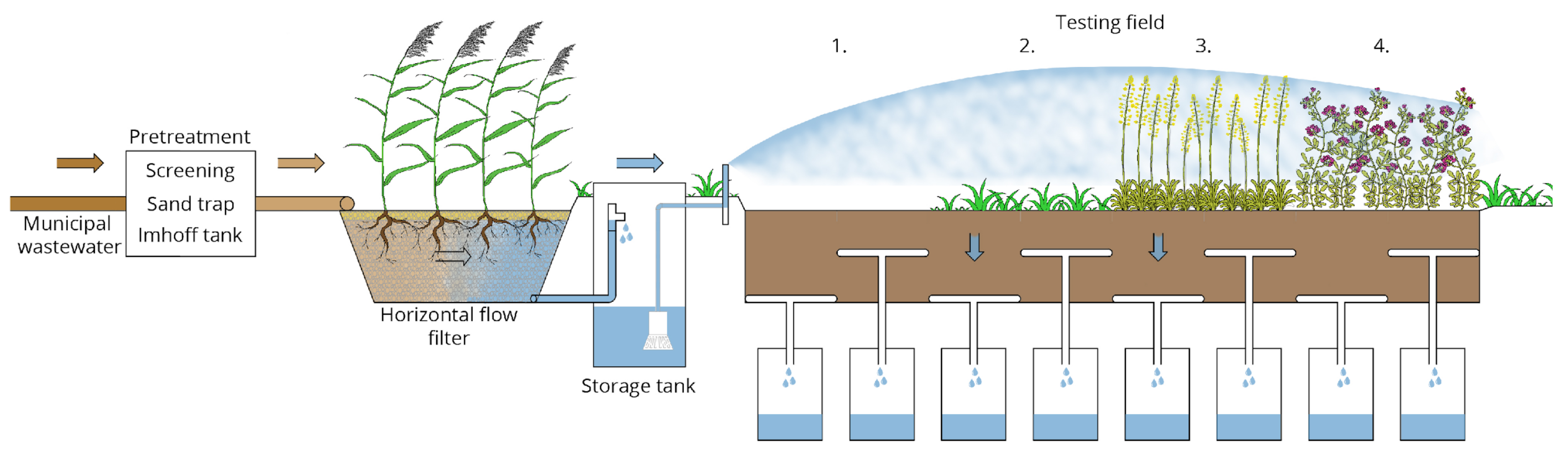
2.1. Site Description

The actual measurement was carried out at the multi-stage wastewater treatment plant for the municipality of Dražovice (850 EO). The municipality is situated in an agriculturally cultivated landscape, however, the area appears to be dry with insufficient rainfall for intensively cultivated agricultural land. The treatment plant is designed as an artificial wetland, whereby wastewater can be collected from any tributary/outfall within the series of connected stages. A sampling profile after a horizontally flowing filter with wetland plants was selected for measurement purposes. The filter itself exhibits low suspended solids concentrations, yet relatively high ammonia nitrogen concentrations. No mechanical treatment of the effluent was necessary for the measurements, the wastewater contains a minimum of suspended solids, so micro-spray irrigation is possible and there is no risk of clogging of the irrigation nozzle. The connection to the outflow of the horizontally flowing filter provides all-round favourable conditions for the connection of the irrigation system with the assumption of minimizing operational problems. Pollution concentrations at the outflow from the horizontal filter reach average values of 30.13 ± 11.73 mg/L for NH₄⁺-N and 3.909 ± 0.996 mg/L for TP. The applied effluent is first screened with coarse combs, then stripped of mineral material in a sand trap, followed by flow through a sedimentation tank and two parallel horizontal filters. A submersible pump is located in the inspection shaft behind the horizontal filter. The pump connection is deliberately chosen regardless of rainfall with a fixed mode throughout the measurement. The mode is set for 6 switches during the day, a daily water quantity of 15.5 mm/day was pumped to the test area. The pump was submerged below the level of the continuously flowing wastewater at all times (the average flow rate is 2.34 L/s), the supply pipe is fitted with a fine filter to prevent clogging of the irrigation sprinklers despite the minimum suspended solids. The pipeline to the irrigation units is laid at an almost non-freezing depth, and is only shallowly laid below ground level immediately before being brought above ground. The irrigation extension and directionally adjustable sprinkler units are directionally adjusted so that the irrigated area is sprayed as evenly as possible. Strong winds can be a negative factor, as the wind can carry small droplets of wastewater away from the intended irrigation area. For this reason, special nozzles with low spray height (approx. 40 cm) and larger droplet size were chosen. Therefore, this fact may have been neglected, and during irrigation, all irrigation water is considered as falling on the lysimeters.

2.2. Lysimeters Material

Soil samples were collected on homogenized material for annual consolidation at depths of 10, 30, 60, 80 and 100 cm with a 100 cm³ core auger. The saturated hydraulic conductivity was determined in the immediate vicinity of the lysimeters through a two-roll seepage test. The principle of the two-cylinder method consists in the central placement of two vertical cylinders in an intact earth body. The intensity of the seepage in the inner cylinder determines the saturated hydraulic conductivity after settling. The porosity of the material was determined on the intact samples, the value is determined by calculation according to the volume of the sample box and the weight of the dried sample. Two moisture contents were simultaneously determined on the samples at pressures of 33 and 1500 kPa (via a set of pressure chambers). At the same time, the sand (0.05–2.0 mm), clay (0.002–0.05 mm) contents (%) needed to be determined and these were carried out through sieve analysis on five disturbed samples. The clay (<0.002 mm) particle content was determined by the Cassagrande density method. The retention curve was determined using the inverse prediction function in Rosetta Lite v.1.1.US-1D [48]. The physical characteristics of the soil are given in

Table 1. Physical characteristics of soil layer in the field model.

Layer	Depth (cm)	θr (mm3/mm3)	θs (mm3/mm3)	α1 (1/mm)	n1	Ks (mm/day)	l
1	0–25	0.082	0.43	0.0021	1.317	60.1	0.5
2	25–45	0.081	0.435	0.0012	1.28	61.25	0.5
3	45–65	0.091	0.421	0.0017	1.249	57.44	0.5
4	65–85	0.097	0.423	0.0026	1.289	62.87	0.5
5	85–100	0.099	0.429	0.0024	1.299	59.84	0.5
Mean	0–100	0.09	0.428	0.002	1.287	60.3	0.5

θ_r—is the residual moisture content; θ_s—is the saturated moisture content; α₁—is the first coefficient of the macro domain; n₁—is the second coefficient of the macro domain; K_s—is the saturated conductivity; l—is the pore connectivity factor.

.

2.3. Experimental Design

The treated wastewater was used to irrigate a pre-treated area of 4.0 × 1.0 m with a surface that is aligned with the surrounding flat environment (Figure 1). Prior to the actual installation of the irrigation system, the soil horizon was exposed to a depth of 1.2 m and drainage pipes were installed at two depths. To ensure that sufficient water drained through the pipe, it was lined with a waterproofing impermeable foil in close proximity. The drainage was then backfilled with coarser 4/8 mm aggregate within 30 mm of the outer edge of the pipe. This was followed by a layer of up to 30 mm of washed sand as a transition filter. The follow-up material was the clay originally placed in the environment before the drainage was installed. The drainage pipe itself is followed by a drainage pipe to a sampling shaft located at a non-freezing depth. The side walls of the filtering environment are lined as closely as possible with hydro isolation. The leaking water cannot therefore flow unlimitedly within the vertical edge and only leaks downwards. Infiltration occurs naturally in an unsaturated soil environment. A saturated layer is not expected to form in the whole area for two reasons: the irrigation intensity is evenly distributed throughout the day and the drainage system drains water from the lower layers. However, as the model results show, the soil environment maintains a high moisture content, approaching near saturation. In practice, however, a very intense rainfall could result in a hydraulically saturated environment for a short period of time.

The vertical boundary condition is then a predefined type in the Hydrus environment: no-flux. The bottom settled layer can be defined as a seepage-face type boundary from the point of view of the Hydrus 2D numerical model development, which ensures that both moisture and pressure water move further unlimitedly. It was only in the deeper layer that the drainage pipe was laid, diverting all water to the intake profile in the inspection shaft. The whole area is divided into four sub-areas of 1.0 m² each, but connected. A 1.0 L sampling cup is fitted at the drainage pipe outlet in the sampling shaft area. A naturally cool environment is maintained in the shaft area regardless of the season. The effluent filtrate flows through the sampler respectively the excess water is retained in a larger container for the purpose of determining the volume of leakage. Water loss between sub-areas is neglected due to similar moisture conditions.

The surface of the test lysimeters is exposed to atmospheric conditions and is planted with M01—no vegetation, M02—grass mixture: 70% Perennial ryegrass (Lolium perenne), 10% meadowsweet (Poa pratensis), 20% red fescue (Festuca rubra), M03—oilseed rape (Brassica napus), M04—sown alfalfa (Medicago sativa). At the same time, an irrigation device is installed on the ground to ensure a constant inflow through the top edge for future numerical model definition. Thus, the upper edge receives pre-treated wastewater which is continuously diluted by rainfall. The volume of inflow is therefore not exactly constant, but is influenced by rainfall. Due to the use of the same and simultaneously homogenized filter material for all four lysimeters, the volumetric moisture contents at the beginning of the testing are also the same. The initial conditions are therefore identical for all models. Prior to the start of the measurements, the substrate was classified and the sand-clay-clay mixture ratio was determined, including the determination of the bulk density of the intact sample.

To find the hydraulic characteristics, we used the Hydrus 2D program, respectively, after finding two points of the retention curve and the volumetric mass, we used Rosetta lite to find all parameters entering the governing hydraulic equation of the numerical model: Q_r (mm³/mm³), Q_s (mm³/mm³), α₁ (1/mm), n₁, K_s (mm/day), l. The characteristics describing the model in the Hydrus 2D environment are given in

Table 2. Characteristics of the model in the Hydrus-2D environment.

Characteristics of the Model	Features, Description, Dimensions
Type of Geometry	2D—Vertical Plane XZ
Domain Definition	Rectangular (parametric) Lx = 500 mm, Lz = 1000 mm
Model discretization	0.050 mm
Main processes	Water flow, solute transport, root water uptake
Time discretization	Initial time step: 0.0001 day Minimum time step: 10–5 day Maximum time step: 5 days Final time: by specific in situ example
Initial condition	In the water content (uniform for the entire profile): Water content: 0.249
Inverse solution	Max. number of iteration: 10 Number of data points in the objective function: 15
Hydraulic model	Van Genuchten-Mualem No Hysteresis
Material characteristics	Mean values in the Table 1
Search reaction parameters for solute	Adsorption isotherm coefficient (Kd) First-order rate constant for dissolved phase (SinkWater1)
Number of time variable boundary conditions	15 conditions
Boundary condition	Upper boundary: atmospheric, third-type for solute transport Vertical boundary: no flux, without flow Lower boundary: seepage face

.

Since we have anticipated the use of Hydrus 2D, we have also adapted the lysimeters for the future boundary conditions in the numerical environment. The dimensions of the numerical model correspond to the dimensions of the 1:1 scale lysimeters. The lysimeters are strictly implemented with as much accuracy as possible (height 1000 mm, width 1000 mm and depth 1000 mm, drainage depths 500 and 1000 mm, drainage layer is 500 mm below the last extraction—this layer is not included in the model anymore). During the construction of the test lysimeters, we sampled the substrate used, then we determined the bulk density. Since we homogenized the substrate, we assume a uniform—equal—distribution of bulk moisture throughout the height. Regarding the initial condition related to the simulation of solute (NH₄⁺-N and TP) spreading, initial concentrations were not measured.

Prior to the measurements, the soil moisture was measured in the laboratory on substrate samples taken in the immediate vicinity of the lysimeters. Soil samples were collected in the laboratory environment, and 5 disturbed samples from different depths were verified by drying at 105 °C. The average soil moisture content, or initial condition for the numerical model, was 0.248 across the entire height (minor differences of up to 1% were neglected).

The research was based on experience gained in the previous phase of research work. Therefore, a nearly zero concentration (0.06 mg/L) of both monitored pollutants was assumed, although this hypothesis is not verified and introduces some error into the model.

2.4. Operational Conditions

Seepage face boundary condition was assigned to the bottom of the flow domain—water continues further into the bedrock, which is composed of the same material. An atmospheric boundary condition was assigned to the soil surface—in addition to precipitation, the boundary is loaded by evaporation and transpiration, which we do not separate, but instead unify into a single value describing the loss of water from the surface by evaporation.

Precipitation totals were measured at a distance of 100 m from the test area using a handheld ombrometer without time recording. Rainfall values were always considered for the previous period. If there was a situation where there was rainfall in the previous period in addition to irrigation with treated wastewater, we recalculated the pollution concentration. We considered atmospheric precipitation with minimal pollution (NH₄⁺-N and TP). The atmospheric boundary condition includes rainfall, evaporation for 2018, 2019, and 2020, and pollution concentration for 15, 13, and 13 records, respectively.

The amount of treated wastewater actually delivered was recorded by repeated measurements of the irrigation dose. The specific daily H_d dilute water load (rainfall) showed values of 14.50 ± 1.26 mm/day, 15.05 ± 1.20, 15.56 ± 0.67 and 16.0 ± 1.64 mm for the three measurement seasons, respectively, for the individual measurement campaigns.

As mentioned above, for the purpose of observing the spread of pollution, we used the easily detectable and most useful for practice pollutants: NH₄⁺-N and TP. We are aware of the complexity of the system when describing the environment in a complex way. There are numerous factors (bacteria, temperature, dissolved oxygen concentration, presence of organic pollution, anaerobic mass decomposition, etc.), yet our goal and effort is to produce a simplified model even at the cost of reducing the reliability of the numerical model. The average influent concentration of NH₄⁺-N in the treated wastewater is adjusted according to the rainfall intensity to (30.13 ± 11.73 mg/L) and 3.91 ± 0.97 mg/L for TP, respectively.

2.5. Sample Colection and Data Analysis

Water sampling was always carried out at intervals of 10–20 days for 211, 184 and 183 days in each year. The lysimeters were connected to the underground shaft through a drainage pipe so that it was easy to collect water samples from each sampling point. In the filtrate, we measured the amount of water (flow rate over the previous period). From the difference between inflow and outflow, we determined the actual evapotranspiration value (loaded error within the hydraulic storage of the soil profile). Pollution analysis was not performed on the entire accumulated amount (weekly volume), but on the sample that was mixed for a particular measurement day—even though the sample storage temperature was below 12 °C during the measurement. A sample of a few millilitres was analysed after collection by using a mobile photometric device. In the HYDRUS environment, the lower boundary of the area corresponded to a coarse seepage face type—the filter material goes on, the edge allowing the transfer of both moisture and pressurized water.

Eight filtrates, or one spilt water sample per day from each model, were collected for contamination analysis after flow through the soil profile. The lysimeters implemented their upper edge at approximately horizontal surrounding ground level, and to eliminate lateral runoff, the vertical walls were insulated with a thin waterproofing membrane. For this reason, there was no interaction between the individual models or the root systems of the plants present.

During the three years of measurements, measurements were carried out in extended growing seasons—so that we work in accordance with the current legislation, which allows the implementation of supplementary irrigation only in the growing season. In total, 41 sampling campaigns were carried out, and each sampling campaign analysed: the volume of total water filtered, determination of the volume of rainfall for the previous period on an ombrometer, conversion to evapotranspiration, sampling (inflow to lysimeters, outflow from eight lysimeters). For the calibration used to find the mathematically modelled environment describing the spread of NH₄⁺-N and TP pollution, we used 41 values of infiltrating water concentrations from each lysimeter. The reliability of the calibrated model was then assessed using Pearson’s coefficient of determination (R²), used to assess the level of compliance between predicted and observed pressure head data.

No equilibrium transport of solutes is involved in a sequential first-order decay reaction. Ammonium and phosphorus sorption and degradation is assumed to be a first-order kinetic rate process [38]. In this situation, it was considered strong simplification, without the influence of bacteria, dissolved oxygen, organic carbon and temperature. As reported by [38], the first-order rate constants may be used to represent a variety of reactions or transformations including biodegradation, volatilization and precipitation. The mass balance equation (1) when considering production and degradation is given by [49]:

$$\frac{\delta s_k^k}{\delta t}={\omega }_k\left[\left(1-f\right)\frac{k_{s,k}{c}_k^{{\beta }_k}}{1+{\eta }_k{c}_k^{{\beta }_k}}-s_k^k\right]-\left({\mu }_{s,k}+{\mu }_{s,k}^{\prime }\right)s_k^k+\left(1-f\right){\gamma }_{s,k}$$

(1)

Including the above simplifications, the modified equation is then formulated as:

$$\frac{\delta s_k^k}{\delta t}={\omega }_k\left[\left(1-f\right)k_{s,k}-s_k^k\right]$$

(2)

where:

• $s_k^k$—time-dependent sorption (g/g);
• t—time (day);
• ω_k—the first-order rate constant for the NH₄⁺-N (1/day);
• f—the fraction of exchange sites assumed to be in equilibrium with the solution phase;
• k_s,k—adsorption isotherm coefficient for material (mm³/μg);
• γ_s,k—zero-order rate constants for the solid (1/ML³/T);
• μ_s,k—first-order rate constants for solutes in the solid (1/T);
• β_k and ${\eta }_k$ (L³/M) are empirical coefficients.

3. Results

The basic idea of the results processing is to compare the simulation and the real measured values. At the same time, the measurements are not only based on a single experiment, but on three years of successive observations. In contrast to our previous lysimetric observation [41], the model calibration was performed only for the solute. While some of authors [50,51,52] in the HYDRUS-2D environment modified the model through calibration of hydraulic parameters, in this case, accurate laboratory determination of soil characteristics was used. The simplification of the model has a main objective: if in the future it is necessary to treat irrigation with wastewater in practice, the determination of soil characteristics at the laboratory scale is objectively faster than calibrating these characteristics through long-term in situ measurements and subsequent calibration in the numerical environment of the hydraulic model.

The filter material was implemented in the model based on laboratory analysis, or after determining the sand, clay and clay fractions, supplemented by the bulk mass of the intact sample. The calibration for the solute moving in the filter media consisted of finding the sorption parameters of this media in such a way that the nature of the media approximated the modelled infiltrating water concentrations as closely as possible to the actual measured values.

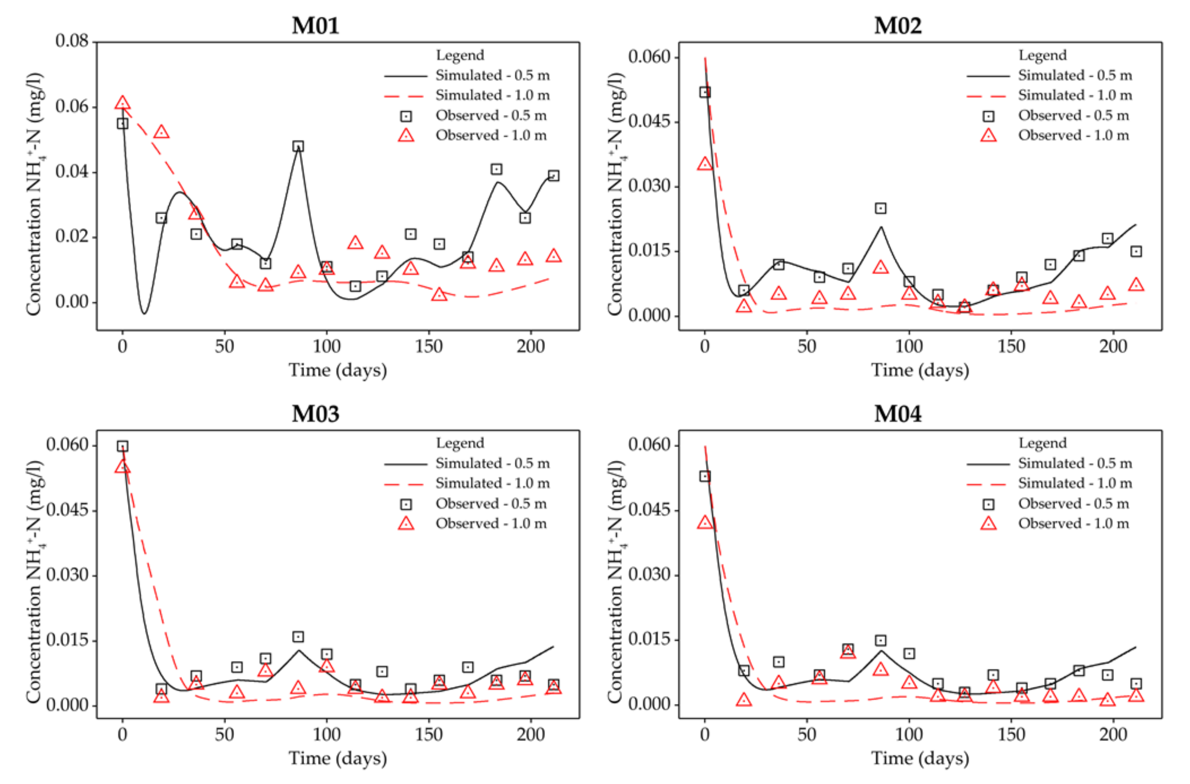
3.1. Ammonia Nitrogen

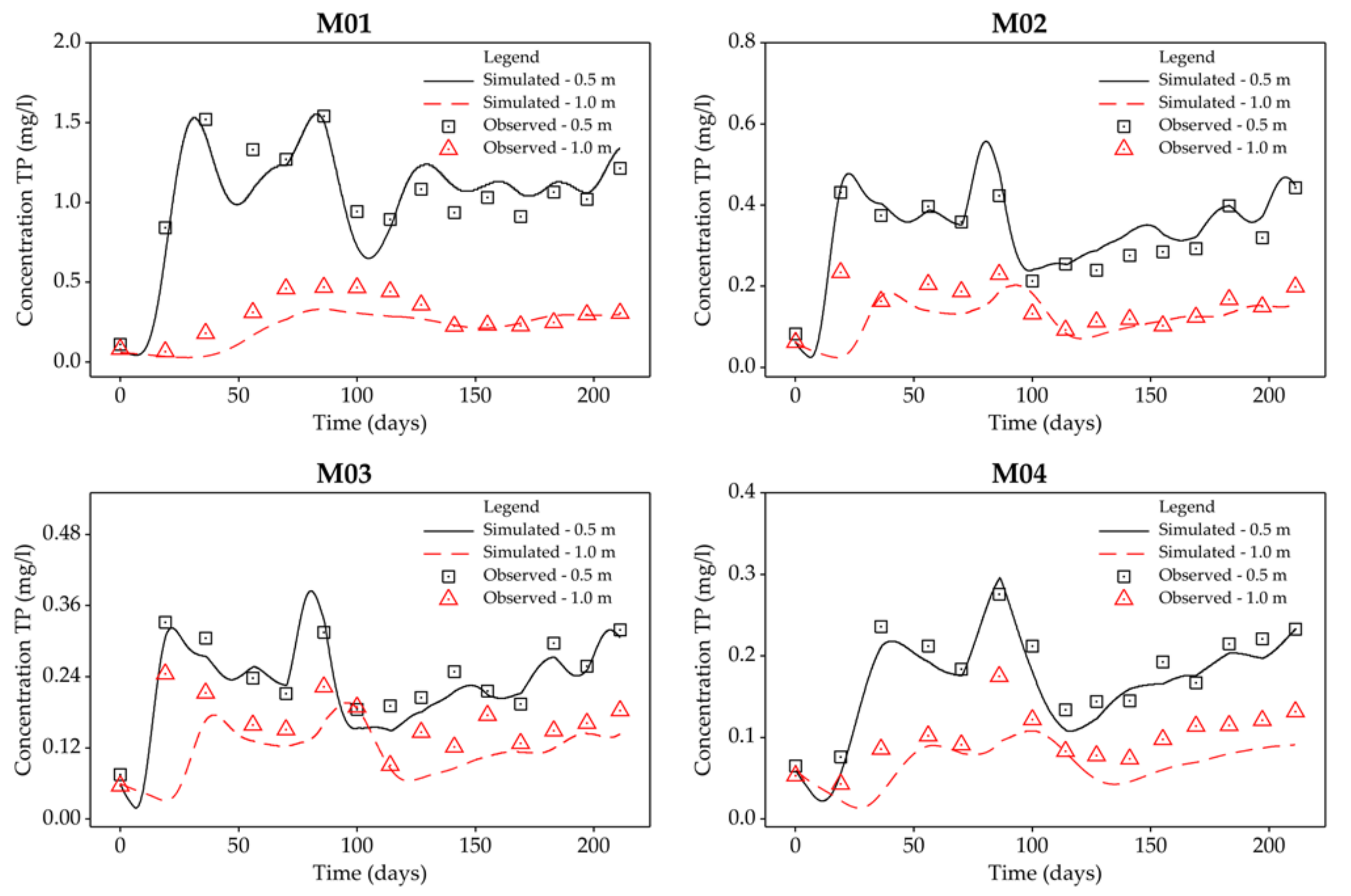
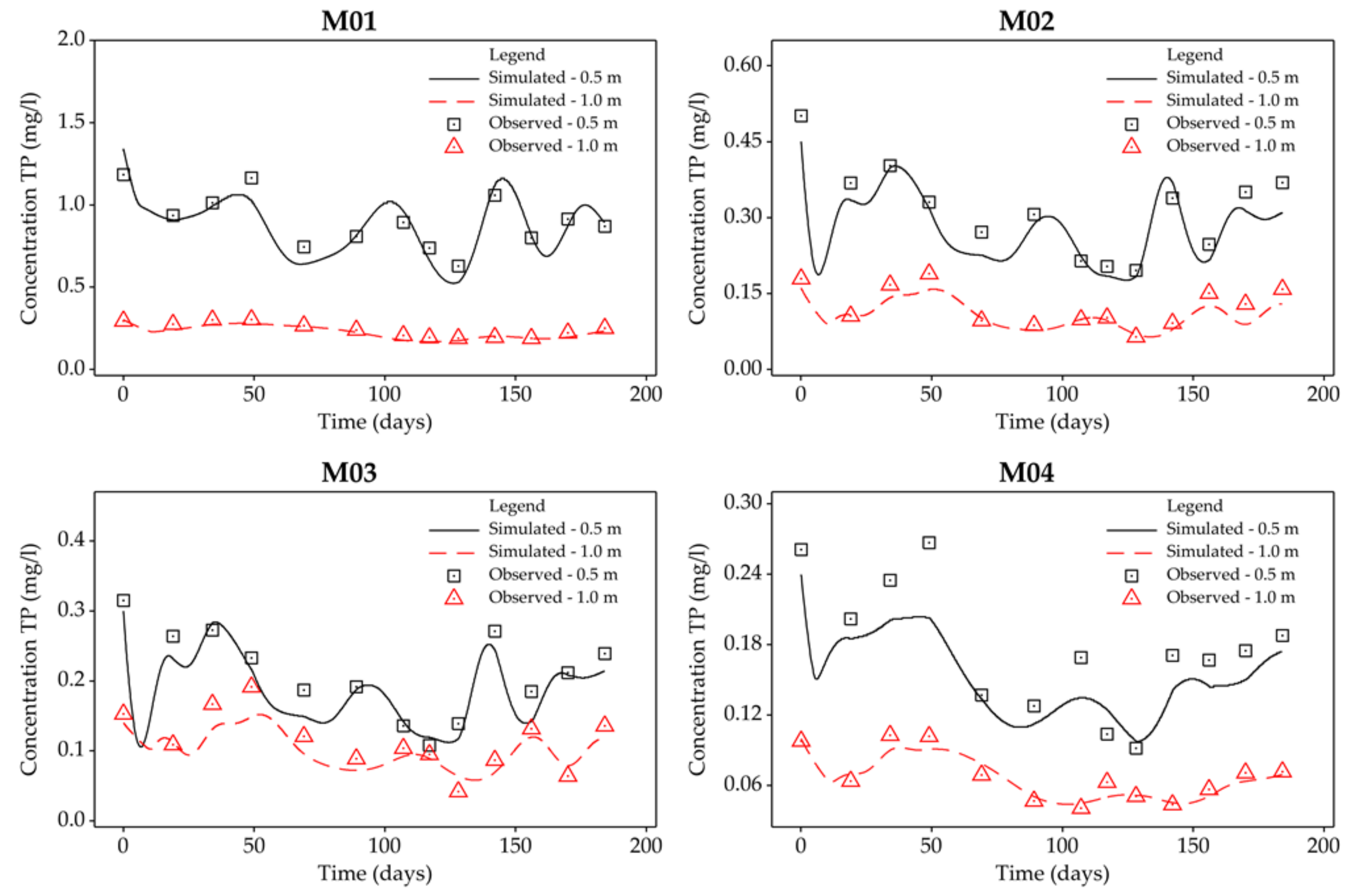
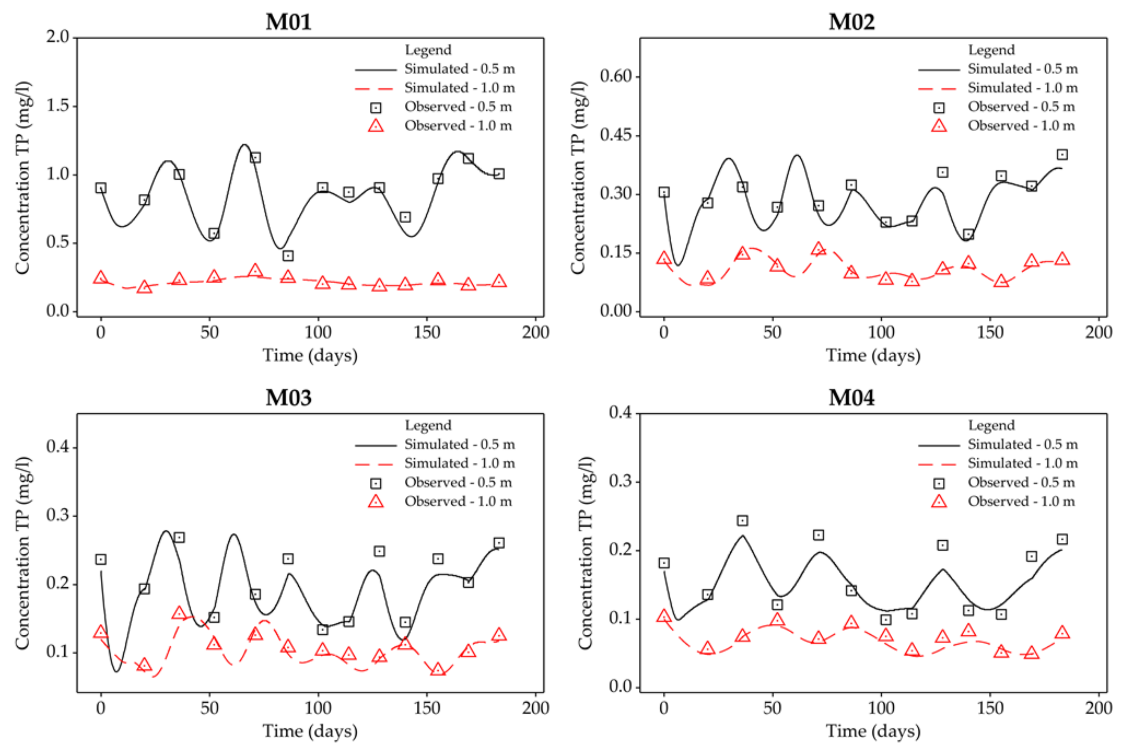
Before definitive excluding of the wastewater irrigation system, the contamination concentration in the soil profile (at various depths) is to be determined. The average input concentration in the three years was measured on a total of 41 samples as a value of 36.54 ± 11.95 mg/L. The pollution pattern in year 2018 is shown in Figure 2, year 2019 at Figure 3 and year 2020 at Figure 4. Due to exposure the pollution was diluted and the value was reduced to 30.13 ± 11.73 mg/L. The reduced value was determined by calculation based on the observed rainfall totals. All the infiltrating water concentrations for the four models are already reduced to harmless concentrations at 0.5 m depth. The observed concentrations, analysed in the laboratory, are 0.021 ± 0.011, 0.011 ± 0.008, 0.009 ± 0.009 and 0.009 ± 0.008 mg/L (

Table 3. Observed drainage NH₄⁺-N concentration (mg/L).

Variable	Depth (m)	n	Mean	SE Mean	StDev	Q1	Median	Q3
NH4+-N (A)	-	41	36.540	1.870	11.950	26.500	33.200	45.150
NH4+-N (B)	-	41	30.130	1.830	11.730	20.770	27.770	38.350
M01	0.5	41	0.021	0.002	0.011	0.012	0.018	0.027
	1.0	41	0.010	0.002	0.012	0.005	0.006	0.011
M02	0.5	41	0.011	0.001	0.008	0.006	0.010	0.014
	1.0	41	0.004	0.001	0.005	0.001	0.001	0.002
M03	0.5	41	0.009	0.001	0.009	0.005	0.007	0.010
	1.0	41	0.004	0.001	0.008	0.002	0.003	0.005
M04	0.5	41	0.009	0.001	0.008	0.005	0.007	0.011
	1.0	41	0.004	0.001	0.007	0.001	0.002	0.004

(A)—concentration in irrigation water, (B)—concentration after rainfall dilution, n—number of samples; SE Mean—standard error of the mean; StDev—standard deviation; Q₁ first quartile; Q₃—third quartile.

). At a depth of 1.0 m, the values are even lower, already at the limit of detectability up to 0.004 mg/L. A detailed evaluation is shown in Table 3. The results of the numerical model correspond to the measured values with a slight deviation. The evaluated results from approximately 4500–5300 simulated values for each model are also consistent with respect to satisfactory reliability. The average NH₄⁺-N pollution concentrations at 0.5 m depth for each model are 0.017 ± 0.011, 0.009 ± 0.005, 0.007 ± 0.005 and 0.007 ± 0.005 mg/L, followed by simulated values of 0.009 ± 0.011, 0.002 ± 0.004, 0.003 ± 0.006 and 0.002 ± 0.005 mg/L at 1.0 m depth (

Table 4. Simulated concentrations of NH₄⁺-N (mg/L).

Variable	Depth (m)	n	Mean	SE Mean	StDev	Q1	Median	Q3
M01	0.5	4582	0.017	0.000	0.011	0.008	0.014	0.025
	1.0	4582	0.009	0.000	0.011	0.004	0.006	0.007
M02	0.5	5256	0.009	0.000	0.005	0.005	0.008	0.012
	1.0	5256	0.002	0.000	0.004	0.001	0.001	0.002
M03	0.5	5376	0.007	0.000	0.005	0.004	0.006	0.010
	1.0	5376	0.003	0.000	0.006	0.001	0.002	0.003
M04	0.5	5221	0.007	0.000	0.005	0.004	0.006	0.009
	1.0	5221	0.002	0.000	0.005	0.001	0.001	0.002

n—number of samples; SE Mean—standard error of the mean; StDev—standard deviation; Q₁ first quartile; Q₃—third quartile.

).

3.2. TP Pollution

In the case of the TP contamination observations, the input concentrations are logically lower, averaging 4.76 ± 0.89 mg/L without dilution with rainwater and 3.91 ± 1.00 mg/L after dilution, respectively (

Table 5. Observed drainage TP concentration (mg/L).

Variable	Depth (m)	n	Mean	SE Mean	StDev	Q1	Median	Q3
TP (A)	-	41	4.762	0.139	0.893	4.005	4.760	5.417
TP (B)	-	41	3.909	0.156	0.996	3.177	3.957	4.633
M01	0.5	41	0.945	0.041	0.261	0.828	0.934	1.073
	1.0	41	0.251	0.014	0.089	0.193	0.231	0.295
M02	0.5	41	0.310	0.013	0.083	0.251	0.319	0.369
	1.0	41	0.130	0.007	0.044	0.097	0.123	0.160
M03	0.5	41	0.219	0.010	0.061	0.186	0.216	0.263
	1.0	41	0.129	0.007	0.045	0.096	0.125	0.158
M04	0.5	41	0.173	0.009	0.055	0.131	0.175	0.216
	1.0	41	0.081	0.004	0.028	0.057	0.075	0.100

(A)—concentration in irrigation water, (B)—concentration after rainfall dilution, n—number of samples; SE Mean—standard error of the mean; StDev—standard deviation; Q₁ first quartile; Q₃—third quartile.

). Infiltrating water concentrations at 0.5 m depth are reduced to 0.945 ± 0.261, 0.310 ± 0.083, 0.219 ± 0.061 and 0.173 ± 0.055 mg/L, respectively. The pollution pattern in year 2018 is shown in Figure 5, year 2019 at Figure 6 and year 2020 at Figure 7. Similar to NH₄⁺-N, the concentrations are reduced to 0.251 ± 0.089, 0.130 ± 0.044, 0.129 ± 0.045 and 0.081 ± 0.028 mg/L with increasing soil depth. The detailed evaluation is shown in Table 5. The results from the numerical model correlate again with the measured values. At a depth of 0.5 m, the observed numerical model values for each lysimeter are 0.922 ± 0.277, 0.306 ± 0.085, 0.205 ± 0.060 and 0.160 ± 0.044 mg/L. The depth of 1.0 m below the surface again shows better results, namely 0.215 ± 0.067, 0.112 ± 0.034, 0.106 ± 0.032 and 0.066 ± 0.019 (

Table 6. Simulated concentrations of TP (mg/L).

Variable	Depth (m)	n	Mean	SE Mean	StDev	Q1	Median	Q3
M01	0.5	5142	0.922	0.004	0.277	0.741	0.958	1.100
	1.0	5142	0.215	0.001	0.067	0.192	0.219	0.260
M02	0.5	5337	0.306	0.001	0.085	0.244	0.310	0.362
	1.0	5337	0.112	0.000	0.034	0.089	0.110	0.137
M03	0.5	5328	0.205	0.001	0.060	0.158	0.207	0.244
	1.0	5328	0.106	0.000	0.032	0.083	0.105	0.129
M04	0.5	5144	0.159	0.001	0.044	0.128	0.160	0.192
	1.0	5144	0.066	0.000	0.019	0.051	0.066	0.082

n—number of samples; SE Mean—standard error of the mean; StDev—standard deviation; Q₁ first quartile; Q₃—third quartile.

).

The setting of the initial condition probably introduces the largest error in the reliability of the model. We are aware of two major shortcomings in the model development—how to accurately determine the retained water content of the soil profile and how to determine the pollutant content of the entire observed profile. The “in situ” test environment was irrigated with clean (potable) water prior to actual wastewater application to stabilize the water content (th) of the entire profile. The resulting water content was determined by taking a disturbed sample and drying it at 105 °C in the laboratory. A total of 10 locations within all four lysimeters were sampled. Again, we note the difference between moisture content and retained water content. Nevertheless, we defined the initial value throughout the profile as th = 0.247. The initial pollution concentration was determined based on the infiltrating water concentration immediately prior to the start of wastewater application. Simulation in the numerical environment was only started at the time of initiation of wastewater irrigation, i.e., a delay of about 14 days. Simulated data followed the observed data and showed very good agreement in all displayed plots. As shown in the figures (Figure 5, Figure 6 and Figure 7), the coefficient of determination between measured pollution and simulation reached favourable values of 0.91, 0.95, 0.92 and 0.91 for NH₄⁺-N and values of 0.87, 0.92, 0.91 and 0.95 for TP for each model at 0.5 m depth during the first year of measurements (see more in

Table 7. Solute reaction parameters (k_s, ω_k) obtained by inverse solution for year 2018.

Variable	Depth (m)	NH4+-N			TP
		R2	ks (L/mg)	ωk (1/day)	R2	ks (L/mg)	ωk (1/day)
M01	0.5	0.91	0.16 × 10−1	0.490	0.87	7.33 × 10−2	0.100
	1.0	0.96	4.73 × 10−1	0.047	0.93	4.36 × 10−1	0.090
M02	0.5	0.95	4.37 × 10−1	0.524	0.92	3.13 × 10−5	0.172
	1.0	0.96	1.79 × 10−5	0.091	0.92	5.00 × 10−5	0.057
M03	0.5	0.92	9.26 × 10−1	0.538	0.91	2.83 × 10−5	0.197
	1.0	0.98	1.44 × 10−2	0.052	0.91	5.47 × 10−4	0.031
M04	0.5	0.91	9.13 × 10−1	0.540	0.95	2.40 × 10−1	0.212
	1.0	0.94	1.12 × 10−3	0.073	0.91	6.99 × 10−3	0.045

). In the downstream years, i.e., 2019 and 2020, the agreement values between the measured pollution and simulated concentrations are also satisfactory, with values for NH₄⁺-N in both years for 0.5 and 1.0 m depth ranging from 0.79 to 0.92 and 0.85 to 0.94 for TP, respectively. Detailed results are shown in

Table 8. Pearson’s coefficient of determination (R²) for years 2019 and 2020.

Variable	Depth (m)	NH4+-N		TP
		R2		R2
		2019	2020	2019	2020
M01	0.5	0.90	0.86	0.88	0.93
	1.0	0.91	0.79	0.90	0.86
M02	0.5	0.91	0.89	0.92	0.91
	1.0	0.90	0.88	0.89	0.88
M03	0.5	0.92	0.91	0.91	0.91
	1.0	0.86	0.87	0.88	0.85
M04	0.5	0.91	0.91	0.90	0.94
	1.0	0.86	0.87	0.88	0.88

.

As other results show [46], it is clearly demonstrated the importance of irrigation in the period of year with high evapotranspiration values and low rainfall. This rule applies in the case of irrigation with clean water. If it is necessary to irrigate using another source, it is necessary to comply with additional safety requirements.

4. Discussion

Groundwater recharge with treated municipal wastewater presents a wide range of technical and health issues that need to be carefully evaluated before implementation at operational scale [53]. While the authors [54] found that treated effluent discharge can consume oxygen in soil layers when applying the Managed Aquifer Recharge (MAR) method, the oxygen and ammonia-nitrogen balance is quite balanced in the case of controlled and gradual irrigation. That is, if the soil layer is not hydraulically overloaded, there is no need for a water-saturated environment and ammonia nitrogen is able to successfully convert to nitrate. The fundamental difference in ammonia removal efficiency also lies in the organic material content of the soil. When soils with a high organic substrate content are oversaturated, the reaction between nitrate and organic material results in the production of ammoniacal nitrogen. This means that soils with a low organic matter content and an unsaturated soil profile are not at risk of ammonia production, as confirmed by the authors [55]. Effective ammonia removal in permeable filter media can be observed with expectation for sand filters. Examples include up to 92% efficiency in the summer season [56], or the inlet concentration of 39 mg/L being reduced to 2.4 mg/L at a depth of 150 cm. Irrigation with pre-treated wastewater proved to be effective in our case as well. Optimizing the irrigation rate and keeping it in the unsaturated zone resulted in an efficiency of up to 99.98%, or a reduction of the influent concentration of 36.54 mg/L to 0.004 mg/L at a depth of 1.0 m.

In addition to the effective removal of ammonia nitrogen, wastewater irrigation brings effective removal of faecal pollution when properly set up. Authors [57,58] found a temperature dependence of ammonia removal efficiency. Given the assumption of applying irrigation only during the growing season, temperatures below 2 °C cannot be assumed, therefore the reduction in ammonia removal efficiency or the risk of bacterial contamination should not be significant. Authors of similar studies have monitored the dependence of the nitrification process near the surface with a temperature optimum at 35 °C and a decrease in efficiency below 20 °C [59,60]. At the same time, the type of irrigation (drip irrigation or furrow irrigation) has been found to affect the activity of nitrifying bacteria [61] and nitrification, respectively [62,63]. In comparison with our research and the high ammonia removal efficiency (99.7%) already found at a depth of 50 cm below the surface, we assume that the regular irrigation by spraying in several daily cycles was just creating an optimal environment to ensure nitrification. Regarding the mobility of ammoniacal nitrogen, similar to the authors [64] or [58], we did not identify ammoniacal nitrogen mobility to deeper layers. This was most likely due to the minimal presence of organic matter both in the environment itself and in the influent wastewater. At the same time, there was also a sufficient amount of sandy mineral particles in the soil, which, according to these authors, are a prerequisite for the suppression of ammonia mobility.

The above-mentioned context points to the fact that we can quite reliably ensure the minimisation of ammonia transport to groundwater—but only if the optimum operating conditions are strictly observed. However, it should be noted that the nitrate load reaching groundwater is not reduced. On the contrary, nitrification processes are increasing their concentration.

The above results show that it is possible to minimise ammonia transport to groundwater with the correct input parameters and under appropriate operating conditions.

As in the case of ammonia nitrogen, a significant reduction in TP concentration can be observed in the course of infiltration through the soil profile. From the measured values, it is possible to reveal the dependence of the output concentration on the depth of the soil layer, as evidenced by the results of the authors [56]. In their study, the PO₄-P removal efficiency averaged around 64% for a daily hydraulic load of 0.27 m³/m² and 63% for a hydraulic load of 0.40 m³/m². At the same time, the different and considerably higher influent concentrations, which reached up to 29.1 mg/L PO₄-P in the case of these authors, should be taken into account. The filter bed, sand bed and sampling depth of 1.5 m were also different. Compared to our study, in which TP removal efficiencies reached up to 97%, the compared results represent significantly lower efficiencies. Similarly, lower TP removal efficiencies are also evidenced by a study [65] in which runoff concentrations of 6.7 mg/L were achieved at a depth of 0.8 m (inflow concentrations averaged 8.67 mg/L) when using sand ground filters. The relationship between hydraulic loading and outflow PO₄-P concentrations was described by the authors [66] where at least 50% PO₄-P removal efficiency was observed at a depth of 1.5 m despite increasing hydraulic loading. The authors report that no saturation of the soil profile was observed during the application of intense rainfall, which would reduce the efficiency of the ongoing biochemical reactions, which corresponds with our measurements. However, the authors point out that transport of remaining PO₄-P into streams and lakes by groundwater cannot be ruled out, which may cause the greatest ecological risk—eutrophication of standing water. We can agree with this statement because despite almost 97% TP removal efficiency, the average runoff concentration at 1.0 m depth was 0.15 mg/L TP. An unresolved issue is the further evolution and transport of TP in the soil environment. Numerical modelling is a suitable tool for this purpose and provides at least a rough estimate of the evolution in the soil horizon.

The issue of nutrient transport to groundwater is often associated with the use of Vegetative Filter Strips (VFS)—grassed strips within agricultural areas. The amount of TP removed is often linked to the dimensions of the VFS itself, particularly the depth. Significant TP reduction when a VFS of 1.2 m depth penetrates the soil layer is documented by [67], where efficiencies of up to 70% have been recorded. It offers the possibility and use of phosphorus elimination through a combination of VFS and irrigation with treated wastewater. In this case, VFS could provide an insurance mechanism to suppress the risk of phosphorus transport to groundwater or reservoirs.

Wastewater irrigation does not only affect the groundwater or soil profile, but also the vegetation on the surface. The authors of [68,69] reported significant differences in biomass production when irrigating lettuce with wastewater compared to irrigation with potable water. This involves an increase in nutrient content in both above and below ground plant parts leading to increased lettuce production. The differences in runoff TP concentrations within columns M01–M04 can be attributed to the utilization of nutrients, mainly phosphorus, by plants at the surface. The highest efficiency in phosphorus removal is achieved by the M04—sown alfalfa (Medicago sativa) body, where the runoff concentration averages 0.17 mg/L and 0.08 mg/L for depths of 0.5 m and 1.0 m, respectively.

5. Conclusions

In order to follow the evolution of the solution distribution in the soil profile, two basic mathematical models were created using Hydrus 2D software. A model describing the distribution of ammoniacal nitrogen distribution and a similar model for monitoring the progress of total phosphorus during filtration in the soil environment. The models have been deliberately simplified into the most accessible version possible, without including the biochemistry-based processes. We have completely suppressed bacterial activity, the presence of oxygen, the presence and uptake of organic substrate, other forms of nitrogen, temperature and other properties, including calibrating the model based on the observed physical characteristics of the material.

For the research, lysimeter experiments were set up near an artificial wetland, with irrigation water stripped of most suspended solids to eliminate clogging problems in the irrigation system. The tested columns were loaded with an average rate of 15.5 mm/day and concentrations of 30.1 mg/L ammoniacal nitrogen and 3.9 mg/L total phosphorus, respectively—values corresponding, for example, to a poorly functioning outfall from a wastewater treatment plant in the Czech Republic.

Subsequently, numerical models were developed to match the operation of the test lysimeters (M01 to M04). The physical properties of the soil material were implemented in the models without further calibration. The calibration itself focused on the determination of characteristics describing the change in solution concentration during filtration in porous media. The values of k_s and ω_k were determined for each model and solution separately. In particular, the aim was to objectively assess the reliability of the R² model.

When the numerical model was built in 2018, R² values after calibration ranged from 0.91 to 0.98 for NH₄⁺-N and 0.87 to 0.95 for TP. Satisfactory reliabilities were also found in the follow-up years 2019 and 2020, when the models were verified and compared with real leachates. Despite the significant simplification, R² values are = 0.90 and 0.87 in 2019 and 2020 for NH₄⁺-N and TP pollution, respectively. For TP pollution, R² values are = 0.90 in both years. A slight deterioration can be observed when looking at the effect of depth on model reliability. On average, the reliability is always worse for all four models, with a 1.0 m depth resulting in a 1–5% deterioration compared to the 0.5 m depth.

Regarding the evolution of pollution along the height of the profile, NH₄⁺-N concentrations were close to zero already at 0.5 m depth without any significant dependence on the type of irrigated vegetation. It is necessary to state that the surface was loaded with wastewater so that saturation of the aquatic environment never occurred. The average daily ammoniacal nitrogen application rate of 0.467 g/m²/day was significantly higher than what the cultivated crop is able to use.

In contrast, elevated TP concentrations were observed down to a depth of 1.0 m below ground level. As expected, the reduction in pollution was lower than for ammoniacal nitrogen. The reduction of TP concentration in infiltrating water depended more strongly on the type of vegetation used than in the case of NH₄⁺-N. Test columns planted with oilseed rape (Brassica napus) and alfalfa (Medicago sativa) showed the lowest values of concentrations in the runoff. Increased TP concentrations in the soil profile may ensure the availability of phosphorus for vegetation species that root deeper below the surface, typically to a depth of 0.8 m. Conversely, ammoniacal nitrogen is likely transformed to nitrate nitrogen immediately in the subsurface. From the point of view of the issue of ammonia diffusion to groundwater, ammonia nitrogen may not be a problem, but the operation of the soil environment under aerobic conditions must always be observed.

However, the complexity and intricacy of the description of the system in wastewater irrigation does not predetermine this practice for wastewater disposal in a global perspective. Health risks, hygienic environment, pharmaceuticals in wastewater, heavy metal loading, soil salinization, etc., are factors that cannot be ignored. This has not been evaluated in the paper and should be the subject of further research.

References

1. The State of Food and Agriculture 2020: Overcoming Water Challenges in Agriculture; FAO: Rome, Italy, 2020; ISBN 978-92-5-133441-6.
2. The State of Food and Agriculture: Investing in Agriculture for a Better Future; FAO: Rome, Italy, 2012; ISBN 978-92-5-107317-9.
3. The State of Food and Agriculture 2018: Migration, Agriculture and Rural Development; FAO: Rome, Italy, 2018; ISBN 978-92-5-130568-3.
4. Feyen, L.; Ciscar Martinez, J.; Gosling, S.; Ibarreta Ruiz, D.; Soria Ramirez, A.; Dosio, A.; Naumann, G.; Russo, S.; Formetta, G. Climate Change Impacts and Adaptation in Europe; Publications Office of the European Union: Luxembourg, 2020; ISBN 978-92-76-18123-1. [Google Scholar]
5. Bocci, M.; Smanis, T. Assessment of the Impacts of Climate Change on the Agriculture Sector in the Southern Mediterranean: Foreseen Developments and Policy Measures; Union for the Mediterranean: Barcelona, Spain, 2019. [Google Scholar]
6. The European Environment—State and Outlook 2020: Executive Summary; European Environment Agency: Copenhagen, Denmark, 2019; ISBN 978-92-9480-115-9.
7. Jacobs, C.; Berglund, M.; Kurnik, B.; Dworak, T.; Marras, S.; Mereu, V.; Michetti, M. Climate Change Adaptation in the Agriculture Sector in Europe; European Environment Agency: København, Denmark, 2019. [Google Scholar]
8. Wriedt, G.; Van der Velde, M.; Aloe, A.; Bouraoui, F. Estimating irrigation water requirements in Europe. J. Hydrol. 2009, 373, 527–544. [Google Scholar] [CrossRef]
9. Wichelns, D. Achieving Water and Food Security in 2050: Outlook, Policies, and Investments. Agriculture 2015, 5, 188–220. [Google Scholar] [CrossRef] [Green Version]
10. Council Directive 91/271/EEC of 21 May 1991 Concerning Urban Waste-Water Treatment. Available online: https://eur-lex.europa.eu/eli/dir/1991/271/oj (accessed on 20 August 2021).
11. Toze, S. Reuse of effluent water—Benefits and risks. Agric. Water Manag. 2006, 80, 147–159. [Google Scholar] [CrossRef] [Green Version]
12. Bixio, D.; Thoeye, C.; De Koning, J.; Joksimovic, D.; Savic, D.; Wintgens, T.; Melin, T. Wastewater reuse in Europe. Desalination 2006, 187, 89–101. [Google Scholar] [CrossRef]
13. Almeelbi, T.; Ismail, I.; Basahi, J.; Qari, H.; Hassan, I. Hazardous of Waste Water Irrigation on Quality Attributes and Contamination of Citrus Fruits. Biosci. Biotechnol. Res. Asia 2014, 11, 89–97. [Google Scholar] [CrossRef]
14. Zhang, J. Barriers to water markets in the Heihe River basin in northwest China. Agric. Water Manag. 2007, 87, 32–40. [Google Scholar] [CrossRef]
15. Ors, S.; Turan, M.; Kiziloglu, F.; Sahin, U.; Esringu, A. Evaluation of Long-Term Waste Water Irrigation on Chemical Properties of Soil and Barley Undergrowth Field Conditions. In Proceedings of the International Sustainable Water and Wastewater Management Symposium Proceedings, Konya, Turkey, 26–28 October 2010; pp. 1179–1189. [Google Scholar]
16. Sasani, F.; Ghamarnia, H.; Yargholi, B. Assessment of long term wastewater irrigation impacts on spatial distribution of salinity and sodicity parameters. Water Irrig. Manag. 2015, 5, 229–241. [Google Scholar]
17. Zikalala, P.; Kisekka, I.; Grismer, M. Calibration and Global Sensitivity Analysis for a Salinity Model Used in Evaluating Fields Irrigated with Treated Wastewater in the Salinas Valley. Agriculture 2019, 9, 31. [Google Scholar] [CrossRef] [Green Version]
18. Colon, B.; Toor, G. A Review of Uptake and Translocation of Pharmaceuticals and Personal Care Products by Food Crops Irrigated with Treated Wastewater. In Advances in Agronomy; Elsevier: Amsterdam, The Netherlands, 2016; pp. 75–100. ISBN 9780128046913. [Google Scholar]
19. De Jong, R.; Drury, C.; Yang, J.; Campbell, C. Risk of water contamination by nitrogen in Canada as estimated by the IROWC-N model. J. Environ. Manag. 2009, 90, 3169–3181. [Google Scholar] [CrossRef]
20. Korsaeth, A.; Eltun, R. Nitrogen mass balances in conventional, integrated and ecological cropping systems and the relationship between balance calculations and nitrogen runoff in an 8-year field experiment in Norway. Agric. Ecosyst. Environ. 2000, 79, 199–214. [Google Scholar] [CrossRef]
21. Yang, X.; Lu, Y.; Tong, Y.; Yin, X. A 5-year lysimeter monitoring of nitrate leaching from wheat–maize rotation system: Comparison between optimum N fertilization and conventional farmer N fertilization. Agric. Ecosyst. Environ. 2015, 199, 34–42. [Google Scholar] [CrossRef]
22. Wick, K.; Heumesser, C.; Schmid, E. Groundwater nitrate contamination: Factors and indicators. J. Environ. Manag. 2012, 111, 178–186. [Google Scholar] [CrossRef] [Green Version]
23. Groenveld, T.; Argaman, A.; Šimůnek, J.; Lazarovitch, N. Numerical modeling to optimize nitrogen fertigation with consideration of transient drought and nitrogen stress. Agric. Water Manag. 2021, 254, 106971. [Google Scholar] [CrossRef]
24. Azad, N.; Behmanesh, J.; Rezaverdinejad, V.; Abbasi, F.; Navabian, M. An analysis of optimal fertigation implications in different soils on reducing environmental impacts of agricultural nitrate leaching. Sci. Rep. 2020, 10, 1–15. [Google Scholar] [CrossRef] [PubMed]
25. Elgallal, M.; Fletcher, L.; Evans, B. Assessment of potential risks associated with chemicals in wastewater used for irrigation in arid and semiarid zones: A review. Agric. Water Manag. 2016, 177, 419–431. [Google Scholar] [CrossRef]
26. Paul, M.; Negahban-Azar, M.; Shirmohammadi, A.; Montas, H. Developing a Multicriteria Decision Analysis Framework to Evaluate Reclaimed Wastewater Use for Agricultural Irrigation: The Case Study of Maryland. Hydrology 2021, 8, 4. [Google Scholar] [CrossRef]
27. Li, L.; Duan, M.; Fu, H. Supporter Profiling in Recycled Water Reuse: Evidence from Meta-Analysis. Water 2020, 12, 2735. [Google Scholar] [CrossRef]
28. Schwaller, C.; Keller, Y.; Helmreich, B.; Drewes, J. Estimating the agricultural irrigation demand for planning of non-potable water reuse projects. Agric. Water Manag. 2021, 244, 106529. [Google Scholar] [CrossRef]
29. Shoushtarian, F.; Negahban-Azar, M. Worldwide Regulations and Guidelines for Agricultural Water Reuse: A Critical Review. Water 2020, 12, 971. [Google Scholar] [CrossRef] [Green Version]
30. Rizzo, L.; Krätke, R.; Linders, J.; Scott, M.; Vighi, M.; de Voogt, P. Proposed EU minimum quality requirements for water reuse in agricultural irrigation and aquifer recharge: SCHEER scientific advice. Curr. Opin. Environ. Sci. Health 2018, 2, 7–11. [Google Scholar] [CrossRef]
31. Sánchez-Cerdà, C.; Salgot, M.; Folch, M. Reuse of reclaimed water: What is the direction of its evolution from a European perspective? In Wastewater Treatment and Reuse—Present and Future Perspectives in Technological Developments and Management Issues; Advances in Chemical Pollution, Environmental Management and Protection; Elsevier: Amsterdam, The Netherlands, 2020; pp. 1–64. ISBN 9780128201701. [Google Scholar]
32. Russo, D.; Zaidel, J.; Fiori, A.; Laufer, A. Numerical analysis of flow and transport from a multiple-source system in a partially saturated heterogeneous soil under cropped conditions. Water Resour. Res. 2006, 42. [Google Scholar] [CrossRef]
33. Russo, D.; Laufer, A.; Bar-Tal, A. Improving water uptake by trees planted on a clayey soil and irrigated with low-quality water by various management means: A numerical study. Agric. Water Manag. 2020, 229, 105891. [Google Scholar] [CrossRef]
34. Grecco, K.; Miranda, J.; Silveira, L.; van Genuchten, M. HYDRUS-2D simulations of water and potassium movement in drip irrigated tropical soil container cultivated with sugarcane. Agric. Water Manag. 2019, 221, 334–347. [Google Scholar] [CrossRef]
35. Yin, H.; Xu, Z.; Li, H.; Li, S. Numerical Modeling of Wastewater Transport and Degradation in Soil Aquifer. J. Hydrodyn. 2006, 18, 597–605. [Google Scholar] [CrossRef]
36. Tournebize, J.; Gregoire, C.; Coupe, R.; Ackerer, P. Modelling nitrate transport under row intercropping system: Vines and grass cover. J. Hydrol. 2012, 440–441, 14–25. [Google Scholar] [CrossRef]
37. Wei, X.; Bailey, R.; Records, R.; Wible, T.; Arabi, M. Comprehensive simulation of nitrate transport in coupled surface-subsurface hydrologic systems using the linked SWAT-MODFLOW-RT3D model. Environ. Model. Softw. 2019, 122, 104242. [Google Scholar] [CrossRef]
38. Simunek, J.; van Genuchten, M.; Sejna, M. The HYDRUS Software Package for Simulating Two- and Three- Dimensional Movement of Water, Heat, and Multiple Solutes in Variably-Saturated Media; Technical Manual, Version 2.0; PC Progress: Prague, Czech Republic, 2011. [Google Scholar]
39. Yao, F.; Huang, J.; Cui, K.; Nie, L.; Xiang, J.; Liu, X.; Wu, W.; Chen, M.; Peng, S. Agronomic performance of high-yielding rice variety grown under alternate wetting and drying irrigation. Field Crops Res. 2012, 126, 16–22. [Google Scholar] [CrossRef]
40. Askar, M.; Youssef, M.; Chescheir, G.; Negm, L.; King, K.; Hesterberg, D.; Amoozegar, A.; Skaggs, R. DRAINMOD Simulation of macropore flow at subsurface drained agricultural fields: Model modification and field testing. Agric. Water Manag. 2020, 242, 16–22. [Google Scholar] [CrossRef]
41. Kriška, M.; Němcová, M.; Hyánková, E. The influence of ammonia on groundwater quality during wastewater irrigation. Soil Water Res. 2018, 13, 161–169. [Google Scholar]
42. Dong, Y.; Safferman, S.; Nejadhashemi, A. Land-Based Wastewater Treatment System Modeling Using HYDRUS CW2D to Simulate the Fate, Transport, and Transformation of Soil Contaminants. J. Sustain. Water Built Environ. 2019, 5, 04019005. [Google Scholar] [CrossRef]
43. Parihar, C.; Nayak, H.; Rai, V.; Jat, S.; Parihar, N.; Aggarwal, P.; Mishra, A. Soil water dynamics, water productivity and radiation use efficiency of maize under multi-year conservation agriculture during contrasting rainfall events. Field Crops Res. 2019, 241, 107570. [Google Scholar] [CrossRef]
44. Iqbal, S.; Guber, A.; Khan, H. Estimating nitrogen leaching losses after compost application in furrow irrigated soils of Pakistan using HYDRUS-2D software. Agric. Water Manag. 2016, 168, 85–95. [Google Scholar] [CrossRef]
45. Šimunek, J.; van Genuchten, M.; Šejna, M. HYDRUS: Model Use, Calibration, and Validation. Trans. ASABE 2012, 55, 1261–1274. [Google Scholar]
46. Marković, M.; Filipović, V.; Legović, T.; Josipović, M.; Tadić, V. Evaluation of different soil water potential by field capacity threshold in combination with a triggered irrigation module. Soil Water Res. 2015, 10, 164–171. [Google Scholar] [CrossRef] [Green Version]
47. Pan, X.; Lv, J.; Dyck, M.; He, H. Bibliometric Analysis of Soil Nutrient Research between 1992 and 2020. Agriculture 2021, 11, 223. [Google Scholar] [CrossRef]
48. Schaap, M.; Leij, F.; van Genuchten, M. Rosetta: A computer program for estimating soil hydraulic parameters with hierarchical pedotransfer functions. J. Hydrol. 2001, 251, 163–176. [Google Scholar] [CrossRef]
49. Toride, N.; Leij, F.; van Genuchten, M. A comprehensive set of analytical solutions for nonequilibrium solute transport with first-order decay and zero-order production. Water Resour. Res. 1993, 29, 2167–2182. [Google Scholar] [CrossRef]
50. Sakaguchi, A.; Yanai, Y.; Sasaki, H. Subsurface irrigation system design for vegetable production using HYDRUS-2D. Agric. Water Manag. 2019, 219, 12–18. [Google Scholar] [CrossRef]
51. Karandish, F.; Šimůnek, J. A comparison of the HYDRUS (2D/3D) and SALTMED models to investigate the influence of various water-saving irrigation strategies on the maize water footprint. Agric. Water Manag. 2019, 213, 809–820. [Google Scholar] [CrossRef] [Green Version]
52. Shan, G.; Sun, Y.; Zhou, H.; Schulze Lammers, P.; Grantz, D.; Xue, X.; Wang, Z. A horizontal mobile dielectric sensor to assess dynamic soil water content and flows: Direct measurements under drip irrigation compared with HYDRUS-2D model simulation. Biosyst. Eng. 2019, 179, 13–21. [Google Scholar] [CrossRef]
53. Asano, T.; Cotruvo, J. Groundwater recharge with reclaimed municipal wastewater: Health and regulatory considerations. Water Res. 2004, 38, 1941–1951. [Google Scholar] [CrossRef]
54. Silver, M.; Knöller, K.; Schlögl, J.; Kübeck, C.; Schüth, C. Nitrogen cycling and origin of ammonium during infiltration of treated wastewater for managed aquifer recharge. Appl. Geochem. 2018, 97, 71–80. [Google Scholar] [CrossRef]
55. Reemtsma, T.; Gnirß, R.; Jekel, M. Infiltration of combined sewer overflow and tertiary municipal wastewater: An integrated laboratory and field study on nutrients and dissolved organics. Water Res. 2000, 34, 1179–1186. [Google Scholar] [CrossRef]
56. Bali, M.; Gueddari, M. Removal of phosphorus from secondary effluents using infiltration–percolation process. Appl. Water Sci. 2019, 9, 54. [Google Scholar] [CrossRef] [Green Version]
57. Ausland, G.; Stevik, T.; Hanssen, J.; Køhler, J.; Jenssen, P. Intermittent filtration of wastewater—Removal of fecal coliforms and fecal streptococci. Water Res. 2002, 36, 3507–3516. [Google Scholar] [CrossRef]
58. Chilundo, M.; Joel, A.; Wesström, I.; Brito, R.; Messing, I. Influence of irrigation and fertilisation management on the seasonal distribution of water and nitrogen in a semi-arid loamy sandy soil. Agric. Water Manag. 2018, 199, 120–137. [Google Scholar] [CrossRef]
59. Myers, R. Temperature effects on ammonification and nitrification in a tropical soil. Soil Biol. Biochem. 1975, 7, 83–86. [Google Scholar] [CrossRef]
60. Lees, H.; Quastel, J. Biochemistry of nitrification in soil: 3. Nitrification of various organic nitrogen compounds. Biochem. J. 1946, 40, 824–828. [Google Scholar] [CrossRef] [Green Version]
61. Aulakh, M.; Singh, K.; Singh, B.; Doran, J. Kinetics of nitrification under upland and flooded soils of varying texture. Commun. Soil Sci. Plant Anal. 2008, 27, 2079–2089. [Google Scholar] [CrossRef]
62. Thorburn, P.; Cook, F.; Bristow, K. Soil-dependent wetting from trickle emitters: Implications for system design and management. Irrig. Sci. 2003, 22, 121–127. [Google Scholar] [CrossRef]
63. Thorburn, P.; Dart, I.; Biggs, I.; Baillie, C.; Smith, M.; Keating, B. The fate of nitrogen applied to sugarcane by trickle irrigation. Irrig. Sci. 2003, 22, 201–209. [Google Scholar] [CrossRef]
64. Omar, L.; Ahmed, O.; Majid, N. Improving Ammonium and Nitrate Release from Urea Using Clinoptilolite Zeolite and Compost Produced from Agricultural Wastes. Sci. World J. 2015, 2015, 574201. [Google Scholar] [CrossRef]
65. Kholoma, E.; Renman, G.; Renman, A. Phosphorus removal from wastewater by field-scale fortified filter beds during a one-year study. Environ. Technol. 2016, 37, 2953–2963. [Google Scholar] [CrossRef]
66. Fichtner, T.; Ibrahim, S.; Hamann, F.; Graeber, P. Purification Efficiency for Treated Waste Water in Case of Joint Infiltration with Water Originating from Precipitation. Appl. Sci. 2020, 10, 3155. [Google Scholar] [CrossRef]
67. Bhattarai, R.; Kalita, P.; Patel, M. Nutrient transport through a Vegetative Filter Strip with subsurface drainage. J. Environ. Manag. 2009, 90, 1868–1876. [Google Scholar] [CrossRef] [PubMed]
68. Mañas, P.; Castro, E.; de las Heras, J. Irrigation with treated wastewater: Effects on soil, lettuce (Lactuca sativa L.) crop and dynamics of microorganisms. J. Environ. Sci. Health Part A 2009, 44, 1261–1273. [Google Scholar] [CrossRef] [PubMed]
69. Angin, I.; Yaganoglu, A.; Turan, M. Effects of Long-Term Wastewater Irrigation on Soil Properties. J. Sustain. Agric. 2005, 26, 31–42. [Google Scholar] [CrossRef]
Figure 1. Semi-operational configuration schema: 1—no vegetation, 2—grass mixture, 3—oilseed rape, 4—sown alfalfa.
Agriculture 11 00946 g001
Figure 2. NH4+-N pollution trend observed in 2018.
Agriculture 11 00946 g002
Figure 3. NH4+-N pollution trend observed in 2019.
Agriculture 11 00946 g003
Figure 4. NH4+-N pollution trend observed in 2020.
Agriculture 11 00946 g004
Figure 5. TP pollution trend observed in 2018.
Agriculture 11 00946 g005
Figure 6. TP pollution trend observed in 2019.
Agriculture 11 00946 g006
Figure 7. TP pollution trend observed in 2020.
Agriculture 11 00946 g007