
Simplified and Hybrid Remote Sensing-Based Delineation of Management Zones for Nitrogen Variable Rate Application in Wheat

 ,
,  , , , and
Abstract
:1. Introduction
2. Materials and Methods
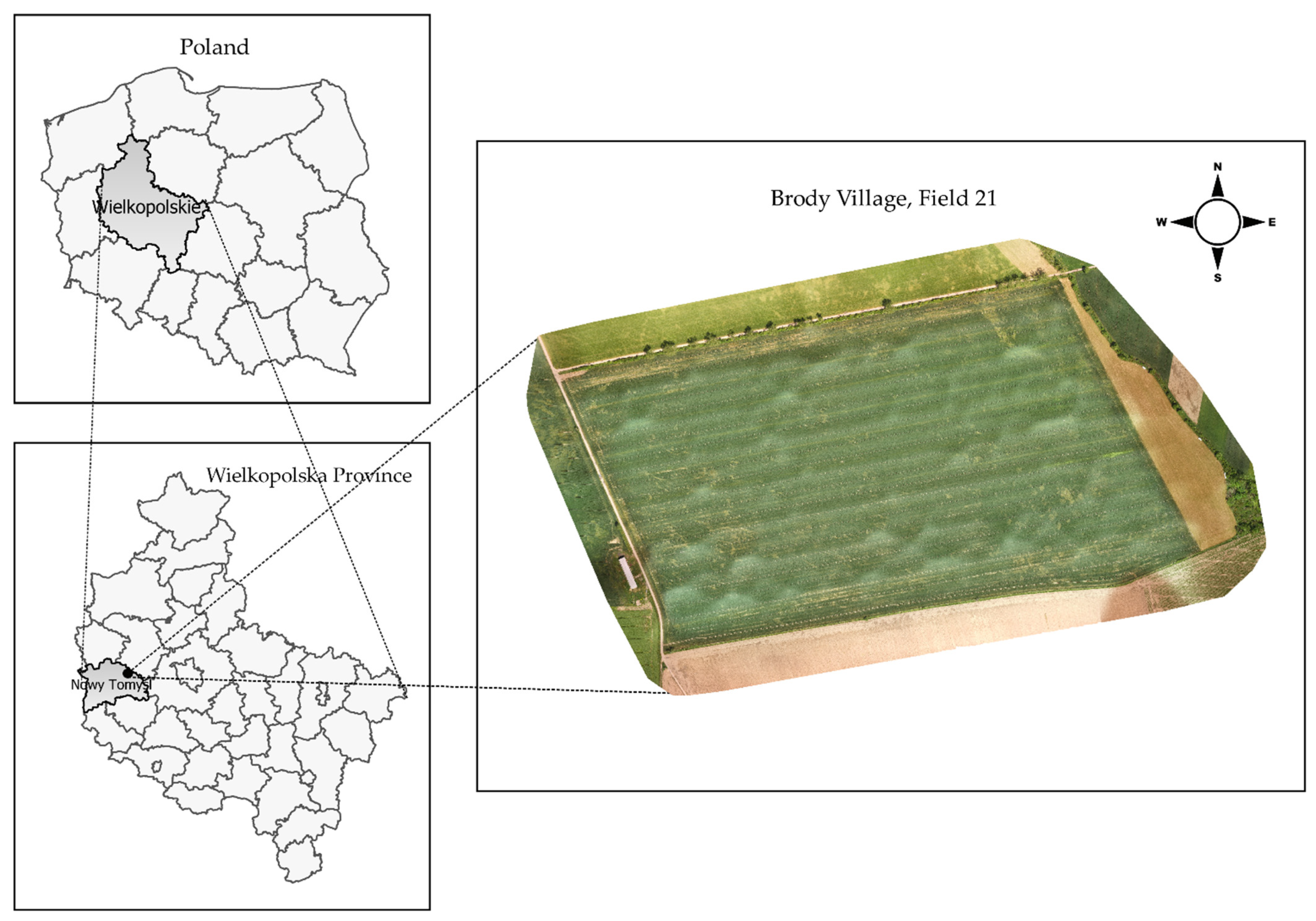
2.1. Study Area
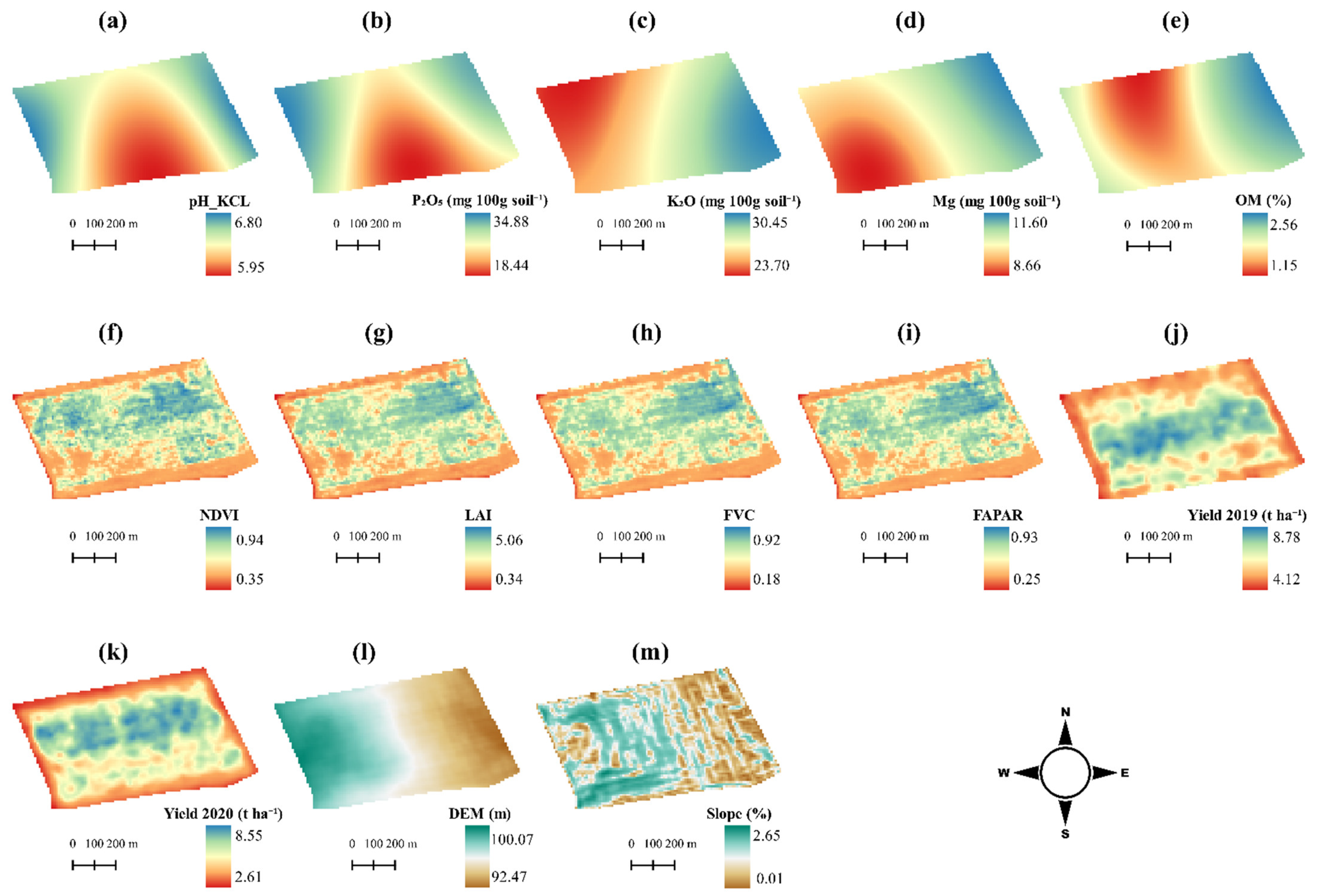
2.2. Data
2.2.1. Soil Sampling
2.2.2. Yield Data
2.2.3. Elevation Data
2.2.4. RS Data
2.3. Models
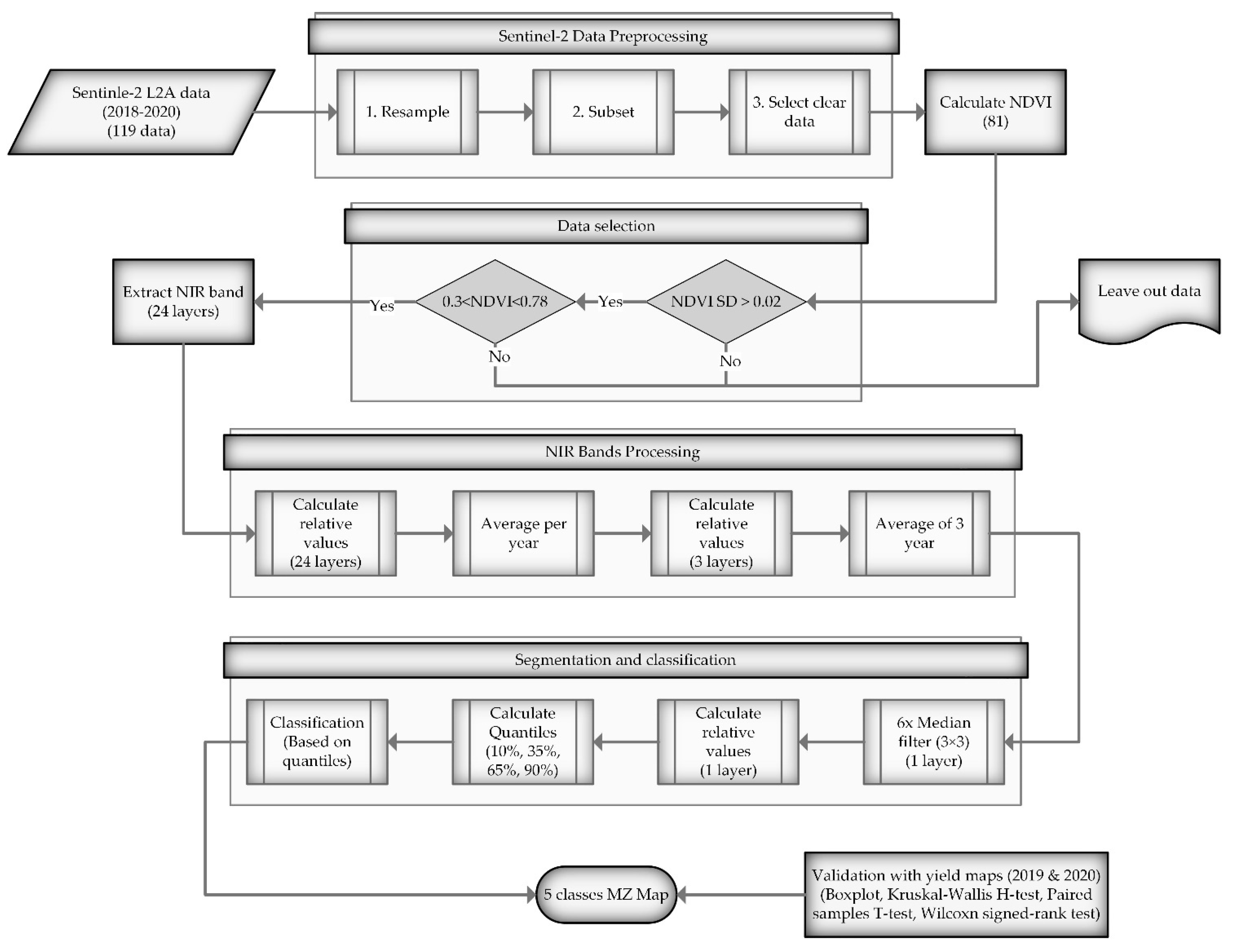
2.3.1. Model-1 (RS- and Threshold-Based Clustering)
Sentinel-2 Data Processing
Data Selection
Processing of NIR Bands
Segmentation and Classification
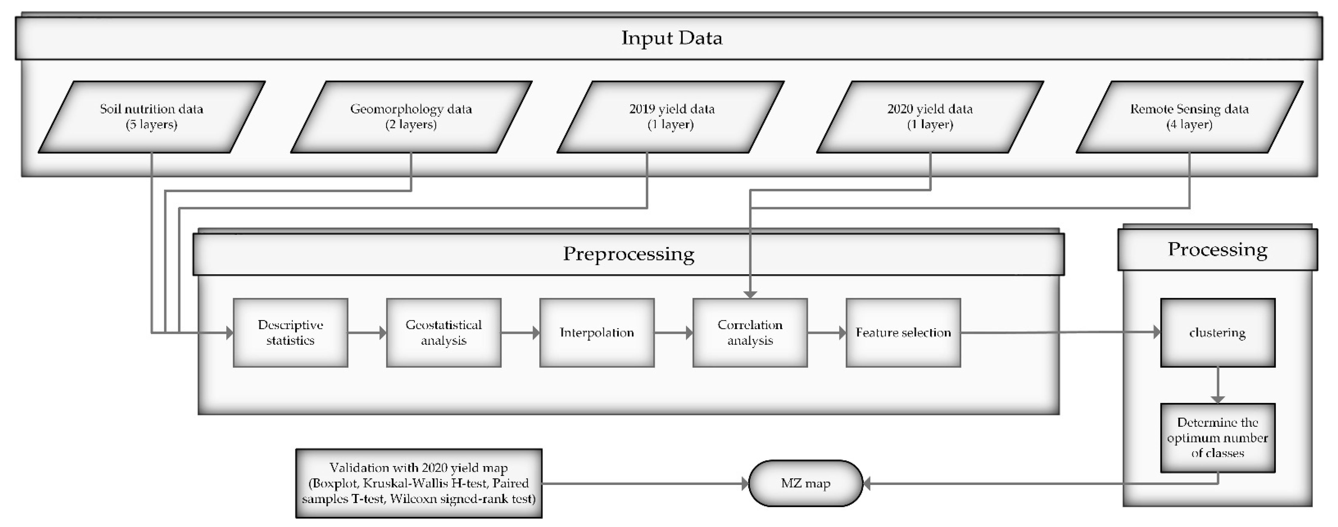
2.3.2. Model-2 (Hybrid-Based, Unsupervised Clustering)
Input Data
Preprocessing
Processing
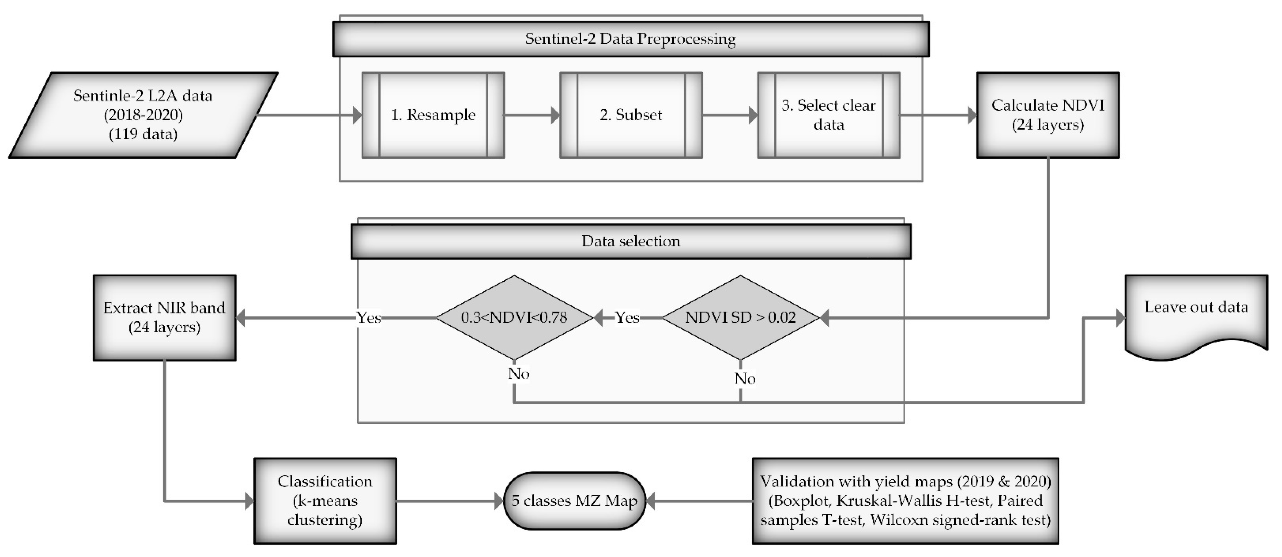
2.3.3. Model-3 (RS-Based, Unsupervised Clustering)
2.4. Model Improvement
2.5. Sampling for Validation
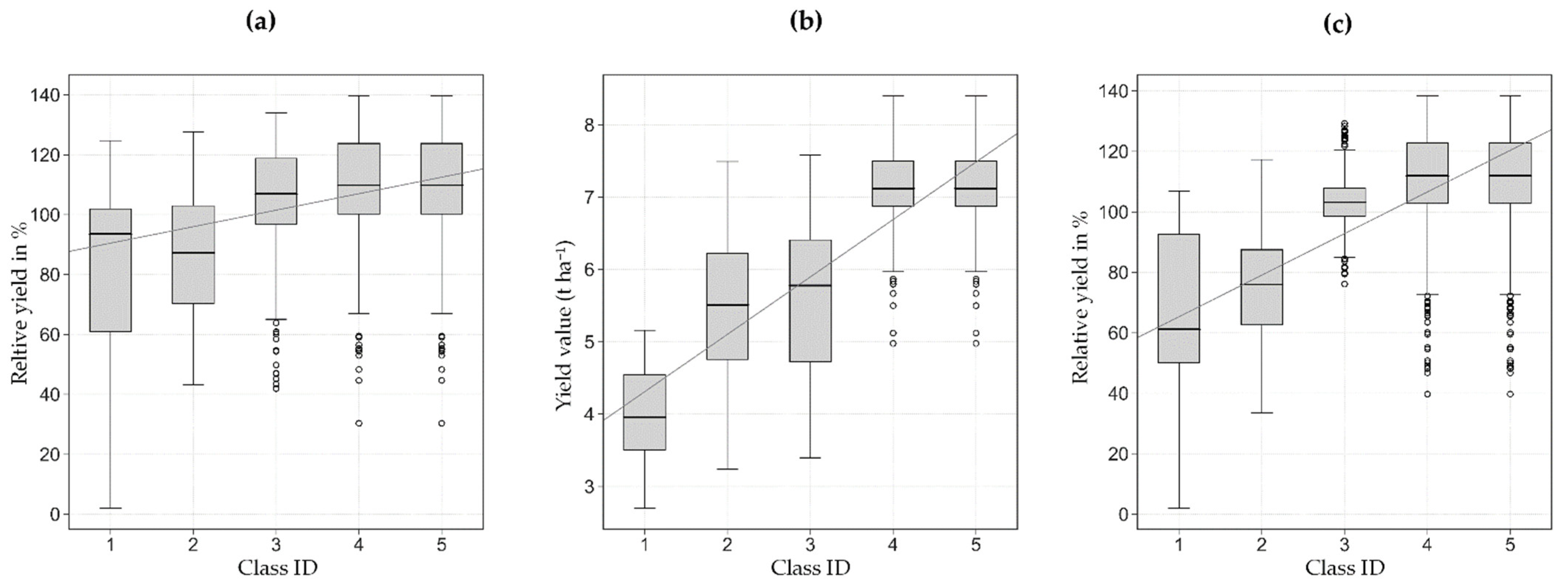
2.6. Validation
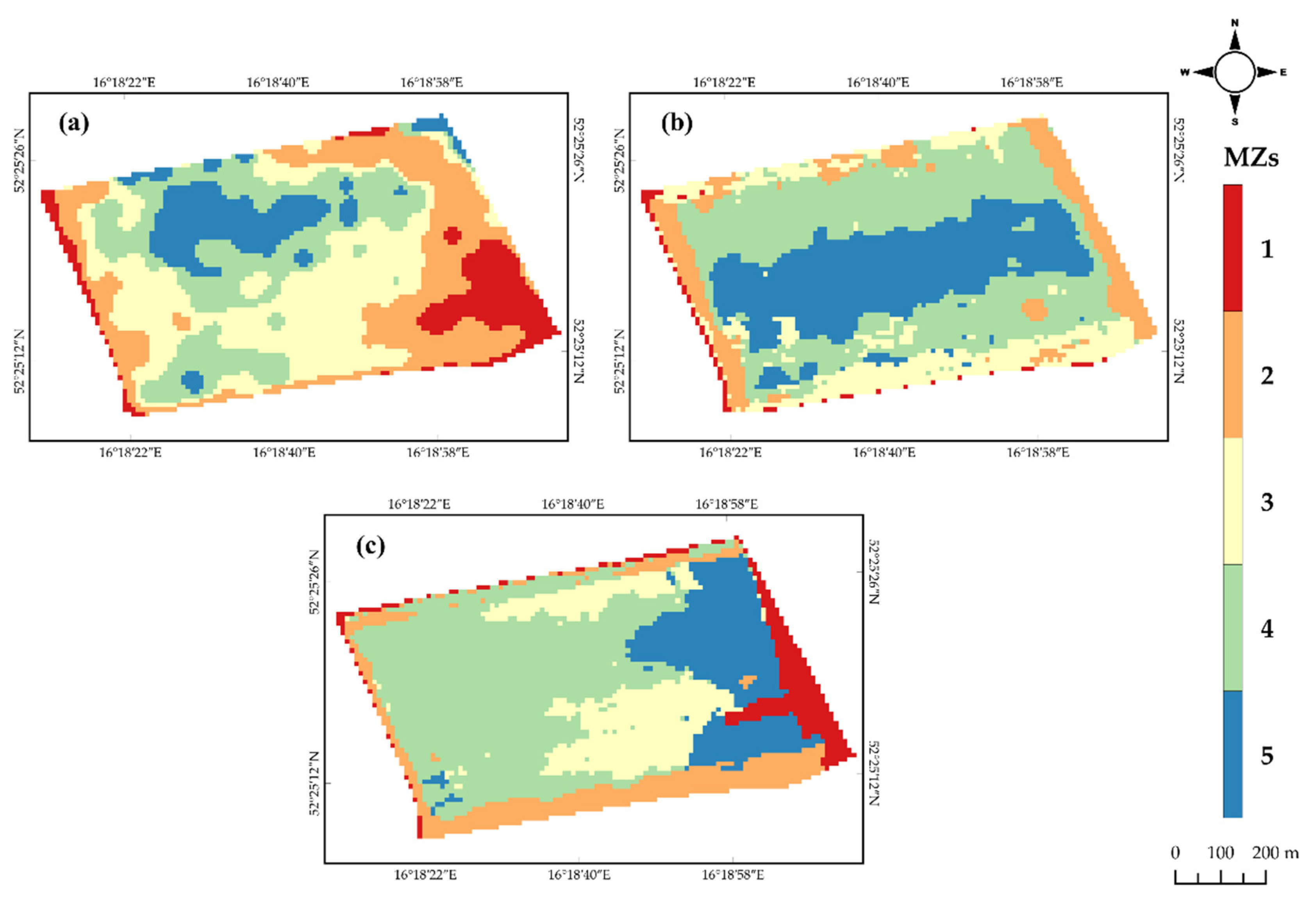
3. Results
3.1. Model-1
3.2. Model-2
3.3. Model-3
3.4. Improvement of Model Results
3.4.1. Model-1
3.4.2. Model-3
4. Discussion
5. Conclusions
Supplementary Materials
Author Contributions
Funding
Institutional Review Board Statement
Informed Consent Statement
Data Availability Statement
Acknowledgments
Conflicts of Interest
References
- Assembly, G. United Nations: Transforming Our World: The 2030 Agenda for Sustainable Development; UN: New York, NY, USA, 2015. [Google Scholar]
- Nawar, S.; Corstanje, R.; Halcro, G.; Mulla, D.; Mouazen, A.M. Delineation of Soil Management Zones for Variable-Rate Fertilization. Adv. Agron. 2017, 143, 175–245. [Google Scholar] [CrossRef]
- Foley, J.A.; Ramankutty, N.; Brauman, K.A.; Cassidy, E.S.; Gerber, J.S.; Johnston, M.; Mueller, N.D.; O’Connell, C.; Ray, D.K.; West, P.C.; et al. Solutions for a cultivated planet. Nature 2011, 478, 337–342. [Google Scholar] [CrossRef] [PubMed] [Green Version]
- Sims, B.; Kienzle, J. Sustainable Agricultural Mechanization for Smallholders: What Is It and How Can We Implement It? Agriculture 2017, 7, 50. [Google Scholar] [CrossRef] [Green Version]
- Larkin, D.L.; Lozada, D.N.; Mason, R.E. Genomic Selection—Considerations for Successful Implementation in Wheat Breeding Programs. Agronomy 2019, 9, 479. [Google Scholar] [CrossRef] [Green Version]
- Gebbers, R.; Adamchuk, V.I. Precision agriculture and food security. Science 2010, 327, 828–831. [Google Scholar] [CrossRef]
- Lee, C.-L.; Strong, R.; Dooley, K.E. Analyzing Precision Agriculture Adoption across the Globe: A Systematic Review of Scholarship from 1999–2020. Sustainability 2021, 13, 10295. [Google Scholar] [CrossRef]
- Lajoie-O’Malley, A.; Bronson, K.; van der Burg, S.; Klerkx, L. The future(s) of digital agriculture and sustainable food systems: An analysis of high-level policy documents. Ecosyst. Serv. 2020, 45, 101183. [Google Scholar] [CrossRef]
- Pierce, F.J.; Nowak, P. Aspects of precision agriculture. Adv. Agron. 1999, 67, 1–85. [Google Scholar]
- Bongiovanni, R.; Lowenberg-DeBoer, J. Precision agriculture and sustainability. Precis. Agric. 2004, 5, 359–387. [Google Scholar] [CrossRef]
- Mueller, N.D.; Gerber, J.S.; Johnston, M.; Ray, D.K.; Ramankutty, N.; Foley, J.A. Closing yield gaps through nutrient and water management. Nature 2012, 490, 254–257. [Google Scholar] [CrossRef]
- Liaghat, S.; Balasundram, S.K. A review: The role of remote sensing in precision agriculture. Am. J. Agric. Biol. Sci. 2010, 5, 50–55. [Google Scholar]
- Wojciechowski, T.; Niedbała, G.; Czechlowski, M.; Nawrocka, J.R.; Piechnik, L.; Niemann, J. Rapeseed seeds quality classification with usage of VIS-NIR fiber optic probe and artificial neural networks. In Proceedings of the 2016 International Conference on Optoelectronics and Image Processing (ICOIP), Warsaw, Poland, 10–12 June 2016; pp. 44–48. [Google Scholar]
- Niazian, M.; Niedbała, G. Machine Learning for Plant Breeding and Biotechnology. Agriculture 2020, 10, 436. [Google Scholar] [CrossRef]
- Szwedziak, K.; Polańczyk, E.; Grzywacz, Ż.; Niedbała, G.; Wojtkiewicz, W. Neural Modeling of the Distribution of Protein, Water and Gluten in Wheat Grains during Storage. Sustainability 2020, 12, 5050. [Google Scholar] [CrossRef]
- Mulla, D.J. Twenty five years of remote sensing in precision agriculture: Key advances and remaining knowledge gaps. Biosyst. Eng. 2013, 114, 358–371. [Google Scholar] [CrossRef]
- Georgi, C.; Spengler, D.; Itzerott, S.; Kleinschmit, B. Automatic delineation algorithm for site-specific management zones based on satellite remote sensing data. Precis. Agric. 2017, 19, 684–707. [Google Scholar] [CrossRef] [Green Version]
- Cisternas, I.; Velásquez, I.; Caro, A.; Rodríguez, A. Systematic literature review of implementations of precision agriculture. Comput. Electron. Agric. 2020, 176, 105626. [Google Scholar]
- Vrindts, E.; Mouazen, A.M.; Reyniers, M.; Maertens, K.; Maleki, M.R.; Ramon, H.; De Baerdemaeker, J. Management Zones based on Correlation between Soil Compaction, Yield and Crop Data. Biosyst. Eng. 2005, 92, 419–428. [Google Scholar] [CrossRef]
- Fleming, K.; Heermann, D.; Westfall, D. Evaluating soil color with farmer input and apparent soil electrical conductivity for management zone delineation. Agron. J. 2004, 96, 1581–1587. [Google Scholar] [CrossRef]
- Van Alphen, B.; Stoorvogel, J. A Methodology to Define Management Units in Support of an Integrated, Model-Based Approach to Precision Agriculture. In Proceedings of the Fourth International Conference on Precision Agriculture, Saint Paul, MN, USA, 19–22 July 1998; pp. 1265–1278. [Google Scholar]
- Nolan, S.; Goddard, T.; Lohstraeter, G.; Coen, G. Assessing managements units on rolling topography. In Proceedings of the 5th International Conference on Precision Agriculture, Bloomington, MN, USA, 16–19 July, 2000; pp. 1–12. [Google Scholar]
- Fraisse, C.; Sudduth, K.; Kitchen, N. Delineation of site-specific management zones by unsupervised classification of topographic attributes and soil electrical conductivity. Trans. ASAE 2001, 44, 155. [Google Scholar] [CrossRef] [Green Version]
- Fu, Q.; Wang, Z.; Jiang, Q. Delineating soil nutrient management zones based on fuzzy clustering optimized by PSO. Math. Comput. Model. 2010, 51, 1299–1305. [Google Scholar] [CrossRef]
- MacMillan, R.; Pettapiece, W.; Watson, L.; Goddard, T. A landform segmentation model for precision farming. In Proceedings of the Fourth International Conference on Precision Agriculture, Saint Paul, MN, USA, 19–22 July 1998; pp. 1335–1346. [Google Scholar]
- Taylor, R.; Kluitenberg, G.; Schrock, M.; Zhang, N.; Schmidt, J.; Havlin, J. Using Yield Monitor Data To Determine Spati Al Crop Production Potential. Trans. ASAE 2001, 44, 1409. [Google Scholar]
- Diker, K.; Heermann, D.; Brodahl, M. Frequency analysis of yield for delineating yield response zones. Precis. Agric. 2004, 5, 435–444. [Google Scholar] [CrossRef]
- Milne, A.E.; Webster, R.; Ginsburg, D.; Kindred, D. Spatial multivariate classification of an arable field into compact management zones based on past crop yields. Comput. Electron. Agric. 2012, 80, 17–30. [Google Scholar] [CrossRef]
- Niedbała, G.; Kozlowski, J. Application of artificial neural networks for multi-criteria yield prediction of winter wheat. J. Agric. Sci. Technol. 2019, 21, 51–61. [Google Scholar]
- Niedbała, G.; Nowakowski, K.; Rudowicz-Nawrocka, J.; Piekutowska, M.; Weres, J.; Tomczak, R.J.; Tyksiński, T.; Álvarez Pinto, A. Multicriteria prediction and simulation of winter wheat yield using extended qualitative and quantitative data based on artificial neural networks. Appl. Sci. 2019, 9, 2773. [Google Scholar] [CrossRef] [Green Version]
- Hara, P.; Piekutowska, M.; Niedbała, G. Selection of Independent Variables for Crop Yield Prediction Using Artificial Neural Network Models with Remote Sensing Data. Land 2021, 10, 609. [Google Scholar] [CrossRef]
- Kitchen, N.R.; Sudduth, K.A.; Myers, D.B.; Drummond, S.T.; Hong, S.Y. Delineating productivity zones on claypan soil fields using apparent soil electrical conductivity. Comput. Electron. Agric. 2005, 46, 285–308. [Google Scholar] [CrossRef]
- Cambouris, A.; Nolin, M.; Zebarth, B.; Laverdière, M. Soil management zones delineated by electrical conductivity to characterize spatial and temporal variations in potato yield and in soil properties. Am. J. Potato Res. 2006, 83, 381–395. [Google Scholar]
- Ahn, C.W.; Baumgardner, M.; Biehl, L. Delineation of soil variability using geostatistics and fuzzy clustering analyses of hyperspectral data. Soil Sci. Soc. Am. J. 1999, 63, 142–150. [Google Scholar]
- Vizzari, M.; Santaga, F.; Benincasa, P. Sentinel 2-Based Nitrogen VRT Fertilization in Wheat: Comparison between Traditional and Simple Precision Practices. Agronomy 2019, 9, 278. [Google Scholar] [CrossRef] [Green Version]
- Fridgen, J.J.; Kitchen, N.R.; Sudduth, K.A.; Drummond, S.T.; Wiebold, W.J.; Fraisse, C.W. Management Zone Analyst (MZA) Software for Subfield Management Zone Delineation. Agron. J. 2004, 96, 100–108. [Google Scholar]
- Song, X.; Wang, J.; Huang, W.; Liu, L.; Yan, G.; Pu, R. The delineation of agricultural management zones with high resolution remotely sensed data. Precis. Agric. 2009, 10, 471–487. [Google Scholar] [CrossRef]
- De Benedetto, D.; Castrignanò, A.; Rinaldi, M.; Ruggieri, S.; Santoro, F.; Figorito, B.; Gualano, S.; Diacono, M.; Tamborrino, R. An approach for delineating homogeneous zones by using multi-sensor data. Geoderma 2013, 199, 117–127. [Google Scholar] [CrossRef]
- Yao, R.-J.; Yang, J.-S.; Zhang, T.-J.; Gao, P.; Wang, X.-P.; Hong, L.-Z.; Wang, M.-W. Determination of site-specific management zones using soil physico-chemical properties and crop yields in coastal reclaimed farmland. Geoderma 2014, 232–234, 381–393. [Google Scholar] [CrossRef]
- Farid, H.U.; Bakhsh, A.; Ahmad, N.; Ahmad, A.; Mahmood-Khan, Z. Delineating site-specific management zones for precision agriculture. J. Agric. Sci. 2015, 154, 273–286. [Google Scholar] [CrossRef]
- Peralta, N.R.; Costa, J.L.; Balzarini, M.; Castro Franco, M.; Córdoba, M.; Bullock, D. Delineation of management zones to improve nitrogen management of wheat. Comput. Electron. Agric. 2015, 110, 103–113. [Google Scholar] [CrossRef]
- Basso, B.; Dumont, B.; Cammarano, D.; Pezzuolo, A.; Marinello, F.; Sartori, L. Environmental and economic benefits of variable rate nitrogen fertilization in a nitrate vulnerable zone. Sci. Total Environ. 2016, 545–546, 227–235. [Google Scholar] [CrossRef] [Green Version]
- Gavioli, A.; de Souza, E.G.; Bazzi, C.L.; Guedes, L.P.C.; Schenatto, K. Optimization of management zone delineation by using spatial principal components. Comput. Electron. Agric. 2016, 127, 302–310. [Google Scholar] [CrossRef]
- Oldoni, H.; Silva Terra, V.S.; Timm, L.C.; Júnior, C.R.; Monteiro, A.B. Delineation of management zones in a peach orchard using multivariate and geostatistical analyses. Soil Tillage Res. 2019, 191, 1–10. [Google Scholar] [CrossRef]
- Gavioli, A.; de Souza, E.G.; Bazzi, C.L.; Schenatto, K.; Betzek, N.M. Identification of management zones in precision agriculture: An evaluation of alternative cluster analysis methods. Biosyst. Eng. 2019, 181, 86–102. [Google Scholar] [CrossRef]
- Moharana, P.C.; Jena, R.K.; Pradhan, U.K.; Nogiya, M.; Tailor, B.L.; Singh, R.S.; Singh, S.K. Geostatistical and fuzzy clustering approach for delineation of site-specific management zones and yield-limiting factors in irrigated hot arid environment of India. Precis. Agric. 2019, 21, 426–448. [Google Scholar] [CrossRef]
- Nogueira Martins, R.; Magalhães Valente, D.S.; Fim Rosas, J.T.; Souza Santos, F.; Lima Dos Santos, F.F.; Nascimento, M.; Campana Nascimento, A.C. Site-specific Nutrient Management Zones in Soybean Field Using Multivariate Analysis: An Approach Based on Variable Rate Fertilization. Commun. Soil Sci. Plant. Anal. 2020, 51, 687–700. [Google Scholar] [CrossRef]
- Gotway, C.; Ferguson, R.; Hergert, G. The Effects of Mapping and Scale on Variable-Rate Fertilizer Recommendations for Corn. In Proceedings of the Third International Conference on Precision Agriculture, Minneapolis, MN, USA, 23–26 June 1996; pp. 321–330. [Google Scholar]
- Fleming, K.; Westfall, D.; Bausch, W. Evaluating management zone technology and grid soil sampling for variable rate nitrogen application. In Proceedings of the 5th International Conference on Precision Agriculture, Bloomington, MN, USA, 16–19 July 2000; pp. 16–19. [Google Scholar]
- Koch, B.; Khosla, R. The Role of Precision Agriculture in Cropping Systems. J. Crop. Prod. 2003, 9, 361–381. [Google Scholar] [CrossRef]
- Cohen, S.; Cohen, Y.; Alchanatis, V.; Levi, O. Combining spectral and spatial information from aerial hyperspectral images for delineating homogenous management zones. Biosyst. Eng. 2013, 114, 435–443. [Google Scholar] [CrossRef]
- Basnyat, P.; McConkey, B.G.; Selles, F.; Meinert, L.B. Effectiveness of using vegetation index to delineate zones of different soil and crop grain production characteristics. Can. J. Soil Sci. 2005, 85, 319–328. [Google Scholar] [CrossRef]
- Oza, S.R.; Panigrahy, S.; Parihar, J.S. Concurrent use of active and passive microwave remote sensing data for monitoring of rice crop. Int. J. Appl. Earth Obs. Geoinf. 2008, 10, 296–304. [Google Scholar] [CrossRef]
- Segarra, J.; Buchaillot, M.L.; Araus, J.L.; Kefauver, S.C. Remote Sensing for Precision Agriculture: Sentinel-2 Improved Features and Applications. Agronomy 2020, 10, 641. [Google Scholar] [CrossRef]
- European Space Agency (ESA). MultiSpectral Instrument (MSI) Overview. Available online: https://sentinels.copernicus.eu/web/sentinel/technical-guides/sentinel-2-msi/msi-instrument (accessed on 20 October 2021).
- European Space Agency (ESA). Sentinel-2 (MSI) Overview. Available online: https://sentinel.esa.int/web/sentinel/missions/sentinel-2 (accessed on 20 October 2021).
- European Space Agency (ESA). Data Products (MSI) Overview. Available online: https://sentinels.copernicus.eu/web/sentinel/missions/sentinel-2/data-products (accessed on 20 October 2021).
- Rouse, J.W.; Haas, R.H.; Schell, J.A.; Deering, D.W. Monitoring vegetation systems in the Great Plains with ERTS. NASA Spec. Publ. 1974, 351, 309. [Google Scholar]
- Weiss, M.; Baret, F. S2ToolBox Level 2 Products: LAI, FAPAR, FCOVER, Version 1.1. Available online: https://step.esa.int/docs/extra/ATBD_S2ToolBox_L2B_V1.1.pdf (accessed on 20 October 2021).
- Song, W.; Mu, X.; Ruan, G.; Gao, Z.; Li, L.; Yan, G. Estimating fractional vegetation cover and the vegetation index of bare soil and highly dense vegetation with a physically based method. Int. J. Appl. Earth Obs. Geoinf. 2017, 58, 168–176. [Google Scholar]
- Kosior, K. Łańcuch wartości dużych zbiorów danych (big data) w rolnictwie–problemy i wyzwania regulacyjne. Studia BAS 2020, 3, 101–125. [Google Scholar] [CrossRef]
- Santaga, F.S.; Benincasa, P.; Toscano, P.; Antognelli, S.; Ranieri, E.; Vizzari, M. Simplified and Advanced Sentinel-2-Based Precision Nitrogen Management of Wheat. Agronomy 2021, 11, 1156. [Google Scholar]
- Majchrzak, L.; Sawinska, Z.; Natywa, M.; Skrzypczak, G.; Głowicka-Wołoszyn, R. Impact of different tillage systems on soil dehydrogenase activity and spring wheat infection. J. Agric. Sci. Technol. 2016, 18, 1871–1881. [Google Scholar]
- Tryjanowski, P.; Sparks, T.H.; Blecharczyk, A.; Małecka-Jankowiak, I.; Switek, S.; Sawinska, Z. Changing Phenology of Potato and of the Treatment for its Major Pest (Colorado Potato Beetle)—A Long-term Analysis. Am. J. Potato Res. 2017, 95, 26–32. [Google Scholar] [CrossRef] [Green Version]
- Egnér, H.; Riehm, H.; Domingo, W. Untersuchungen über die chemische Bodenanalyse als Grundlage für die Beurteilung des Nährstoffzustandes der Böden. II. Chem. Extra Ktionsmethoden Zur Phosphor-Und Kaliumbestimmung K. Lantbr. Ann. 1960, 26, 199–215. [Google Scholar]
- Schachtschabel, P.V. Das pflanzenverfügbare Magnesium des Boden und seine Bestimmung. Z. Für Pflanz. Düngung Bodenkd. 1954, 67, 9–23. [Google Scholar] [CrossRef]
- Tiurin, I. К mietodikie analiza dla srawnitielnogo izuczenia sostawa poczwiennogo gumusa. Tr. Poczw. Inst. AN SSSR 1951, 38, 1–250. [Google Scholar]
- Czechlowski, M.; Wojciechowski, T. The utilization of information about local variable environmental conditions to predict the quality of wheat grain during the harvest. J. Res. Appl. Agric. Eng. 2013, 58, 31–34. [Google Scholar]
- Czechlowski, M.; Wojciechowski, T. System mechatroniczny do selektywnego zbioru ziarna zbóż. Zeszyty Naukowe Instytutu Pojazdów 2013, 4, 95. [Google Scholar]
- Czechlowski, M.; Wojciechowski, T.; Adamski, M.; Niedbała, G.; Piekutowska, M. Application of ASG-EUPOS high precision positioning system for cereal harvester monitoring. J. Res. Appl. Agric. Eng. 2018, 63, 44–50. [Google Scholar]
- European Space Agency (ESA). Copernicus Open Access Hub. Available online: https://scihub.copernicus.eu/ (accessed on 20 October 2021).
- European Space Agency (ESA). STEP-Scientific Toolbox Exploitation Platform Ver 7.0. Available online: https://step.esa.int/main/ (accessed on 20 October 2021).
- Liang, S. Quantitative Remote Sensing of Land Surfaces; John Wiley & Sons Inc.: Hoboken, NJ, USA, 2005; Volume 30. [Google Scholar]
- Lillesand, T.; Kiefer, R.W.; Chipman, J. Remote Sensing and Image Interpretation; John Wiley & Sons Inc.: Hoboken, NJ, USA, 2015. [Google Scholar]
- QGIS, Version 3.10.8. Available online: https://www.qgis.org/en/site/ (accessed on 8 February 2021).
- Webster, R.; Oliver, M.A. Geostatistics for Environmental Scientists; John Wiley & Sons Inc.: Hoboken, NJ, USA, 2007. [Google Scholar]
- ArcGIS, Version 10.7. Available online: https://desktop.arcgis.com/en/arcmap/ (accessed on 8 February 2021).
- Management Zone Analyst (MZA), Version 1.0. Available online: https://www.ars.usda.gov/research/software/download/?softwareid=24&modecode=50-70-10-00 (accessed on 8 February 2021).
- Odeh, I.; McBratney, A.; Chittleborough, D. Soil pattern recognition with fuzzy-c-means: Application to classification and soil-landform interrelationships. Soil Sci. Soc. Am. J. 1992, 56, 505–516. [Google Scholar] [CrossRef]
- Boydell, B.; McBratney, A. Identifying potential within-field management zones from cotton-yield estimates. Precis. Agric. 2002, 3, 9–23. [Google Scholar]
- Bezdek, J.C. Pattern Recognition with Fuzzy Objective Function Algorithms; Springer: Boston, MA, USA, 1981; pp. 43–93. [Google Scholar]
- Olofsson, P.; Foody, G.M.; Herold, M.; Stehman, S.V.; Woodcock, C.E.; Wulder, M.A. Good practices for estimating area and assessing accuracy of land change. Remote. Sens. Environ. 2014, 148, 42–57. [Google Scholar] [CrossRef]
- Pińskwar, I.; Choryński, A.; Kundzewicz, Z.W. Severe Drought in the Spring of 2020 in Poland—More of the Same? Agronomy 2020, 10, 1646. [Google Scholar] [CrossRef]
- Warrick, A. Spatial variability of soil physical properties in the field. Appl. Soil Phys. 1980, 319–344. [Google Scholar] [CrossRef]
- Cambardella, C.A.; Moorman, T.B.; Novak, J.; Parkin, T.; Karlen, D.; Turco, R.; Konopka, A. Field-scale variability of soil properties in central Iowa soils. Soil Sci. Soc. Am. J. 1994, 58, 1501–1511. [Google Scholar] [CrossRef]
- Reza, S.K.; Nayak, D.C.; Mukhopadhyay, S.; Chattopadhyay, T.; Singh, S.K. Characterizing spatial variability of soil properties in alluvial soils of India using geostatistics and geographical information system. Arch. Agron. Soil Sci. 2017, 63, 1489–1498. [Google Scholar] [CrossRef]
- Giua, C.; Materia, V.C.; Camanzi, L. Management information system adoption at the farm level: Evidence from the literature. Br. Food J. 2020, 123, 884–909. [Google Scholar] [CrossRef]


| Month | Jan | Feb | Mar | Apr | May | June | July | Aug | Sep | Oct | Nov | Dec | |
|---|---|---|---|---|---|---|---|---|---|---|---|---|---|
| Year | |||||||||||||
| 2018 | 1 | 2 | 1 | 5 | 8 | 2 | 6 | 7 | 5 | 8 | 2 | 1 | |
| 2019 | 0 | 4 | 2 | 6 | 5 | 8 | 3 | 3 | 5 | 5 | 2 | 4 | |
| 2020 | 3 | 3 | 4 | 7 | 4 | 3 | - * | - * | - * | - * | - * | - * | |
| Data | Data | Data |
|---|---|---|
| 25 February 2018 | 8 February 2019 | 20 February 2020 |
| 6 April 2018 | 18 February 2019 | 11 March 2020 |
| 9 April 2018 | 25 February 2019 | 5 April 2020 |
| 31 May 2018 | 28 February 2019 | 8 April 2020 |
| 3 June 2018 | 18 June 2019 | 22 June 2020 |
| 8 June 2018 | 20 June 2019 | |
| 3 July 2018 | 25 June 2019 | |
| 31 October 2018 | 24 August 2019 | |
| 7 November 2018 | 27 August 2019 | |
| 5 December 2018 | ||
| Total in 2018: 10 | Total in 2019: 9 | Total in 2020: 5 |
| Attributes | n | Min | Max | Mean | SD | SE | CV | Skewness | Kurtosis |
|---|---|---|---|---|---|---|---|---|---|
| DEM 2020 (m) | 67,158 | 92.42 | 100.12 | 96.21 | 2.36 | 0.01 | 0.02 | 0.06 | −1.45 |
| OM 2011 (%) | 52 | 1.14 | 2.64 | 1.66 | 0.44 | 0.06 | 0.26 | 0.92 | −0.33 |
| pHKCl 2020 | 14 | 6.00 | 7.1 | 6.44 | 0.32 | 0.08 | 0.05 | 0.44 | −0.45 |
| P2O 2020 (mg 100 g soil−1) | 14 | 17.20 | 36.6 | 25.71 | 5.92 | 1.58 | 0.22 | 0.20 | −1.07 |
| K2O 2020 (mg 100 g soil−1) | 14 | 23.00 | 34.0 | 26.86 | 3.55 | 0.95 | 0.13 | 0.64 | −0.80 |
| Mg 2020 (mg 100 g soil−1) | 14 | 8.50 | 12.4 | 9.89 | 1.41 | 0.38 | 0.14 | 0.70 | −1.04 |
| Yield 2019 (t ha−1) | 9613 | 0.39 | 15.18 | 7.19 | 1.56 | 0.02 | 0.22 | −1.25 | 5.01 |
| Yield 2020 (t ha−1) | 8520 | 0.36 | 13.12 | 6.82 | 1.58 | 0.02 | 0.23 | −1.30 | 3.11 |
| Variables | Model | Nugget (C0) | Partial Sill (C1) | Sill (C0 + C1) | Nugget/Sill C0/(C0 + C1) | Range (m) | RMSE |
|---|---|---|---|---|---|---|---|
| DEM | Exponential | 0 | 0.0005 | 0.0005 | 0 | 1.4042 | 0.0209 |
| OM | J-Bessel | 0.0266 | 0.2443 | 0.2709 | 0.0982 | 1247.5 | 0.1665 |
| pHKCl | J-Bessel | 0.0299 | 0.0778 | 0.1077 | 0.2776 | 925.03 | 0.2391 |
| P2O5 | Hole Effect | 12.883 | 28.331 | 41.214 | 0.3126 | 915.83 | 4.2782 |
| K2O | Gaussian | 6.4560 | 16.516 | 22.972 | 0.2810 | 1147.2 | 2.8914 |
| Mg | Gaussian | 1.0110 | 2.7338 | 3.7448 | 0.2970 | 1147.2 | 1.0427 |
| Yield 2019 | Exponential | 1.6169 | 0.7382 | 2.3551 | 0.6865 | 490.05 | 1.3108 |
| Yield 2020 | Exponential | 1.2226 | 2.2208 | 3.4434 | 0.3550 | 1301.7 | 1.0925 |
Publisher’s Note: MDPI stays neutral with regard to jurisdictional claims in published maps and institutional affiliations. |
© 2021 by the authors. Licensee MDPI, Basel, Switzerland. This article is an open access article distributed under the terms and conditions of the Creative Commons Attribution (CC BY) license (https://creativecommons.org/licenses/by/4.0/).
Share and Cite
Rokhafrouz, M.; Latifi, H.; Abkar, A.A.; Wojciechowski, T.; Czechlowski, M.; Naieni, A.S.; Maghsoudi, Y.; Niedbała, G. Simplified and Hybrid Remote Sensing-Based Delineation of Management Zones for Nitrogen Variable Rate Application in Wheat. Agriculture 2021, 11, 1104. https://0-doi-org.brum.beds.ac.uk/10.3390/agriculture11111104
Rokhafrouz M, Latifi H, Abkar AA, Wojciechowski T, Czechlowski M, Naieni AS, Maghsoudi Y, Niedbała G. Simplified and Hybrid Remote Sensing-Based Delineation of Management Zones for Nitrogen Variable Rate Application in Wheat. Agriculture. 2021; 11(11):1104. https://0-doi-org.brum.beds.ac.uk/10.3390/agriculture11111104
Chicago/Turabian StyleRokhafrouz, Mohammad, Hooman Latifi, Ali A. Abkar, Tomasz Wojciechowski, Mirosław Czechlowski, Ali Sadeghi Naieni, Yasser Maghsoudi, and Gniewko Niedbała. 2021. "Simplified and Hybrid Remote Sensing-Based Delineation of Management Zones for Nitrogen Variable Rate Application in Wheat" Agriculture 11, no. 11: 1104. https://0-doi-org.brum.beds.ac.uk/10.3390/agriculture11111104