Reliable Identification of Oolong Tea Species: Nondestructive Testing Classification Based on Fluorescence Hyperspectral Technology and Machine Learning

Abstract

A rapid and nondestructive tea classification method is of great significance in today’s research. This study uses fluorescence hyperspectral technology and machine learning to distinguish Oolong tea by analyzing the spectral features of tea in the wavelength ranging from 475 to 1100 nm. The spectral data are preprocessed by multivariate scattering correction (MSC) and standard normal variable (SNV), which can effectively reduce the impact of baseline drift and tilt. Then principal component analysis (PCA) and t-distribution random neighborhood embedding (t-SNE) are adopted for feature dimensionality reduction and visual display. Random Forest-Recursive Feature Elimination (RF-RFE) is used for feature selection. Decision Tree (DT), Random Forest Classification (RFC), K-Nearest Neighbor (KNN) and Support Vector Machine (SVM) are used to establish the classification model. The results show that MSC-RF-RFE-SVM is the best model for the classification of Oolong tea in which the accuracy of the training set and test set is 100% and 98.73%, respectively. It can be concluded that fluorescence hyperspectral technology and machine learning are feasible to classify Oolong tea.

1. Introduction

Chinese tea culture has a long history, dating back to the Shennong period [1]. Tea is one of the most popular non-alcoholic drinks [2]. Tea contains many healthy components, such as tea polyphenols, tea polysaccharides, theanine, vitamins and minerals [3], which have refreshing effects, helping digestion, anti-oxidation, anti-cancer and weight loss, which make tea popular with consumers around the world [4]. It is reported that there are over 1 billion tea lovers worldwide which increases the demand in the tea market. As a large tea producing country, China’s export position is very good, with export volumes increasing from 325,800 tonnes in 2013 to 366,600 tonnes in 2019. Affected by the pandemic, China’s exports fell slightly to 348,000 tonnes in 2020, with tea remaining important in the hearts of consumers [5].

Tea is rich in variety and quantity. Due to different processing technologies, growing patterns and other factors, tea quality varies widely, resulting in a price imbalance [6]. In real life, the economic value of quality tea can be several or even tens of times more than that of regular tea [3]. As a result, high pricing of regular tea that looks like quality tea has become one of the common means for illegal businesses to make huge profits [7]. It is difficult for consumers to distinguish the types of tea only with the naked eye, and they often buy cheap tea at a high price, which enables the occurrence of fraud from time to time. To address this situation, this study will use fluorescence hyperspectral technology and machine learning to distinguish Oolong tea [8].

Distinguishing different types of tea or studying tea adulteration can summarize the problem of whether the authenticity of tea can be properly identified [2]. There are many methods of tea classification in current research, which mainly rely on the experience of professionals [8] who, through sensory evaluation, appreciate the color, smell, shape and flavor of tea [9]. This method is not only tedious and time-consuming, but also destroys the structure of tea and causes waste [7]. Conventional analytical techniques have also been used for the classification of tea, such as gas chromatography coupled mass spectrometry (GC–MS) [8,9] and high-performance liquid chromatography (HPLC). The aforementioned chemical methods are costly and time-consuming too, which hinders their prevalence.

With the renewal of detection technology and its innovative application in modern agriculture, scholars use electronic nose, electronic tongue, near infrared spectroscopy (NIRS), and hyperspectral imaging technology (HSI) to classify tea varieties [10]. Dong et al. [11] classified green tea by using a MOS-based electronic nose, with the highest accuracy being 96%.

NIRS [12], a molecular spectra, can comprehensively characterize structural information of the energy level from molecular vibration and reflect the frequency doubling and frequency absorption of hydrogen groups in organic compounds from the vibration of electric dipole moment [13]. Currently, NIRS has been extensively applied for monitoring and classifying tea [14]. Li et al. [15] measured the spectral data of five types of tea by NIRS, carried out cluster analysis on different types of tea by PCA, obtained the principal components of spectral data, and then established a model combined with SVM for variety identification. The prediction accuracy reached 94.29%. Cardoso [16] et al. classified four types of green tea by NIRS, with a classification accuracy of 93%.

HSI [17] is a new conventional spectroscopy and computer-based vision technology [18]. HSI can provide spatial and spectral information on an object by integrating conventional spectroscopic and imaging technology [15]. Hong et al. [19] have studied quality identification and the detection of tea adulteration by using HSI to explore tea classification. Sun et al. [20] identified five types of tea through HSI, optimized the automatic encoder through low-rank matrix recovery, and reduced the dimensions and denoised the spectral data, so as to improve the accuracy of the SVM classification model.

In recent years, the concept of fluorescence spectroscopy has been widely recognized around the world and has grown rapidly [21]. A variety of fluorescence spectra analysis technologies are applied in the detection field, including atomic fluorescence spectrum [22], two-dimensional correlation fluorescence spectra [23], three-dimensional fluorescence spectra [24,25], front surface fluorescence spectra [24], (total) synchronous fluorescence spectra [26] and fluorescence hyperspectral imaging technology [27]. This study is based on fluorescence hyperspectral imaging technology. This technology can simulate human visual function using a computer without damaging to the test samples. This technology can extract color, texture, fluorescence intensity and other information from the fluorescence image for treatment and analysis for practical detection. Because the fluorescence lifetime reflects the attenuation time of fluorescence photons, it is only related to the intensity of excitation light and is not affected by ambient light, fluorescence scattering and other factors, and has the advantages of high sensitivity, high selectivity, convenience, good reproducibility, good stability [28]. Sui et al. [21] analyzed the moisture content of leaves using laser-excitation chlorophyll. Lim et al. [29] used X-ray fluorescence spectra to determine various types of commercial tea. Currently, fluorescence hyperspectral technology and machine learning have not been used to explore tea classification. In this study, a hyperspectral camera is used to obtain a fluorescence image containing the characteristics of a hyperspectral image, which can provide spatial and spectral information, and fluorescence spectral data which contains more detailed information [2]. This is different from the traditional spectroscopy method.

There is a large variety of teas on the market that resemble each other, but a huge difference lies in both quality and price. A new rapid and nondestructive test method will be used for tea classification. In this study, Oolong tea from Anxi County (Huangjingui, Benshan, Maoxie, Jinguanyin, and Tieguanyin) will be cited as an example. Fluorescence hyperspectral spectroscopy and machine learning will be used to detect and classify different types of Oolong tea.

2. Materials and Methods

2.1. Sample

Tea samples used in the study came from Anxi County, Quanzhou, Fujian Province, China. The choice of tea types was made based on the two aspects of appearance and economic value. For the former of these aspects, the selected tea is particle tight and there is little difference in appearance. In terms of economic value, the Tie and Jin varieties have the highest value whereas the price of the remainder of the teas is relatively low. Tie, the best Oolong tea, contains a lot of amino acids, vitamins, minerals, tea polyphenols and alkaloids, and has a variety of nutritional and pharmacodynamic ingredients. Jin takes Tie as a feminine parent and Huang as a masculine parent. Due to the status of its female parent in Oolong tea, its economic value does not differ from Tie. Huang has a slight yellow colour. Ben and Tie are “immediate relatives”, called “the brothers of Tie”. Some Mao has hairy leaves. Ben and Mao are less expensive because they grow and adapt better than Tie. All have the features common to Oolong tea.

Tea samples were supplied by merchants. To ensure the accuracy of the samples, we invited tea experts from Ya’an to identify the types of tea. The verified tea was sent to the laboratory for the acquisition of fluorescence hyperspectral data.

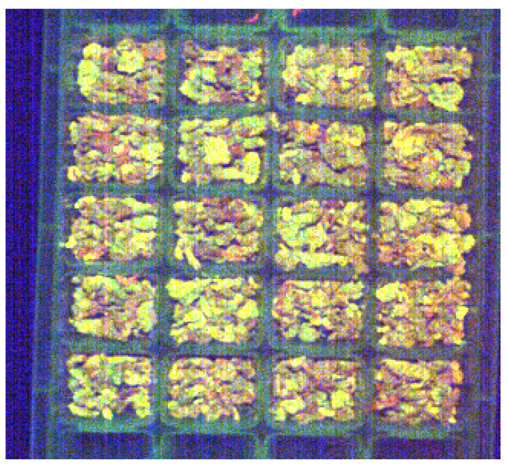
2.2. Fluorescence Hyperspectral Image Acquisition

The fluorescence hyperspectral data of Oolong tea samples were acquired using a GaiaFluo(/Pro)-VN-HR series of fluorescence hyperspectral test system manufactured by Sichuan Dualix Spectral Image Technology Co. Ltd. The hyperspectral camera has the advantages of high sensitivity and high signal-to-noise ratio in the 350 nm to 1100 nm band [30]. The spectral resolution is 2.8 nm with a pixel of 2048 × 946. In the system, the xenon lamp light source was used as the excitation light source for the fluorescence imaging system with a detectable spectral range from 250 nm to 1100 nm [19]. Through the combination of multiple excitation and fluorescence filters, it was found that under the irradiation of four different wave bands of excitation light sources in the laboratory, the 390 nm excitation filter can better cut off the light input of other wave bands. Under the influence of the excitation light source, it is necessary to watch out for the fluorescence signal of the sample. The 475 nm fluorescence filter could complete the separation of the fluorescence signal and parasitic light, so that the final sample captured by the hyperspectral camera produces the best fluorescence signal.

The experiment was performed at an ambient temperature of 26 °C and an ambient humidity of 50%. The RGB channels of the collected fluorescent images were 638, 551 and 442, respectively, the moving speed of the system was 0.26 mm/s, and the camera exposure time was 800 ms. The fluorescence hyperspectral acquisition system is shown in Figure 1. Impacted by the fluorescent filter, the final collected spectral range is 475 nm to 1100 nm, with a total of 104 spectra channels. Samples were placed in the experimental container. A big container can contain 20 small cells, each weighing 2 g. To reduce background interference, the tea sample was evenly and tightly distributed throughout each small cell. 80 samples were taken from each of the five types and a total of 400 samples were collected.

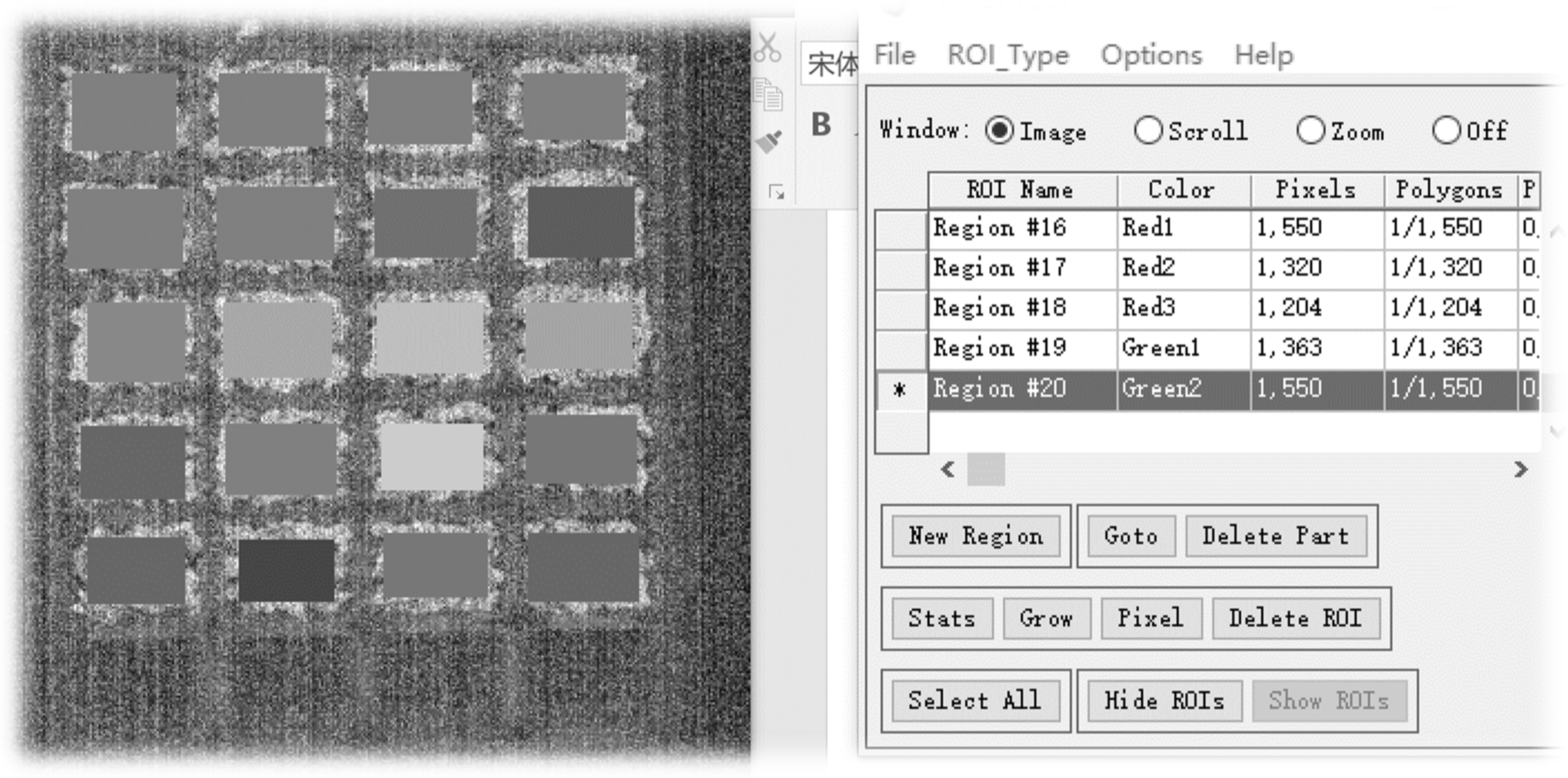
2.3. Fluorescence Hyperspectral Data Extraction

After data collection, it is necessary to extract the spectral data from the image [31]. The region of interest (ROI) [32] is reasonably selected, which is directly related to the quality of the extracted data. In this experiment, ROI were selected through ENVI 5.3 [30]. Using ENVI to set a rectangular box surrounded by 20 samples of each image as ROI and calculating the average value of the spectra of all pixels in the region as the final spectral value of a sample, the extracted data can cover the entire tea sample, avoid the edge of the sample plate and effectively reflect the sample information. The ROI of selected tea samples is shown in Figure 2 and Figure 3. The raw spectral values of tea samples are shown in Figure 4.

Within the spectral range from 475 to 1100 nm, spectral trends are similar. It can be seen from the figure that, due to differences in the quality and internal structure of tea, different types of tea show different fluorescence intensity. The fluorescence intensity of 500–650 nm is not high, which may be explained by the high uptake of chlorophyll and carotenoids [33]. In addition, there are two clear peaks, about 690 nm and 735 nm, respectively [34]. Different types of tea have different peak orientations close to the 690 nm wavelength [17].

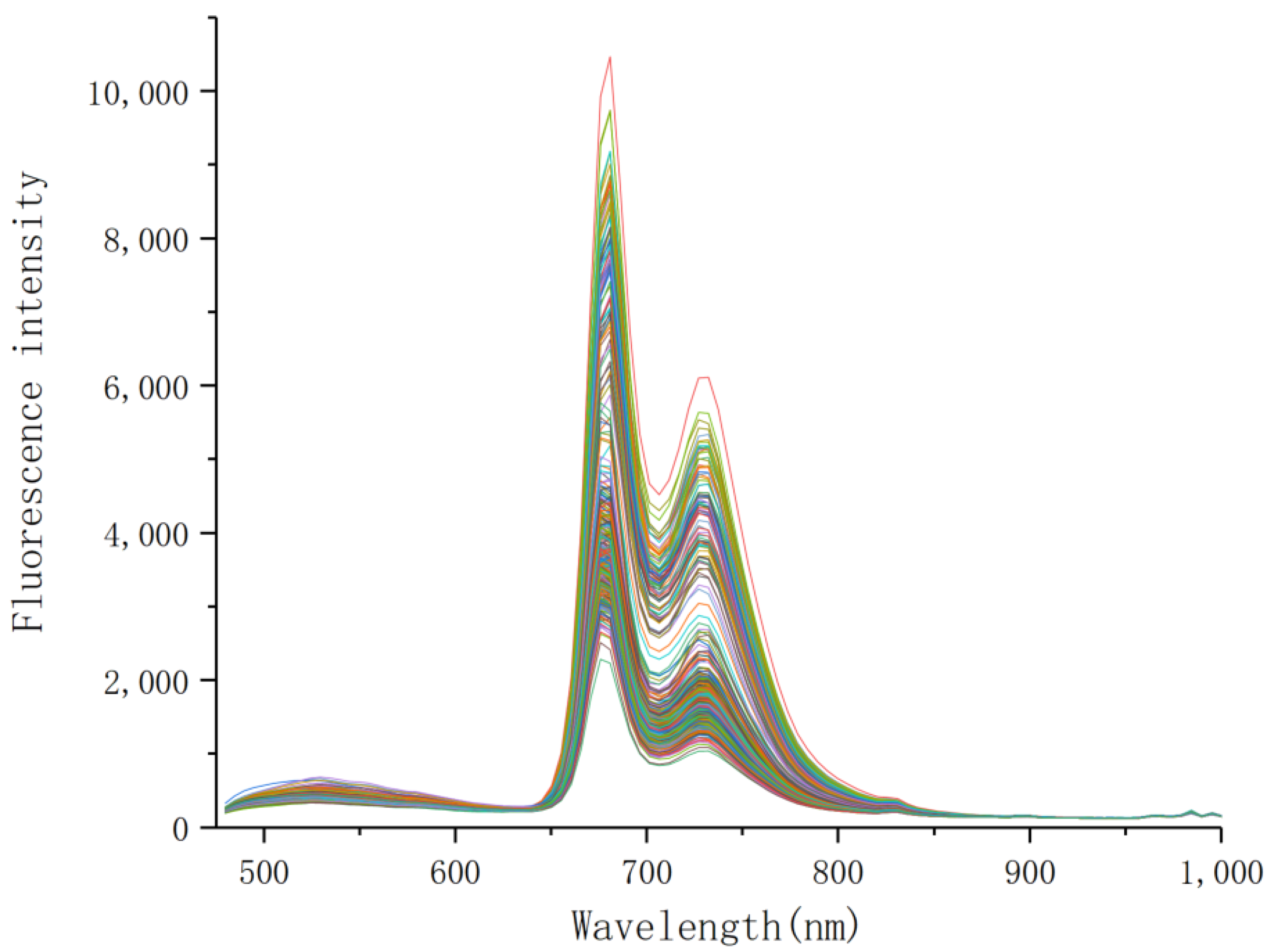
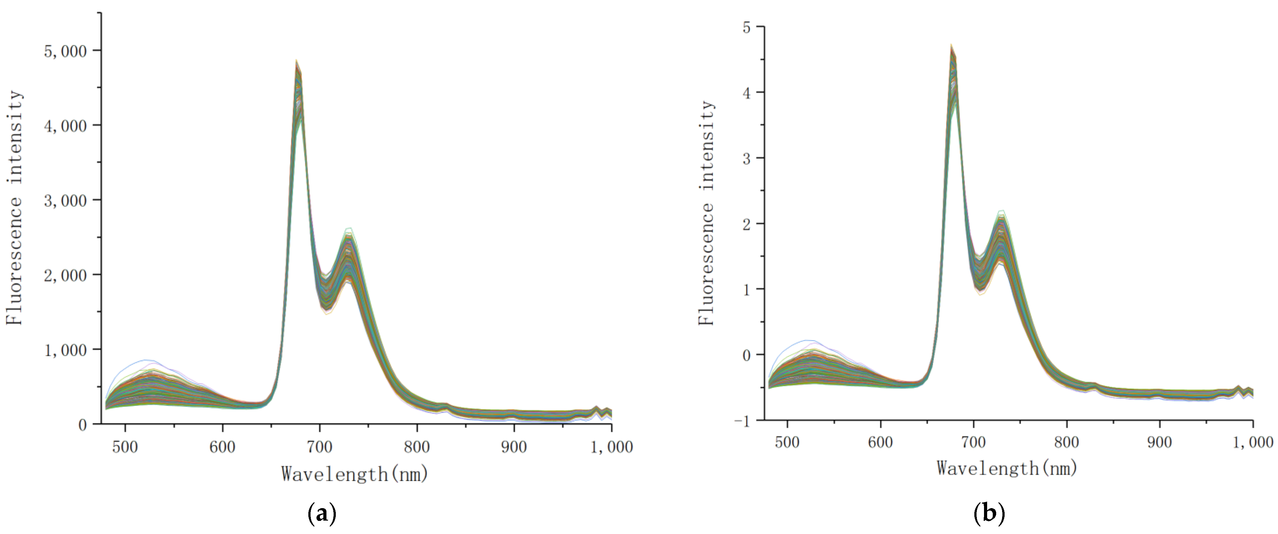
2.4. Spectral Preprocessing

When collecting hyperspectral images of the sample, the effects of the environment, the instrument, the human operation and the sample itself all easily cause a large amount of noise and interference information in the spectral curve [14]. Although the extraction of ROI in the previous work can improve the signal-to-noise ratio of the spectral data, the spectral noise is still unavoidable and has an impact on later qualitative and quantitative modeling analysis [20]. Hence, it is important to exclude spectral noise from the spectral curve as much as possible and to maximize the usefulness of the spectra [35]. In this study multivariate scattering correction (MSC), standard normal variable (SNV), first derivative (FD), second derivative (SD), and wavelet transform (WT) are used for preprocessing. MSC and SNV can effectively reduce the impact of baseline drift, tilt, and other noise [36]. SD and FD processing can effectively reduce the influence of sample background and baseline drift, enhancing the resolution and sensitivity of overlapping peaks [30]. WT has the unique benefits of fine-scaled expression of time, frequency division, multiscale and multiresolution analysis. Four different classification models will be used to assess the effect of preprocessing and verify whether there is an association between the model and the preprocessing method.

2.5. Feature Selection

Spectral data contains a lot of redundant values, collisions, and overlaps. The use of all data to construct a model is complex and time-consuming, while noise and unnecessary information also influence the accuracy and robustness of the model [37]. Currently, the methods of feature processing in machine learning are mainly divided into two types: feature dimensionality reduction and feature selection (include filtering, embedding, and wrapping method) [13]. In this paper, feature dimensionality reduction [20] and feature selection were performed respectively using Principal Component Analysis (PCA) [38], t-distributed stochastic neighbor embedding (t-SNE) [39,40], and random forest-recursive feature elimination (RF-RFE).

2.5.1. Feature Dimensionality Reduction and Data Visualization

PCA is a traditional data dimensional reduction method that has been described in detail in many studies [14]. The main idea of PCA is to map n dimensional features to k dimensional feature, which is a novel orthogonal feature and known as the main component. The k dimensional feature is rebuilt from the original n dimensional features. The work of PCA is to find a set of mutually orthogonal coordinate axes from the original space. The selection of new coordinate axes is closely linked to the data itself [5]. Among the coordinate axes, the first is the direction with the largest variance in the original data, the second is the one with the largest variance in the plane orthogonal to the first, and the third is the one with the largest variance in the plane orthogonal to the first and second. By analogy, many of these can be obtained. Through the new coordinate axes obtained in this way, it is found that most of the variance is contained in the first k coordinate axis, and the variance of the latter two is almost 0, so we can ignore the rest and only keep the first k coordinate axis containing most of the variance.

PCA can reduce the number of features and retain most of the efficient information, which can be used for exploration and visualization of high dimensional data sets, and it has the ability to compress existing features. For dimensional reduction, it uses the data measurement index called sample variance or interpretable variance. The larger the variance, the more information the features have. The variance of the sample is calculated as follows:

$$Var=\frac{1}{n-1}{\displaystyle \sum }_{i=1}^n{\left(x_i-\widehat{x}\right)}^2$$

(1)

where Var is the variance of a feature, n is the number of samples, $x_i$ is the value of each sample in a feature, and $\widehat{x}$ is the mean value of the column of samples.

t-SNE [40] is a manifold learning algorithm based on a random nearest neighbor embedding algorithm (SNE), which is widely used in the field of machine learning and data visualization. It is suitable for the visual display of data points when high dimensional data are reduced to two or three dimensions and can intuitively express the diversity of data. At the same time, t-SNE is also a nonlinear dimensionality reduction algorithm to explore high-dimensional data. The principles of the t-SNE algorithm are as follows [41].

(1)

Joint probability distribution function for measuring the similarity of high dimensional spatial data points.

Let X contain n data points $\left\{x_1,x_2,\dots ,x_n\right\}$, if there are any two data points $x_i$ and $x_j$, $x_j$, which is centered on $x_i$ and whose variance is ${\sigma }_i$, obeys the Gaussian distribution $P_i$. Meanwhile, $x_i$, which is centered on $x_j$ and whose variance is ${\sigma }_j$, obeys the Gaussian distribution $P_j$. The conditional probability of similarity is:

$$p_{j|i}=\frac{\exp \left(-\Vert x_i-x_j\Vert {}^2/2{\sigma }_i^2\right)}{{\sum }_{k\ne i}\exp \left(-\Vert x_i-x_k\Vert {}^2/2{\sigma }_i^2\right)}$$

(2)

where ${\sigma }_j$ can be determined by binary search according to the specified confusion degree $Perp$.

For points in high dimensional space, in order to avoid the influence of outliers, the data points $x_i$ and $x_j$ the joint probability of pairwise similarity in all data points $p_{ij}$ is defined as follows:

$$p_{ij}=\frac{p_{j|i}+p_{i|j}}{2n}$$

(3)

(2)

Joint probability distribution function for measuring the similarity of low dimensional spatial data points.

Let $Y=\left\{y_1,y_2,\dots ,y_n\right\}$ be the low dimensional embedding coordinates of the high dimensional data set $X=\left\{x_1,x_2,\dots ,x_n\right\}$. Assuming that in the low dimensional space, the data points obey the t distribution with a degree of freedom of 1, and then the joint probability $q_{ij}$ of the corresponding points $y_i$ and $y_j$ of the data points $x_i$ and $x_j$ in the low dimensional space is defined as follows:

$$q_{ij}=\frac{{\left(1+\Vert y_i-y_j\Vert {}^2\right)}^{-1}}{{{\displaystyle \sum }}_{k\ne l}{\left(1+\Vert y_k-y_l\Vert {}^2\right)}^{-1}}$$

(4)

(3)

Computational low dimensional embedding

KL divergence is used to measure the similarity between low dimensional spatial probability distribution Q and high dimensional spatial probability distribution P, to obtain the best parameters:

$$C=KL(P\Vert Q)={{\displaystyle \sum }}_i{{\displaystyle \sum }}_j{q}_{ij}log\frac{p_{ij}}{q_{ij}}$$

(5)

One of the advantages of symmetric random neighborhood embedding is that it can simplify the gradient and speed up the operation. The simplified gradient value is as follows:

$$\frac{\delta c}{{\delta }_{yi}}=4{{\displaystyle \sum }}_j(p_{ij}-q_{ij})\left(y_i-y_j\right){\left(1+\Vert y_i-y_j\Vert {}^2\right)}^{-1}$$

(6)

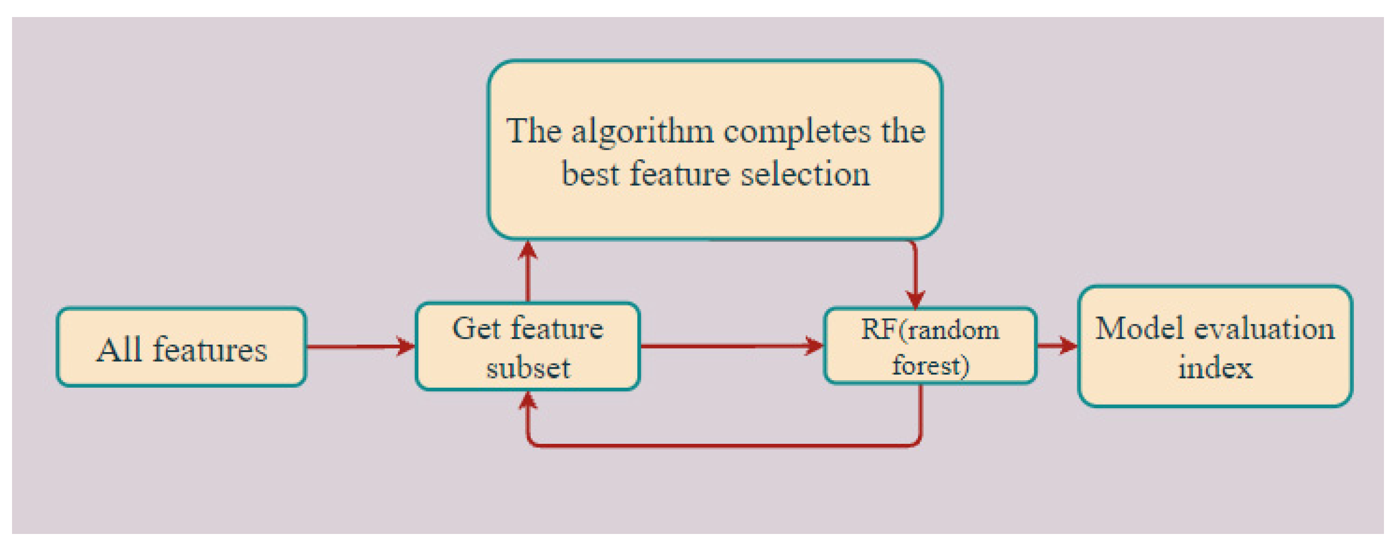
2.5.2. Feature Selection

Random forest recursive feature elimination (RF-RFE) was selected to compare with the feature dimensionality reduction method, it is a wrapping method with the best effect in machine learning. RF-RFE [20] can perform feature selection and algorithm training at the same time. The purpose of optimal band selection is to select wavelengths with small redundancy and collinearity from the full spectra, so as to reduce the data dimension. It is essential to select important features from all features to avoid the situation in which all features are to be imported into the model for training.

Spectral data (104 bands) after two preprocessing methods were taken into the program for feature selection. A random forest classifier is constructed on the initial feature set to rank after obtaining the importance of each feature; then, by pruning the least important features of the current set of features, the process is repeated recursively on the pruned set; finally, the feature set with high classification accuracy is obtained. Figure 5 shows the process of RF-RFE.

2.6. Classification Model

Four supervised machine learning algorithms are chosen. These methods have an excellent performance in the classification model and have a high usage rate in other applications. Decision Tree (DT) is easily understood. It is applicable to all kinds of data and has good performance in solving all kinds of problems. In particular, various integration algorithms with a tree model as the core are widely used in various industries and fields. The disadvantage of DT can be alleviated on the Random Forest Classification (RFC) model. K-Nearest Neighbor (KNN) is the simplest machine learning algorithm. It is widely used in various studies, especially in multi-classification issues. Currently, Support Vector Machine (SVM) is the most powerful machine learning algorithm.

2.6.1. Decision Tree (DT)

Constructed using the recursive top-down model, Decision Tree (DT) [36] is an effective intelligent learning classification method. In the process of spanning the tree structure, the class label of the data is displayed, and each internal node represents the test for the attribute. The branches of the tree show the connection of the input characteristics of the labels that lead to the results. Simultaneously, the branch represents a test output, and each leaf node stores a category label. It can summarize decision rules based on a set of characteristic and labelled data to solve the problem of tea classification in this study.

2.6.2. Random Forest Classification (RFC)

Random Forest classification is an integrated combinatorial classifier and a representative Bagging integration algorithm. All basic evaluators are decision trees. It combines several decision trees in the forest for prediction, so that RFC can be regarded as a strong classifier integrated with many weak classifiers (DT). Generally, RFC has a higher precision than DT.

2.6.3. K-Nearest Neighbor (KNN)

The principle of KNN [42] is to divide the feature vector space using the drive data and take the division result as the final algorithm model. In this study, according to the distances from the test sample points to other sample points, the algorithm sorted the distances in order, selected the K with the smallest distance, compared the tea categories of K, and classified the test sample points into the tea category with the highest proportion among the K.

Following the establishment of the model, the difference in the K can be seen from Tables 1, 2 and 4. The difference in the K is shown by the algorithm. When establishing the classification model, due to the addition of feature dimensional reduction and feature selection, the accuracy of the original algorithm will change. The K presented in the results is the optimal K of the KNN, which is actually based on adjusting its parameters, in order to improve the accuracy of classification.

2.6.4. Support Vector Machine (SVM)

A support vector machine (SVM) [43] is a classifier that classifies data based on supervised learning with parameters. This is an efficient method of discrimination, better than other traditional algorithms [2]. The algorithm is intended to find a maximum margin hyperplane that can separate the data into a predefined class [18]. The SVM uses the kernel function to map data in a high dimensional space that can separate multiple categories. Consequently, the selection and adjustment of the kernel function parameters are essential in the algorithm.

In this study, after experimenting with four kernel functions (include ‘linear’, ’rbf’, ’sigmoid’, and ‘poly’), the ‘poly’ worked best and was selected. The three core parameters, degree, gamma, and coef0 were adjusted to optimize the model to obtain accurate prediction results. The “grid search” was used to select the optimum parameters, and the parameters were optimized by selecting the output with the highest accuracy.

“Poly” kernel function expression:

$$K\left(x,y\right)={\left(r\left(x·y\right)+\gamma \right)}^d$$

(7)

where $\gamma$ = 1.0787, d = 1, and r(coef0) = 0.

2.7. Evaluation Index

In order to evaluate model performance, accuracy is used as an index [44], which is the ratio between number of correct classifications and total samples. The higher the accuracy of the model, the greater the classification effect of the model [45].

The time is that consumed for the classifier. All algorithms in this paper ran on CPU(Intel(R) Core (TM) i5-10210U CPU@ 1.60 GHz), and have been implemented on Python 3.6, the machine learning based on framework scikit-learn 0.24.2.

$$Accuracy=\frac{“\mathit{Number}\mathit{of}\mathit{correct}\mathit{classifications}”}{“\mathit{Total}\mathit{samples}”}\times 100\%$$

(8)

3. Results

3.1. Spectral Preprocessing

In the process of obtaining fluorescence spectrum, due to the influence of the environment and other factors, the collected data will produce noise and affect the subsequent model analysis. MSC, SNV, FD, SD and WT are used for data preprocessing. A variety of classification models are compared to obtain the accuracy by 10 times cross-validation of the model.

Table 1. Detection results based on different models of various preprocessing methods.

Methods	Models of Classification
	DT	RFC	KNN (5)	SVM
RAW	81.82%	78.03%	81.82%	93.18%
MSC	82.58%	88.64%	90.15%	95.45%
SNV	81.82%	87.88%	90.15%	96.21%
FD	84.85%	85.61%	87.12%	92.48%
SD	76.52%	79.55%	86.36%	91.48%
WT	81.82%	75.76%	81.82%	91.67%

and Figure 6 show the results of the accuracy of test sets in different classification models by various preprocessing methods (MSC, SNV, FD, SD and WT) of the raw spectrum respectively.

As shown in Figure 6, the accuracy of the test set after MSC and SNV is the best under various classification models except for the DT, and the test set obtained by RFC, KNN and SVM is higher than that of the other three preprocessing methods. The accuracy of RFC, KNN and SVM using MSC and SNV is not significantly different. Of all preprocessing methods, WT produces the poorest data processing effect, which will affect the accuracy of the model. FD, which is 84.45%, produces the best accuracy on the DT model. The preprocessing method should be used on other classification models, so MSC and SNV are used to explore the follow-up research. Figure 7a,b shows the spectral after MSC and SNV, respectively.

These two methods perform very well in data preprocessing, they both aim to eliminate the scattering effects caused by uneven particle distribution and different particle sizes, so they look alike. The difference is that SNV deals with a single spectral curve, and the fluorescence intensity is treated as a group of curves with a mean value of 0 and a standard deviation of 1. However, MSC processes the spectra of a group of samples to reduce spectral differences and retain as much information of the original spectral as possible [46].

3.2. Characteristic Wavelength Selection

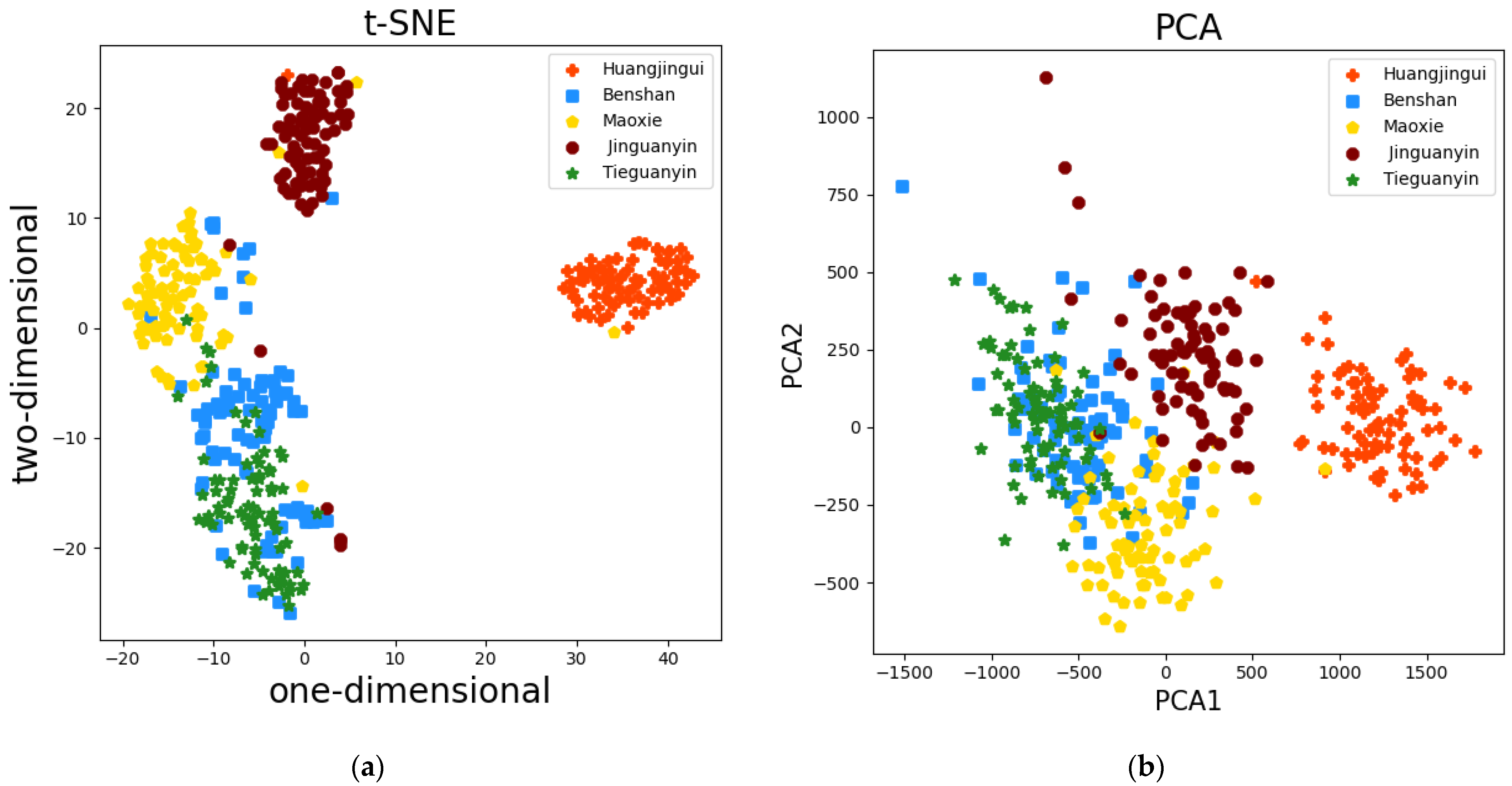
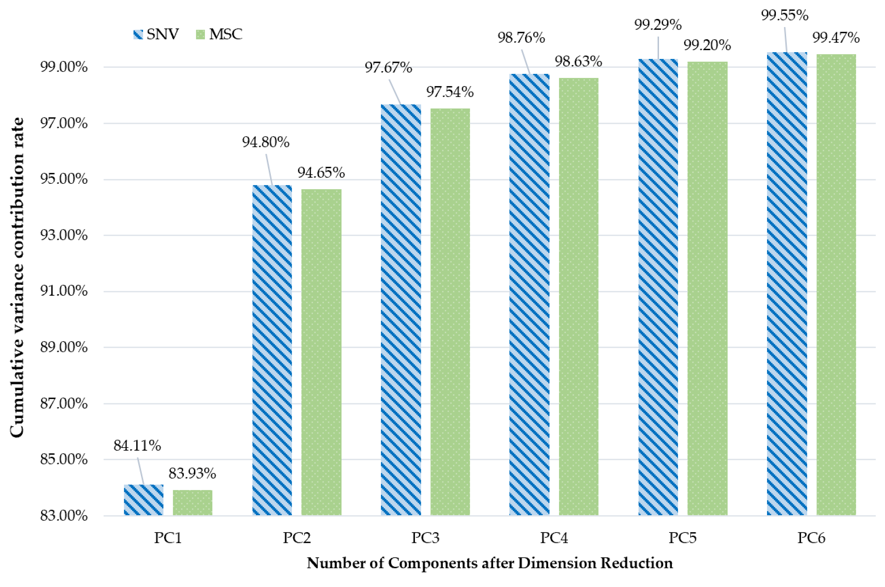
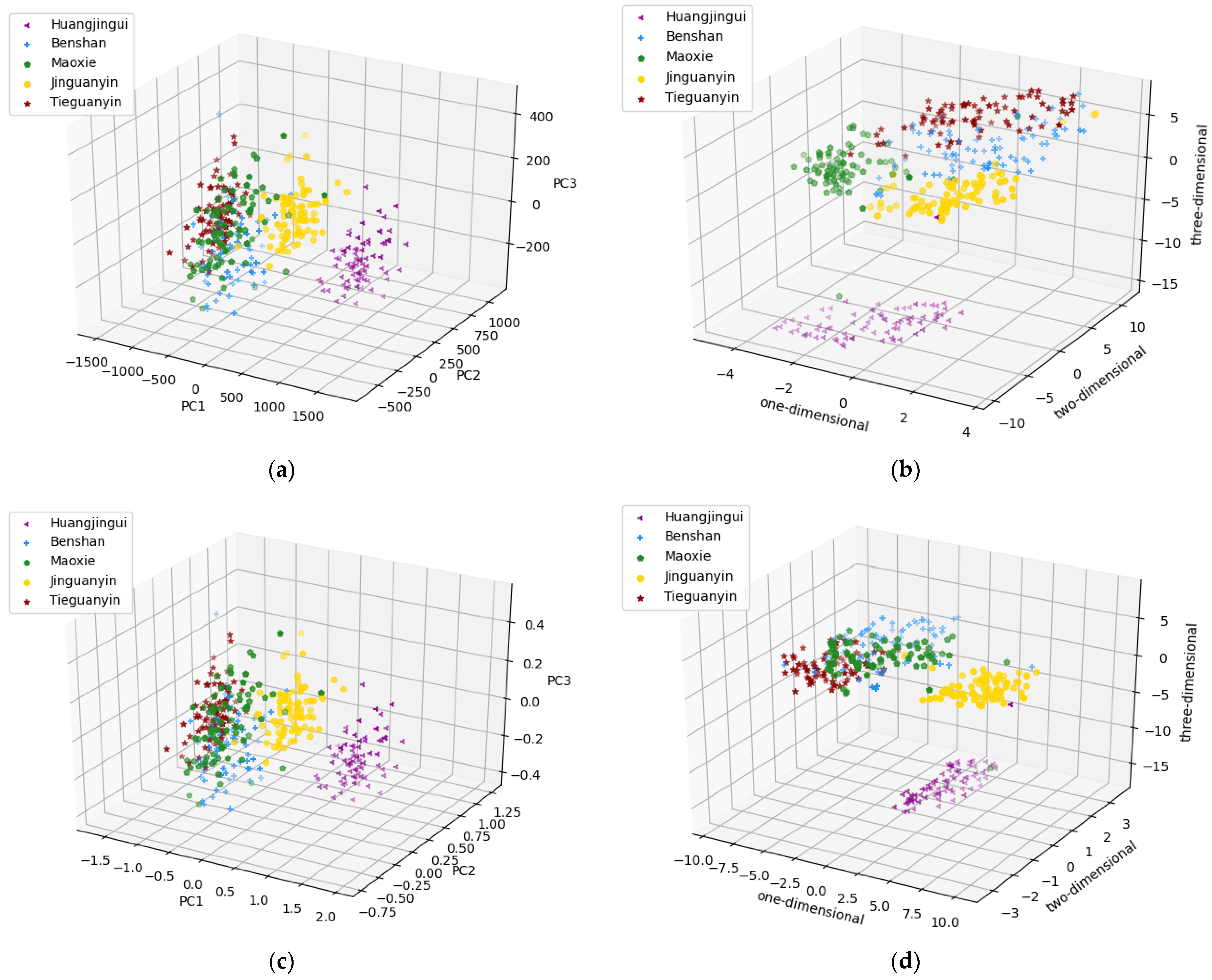
3.2.1. PCA and t-SNE Dimensionality Reduction Algorithm

After preprocessing, there is still a great deal of information not related to the data. Without further extraction of effective information, high dimensional data will undoubtedly affect the accuracy and robustness of the model. As is shown in Figure 8, PCA and t-SNE are used to reduce dimensionality, and data are visually displayed in two dimensions. Both can display five types of Oolong tea in the form of “clusters”. Nonetheless, t-SNE can better display five types of tea as ‘clusters’. From PCA, there are more intersections in Ben and Tie. Through visual display, it is meaningful to classify five types of Oolong tea.

PCA was used to obtain the cumulative contribution rates of the first six principal components after preprocessing, as is shown in Figure 9. After PCA, when the dimensionality is reduced to three dimensions, the data can contain more than 97.5% of the total information. Considering t-SNE, the effect is best when dimensionality is reduced into two or three dimensions. When comparing PCA and t-SNE, the features are both reduced to three dimensions. As is shown in Figure 10a–d, there are visual diagrams of two feature selection methods when reduced to three dimensions. t-SNE can more clearly distinguish different types of tea. There are still more intersections in the PCA, which is similar to the conclusion in the last paragraph.

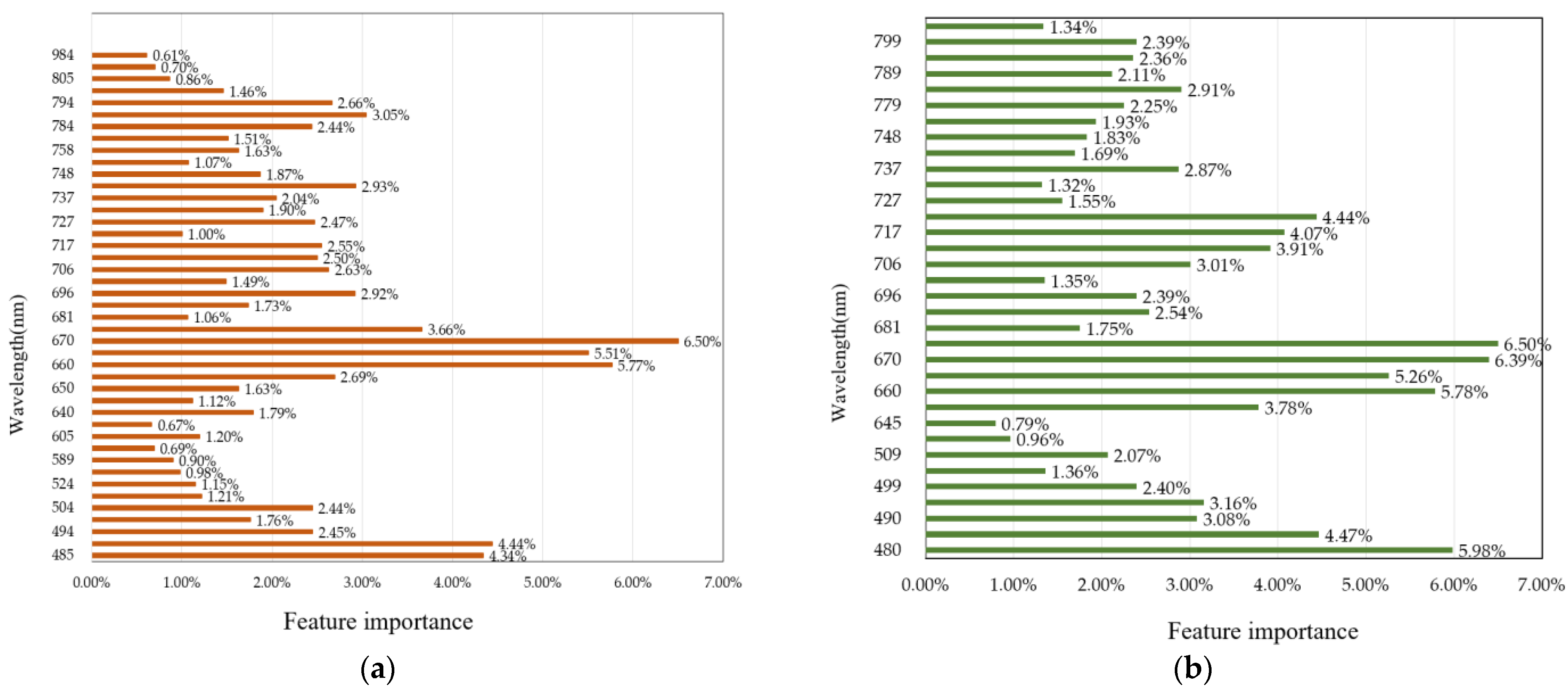
3.2.2. RF-RFE Feature Selection Method

The data collected by fluorescence hyperspectral system contained a large quantity of highly relevant and redundant information. Consequently, the wavelength number was reduced to further process the data. RF-RFE was used to select the wavelength of the origin spectra after two preprocessing methods. The contribution rate for each wavelength is obtained by 10 iterations of cross-validation, and the wavelength with a high contribution rate is selected, as shown in

Table 2. The selected bands after two preprocessing methods combined with RF-RFE.

	Methods	Number	Selected Wavelengths (nm)
RF-RFE	MSC	44	479, 484, 489, 494, 499, 504, 509, 524, 574, 589, 594, 604, 624, 639, 645, 650, 655, 660, 665, 670, 675, 680, 690, 696, 701, 706, 711, 716, 721, 726, 732, 737, 742, 747, 752, 757, 778, 783, 788, 794, 799, 804, 809, 984
	SNV	34	479, 484, 489, 494, 499, 504, 509, 609, 645, 655, 660, 665, 670, 675, 680, 690, 696, 701, 706, 711, 716, 721, 726, 732, 737, 742, 747, 752, 778, 783, 788, 794, 799, 804

. MSC and SNV combined with RF-RFE reduced the 104 raw spectral channels to 44 and 34, respectively. Figure 11a,b shows the proportion of wavelength channels and feature importance after two preprocessing methods in combination with RF-RFE.

Figure 11 shows that the bands chosen by the two preprocessing methods are quite similar. The bands chosen by MSC basically include the bands chosen by SNV. An important feature shared by the two preprocessing methods is that the wavelength is 676 nm, accounting for 6.50%. The important bands are mainly concentrated near the two bands, about 675 nm and 490 nm, respectively, indicating that there is more effective information near the two bands. The importance of the band near 590 nm accounts for less in the selected wavelengths. The experimental results show that under the two preprocessing methods, the overall trend of the selected bands after RF-RFE is similar. Therefore, the bands chosen in the above process are used as input into the following classification model.

3.3. Original Band Classification Results

Table 3. Accuracy and the time of original band classification model.

Model	Method	Train-Accuracy	Test-Accuracy	Time (s)
DT	RAW	87.68%	83.21%	0.0120
RFC	RAW	89.00%	83.33%	0.0898
KNN-7	RAW	89.92%	81.06%	0.0140
SVM	RAW	96.26%	92.42%	0.0050

shows the results of the training set and test set of four classification models obtained from the raw data without preprocessing or feature processing. It reveals that compared with each algorithm on the raw data without preprocessing, the time spent by RFC is 0.0898 s. RFC takes longer but has higher accuracy than DT. The reason for this is that the base evaluator of RFC is DT. RFC is comprised of multiple simple trees and each tree is based on random samples of training data. With the addition of trees, the decision limit becomes more accurate, which is generally more accurate than that of a single decision tree, but it takes longer. The accuracy of DT, RFC and KNN (7) is lower than SVM. SVM has produced the best effect since the training set and test set have the highest accuracy among the four models, 96.26% and 92.42%, respectively, and the least time spent at 0.0050 s.

3.4. Modeling Analysis after Preprocessing and Feature Processing

The accuracy and timing of establishing the classification prediction model using different preprocessing and feature processing methods are shown in

Table 4. Results of various classification models.

Models	Methods	Train-Accuracy	Test-Accuracy	Time (s)
DT	MSC	88.06%	82.58%	0.0030
	SNV	91.79%	84.09%	0.0020
	MSC-RF-RFE (44)	91.04%	89.39%	0.0020
	SNV-RF-RFE (34)	91.79%	87.88%	0.0020
RFC	MSC-PCA	91.79%	85.61%	0.0379
	SNV-PCA	92.16%	86.36%	0.0339
	MSC-TSNE	93.28%	86.36%	0.1606
	SNV-TSNE	93.66%	92.39%	0.1366
	MSC-RF-RFE (44)	93.28%	92.42%	0.0688
	SNV-RF-RFE (34)	91.04%	87.12%	0.0738
KNN (9)	MSC-PCA	85.45%	84.85%	0.0160
	SNV-PCA	85.45%	84.85%	0.0140
	MSC-TSNE	89.93%	87.12%	0.0160
	SNV-TSNE	88.06%	87.12%	0.0160
	MSC-RF-RFE (44)	94.03%	92.42%	0.0205
	SNV-RF-RFE (34)	94.40%	93.94%	0.0160
SVM (poly)	MSC-PCA	97.01%	98.48%	0.0050
	SNV-PCA	97.76%	98.48%	0.0060
	MSC-TSNE	97.31%	96.36%	0.0110
	SNV-TSNE	98.81%	95.09%	0.0110
	MSC-RF-RFE (44)	100.00%	98.73%	0.0040
	SNV-RF-RFE (34)	100.00%	98.21%	0.0030

. In this study, 400 samples were divided into training and test set according to 3:1.

It can be seen from Table 4:

(a) In this study, supervised classification models are used to test the accuracy and time of the optimum Oolong tea model. After preprocessing and feature processing, the accuracy of the model is higher than that by the raw spectral modeling, the dimensionality is reduced, the modeling accuracy is improved to a certain extent, and the robustness is enhanced.

(b) The accuracy of the experimental results indicates that there is a significant discrepancy between the influence of different models. The accuracy of DT and RFC training set is about 90%, while the accuracy of the test set is less than 90%. Improving the accuracy of the DT could result in over-fitting. After cross-validation and grid search, the over-fitting problem still existed. DT’s learning is based on a greedy algorithm and relies on optimizing the local optimal nodes to achieve the overall optimization, which doesn’t guarantee to return the global optimal results. Thus, DT does not fit the tea classification in this study. The disadvantage of DT can be solved on RFC that is randomly sampled into the branching process. The accuracy of RFC on t-SNE and RF-RFE is improved and is not affected by its base evaluator DT. When the data are reduced to three dimensions after SNV-t-SNE-RFC, the model is more accurate than other preprocessing methods. The accuracy of the training set is 93.66% and that of the test set is 92.39%. The KNN has a higher accuracy than the DT and RFC. The accuracy of the training set selected by SNV-RF-RFE-KNN is 94.40% and the test set is 93.94%. Using the MSC-RF-RFE-KNN, the accuracy of the training set is 94.03% and the test set is 92.42%. The two preprocessing methods combined with RF-RFE are helpful to improve KNN’s accuracy. SVM has obvious advantages for the classification of tea in this study. After using SVM, the accuracy of different preprocessing and feature processing methods are higher than that of the other three classification models. Especially in MSC-RF-RFE-SVM, the accuracy of the training set and test set is 100% and 98.73%, respectively, which further underlines the feasibility of SVM in tea classification.

(c) In terms of time, it can be seen that DT spends the least time but has a relatively low accuracy. As for RFC, the time is higher than that of DT, but the accuracy is improved. KNN’s time is similar to that of RFC, but the accuracy is improved. SVM is the most accurate and spends less time.

(d) Among all feature processing methods, the accuracy of t-SNE in the RFC model has been greatly improved. In other classification models, while t-SNE has higher accuracy than PCA, it involves multiple conditional probability and gradient descent calculations. The time and space complexity are quadratic, computer complexity is very high, and it takes more time-consuming than PCA in large data sets. Theoretically, PCA is a matrix decomposition technology, and t-SNE is a probability method. Due to the high computation cost of t-SNE, the computation speed of PCA is faster than that of t-SNE in the same order of magnitude. Additionally, a feature selection method is sought. RF-RFE is used to select the best feature band. It has higher accuracy than feature dimensionality reduction methods and takes less time.

In this study, the best model for classifying Oolong tea is MSC-RF-RFE-SVM. Figure 12 shows the confusion matrix under the best method. The classification of the training set is all correct. Huang and Ben are classified correctly, one error occurs respectively when classifying Mao, Jin, and Tie, but the overall classification effect is the best.

4. Conclusions

The results of this study show that fluorescence hyperspectral technology and machine learning are achievable for the nondestructive detection and classification of Oolong tea.

• SNV and MSC can reduce the impact of spectral baseline drift and tilt, and improve the accuracy of the model.
• Feature dimensionality reduction and feature selection can reduce the degree of data redundancy and improve the predictive accuracy and robustness of the model. In the comparison of two feature dimensionality reduction methods and one feature selection method, PCA < t-SNE < RF-RFE.
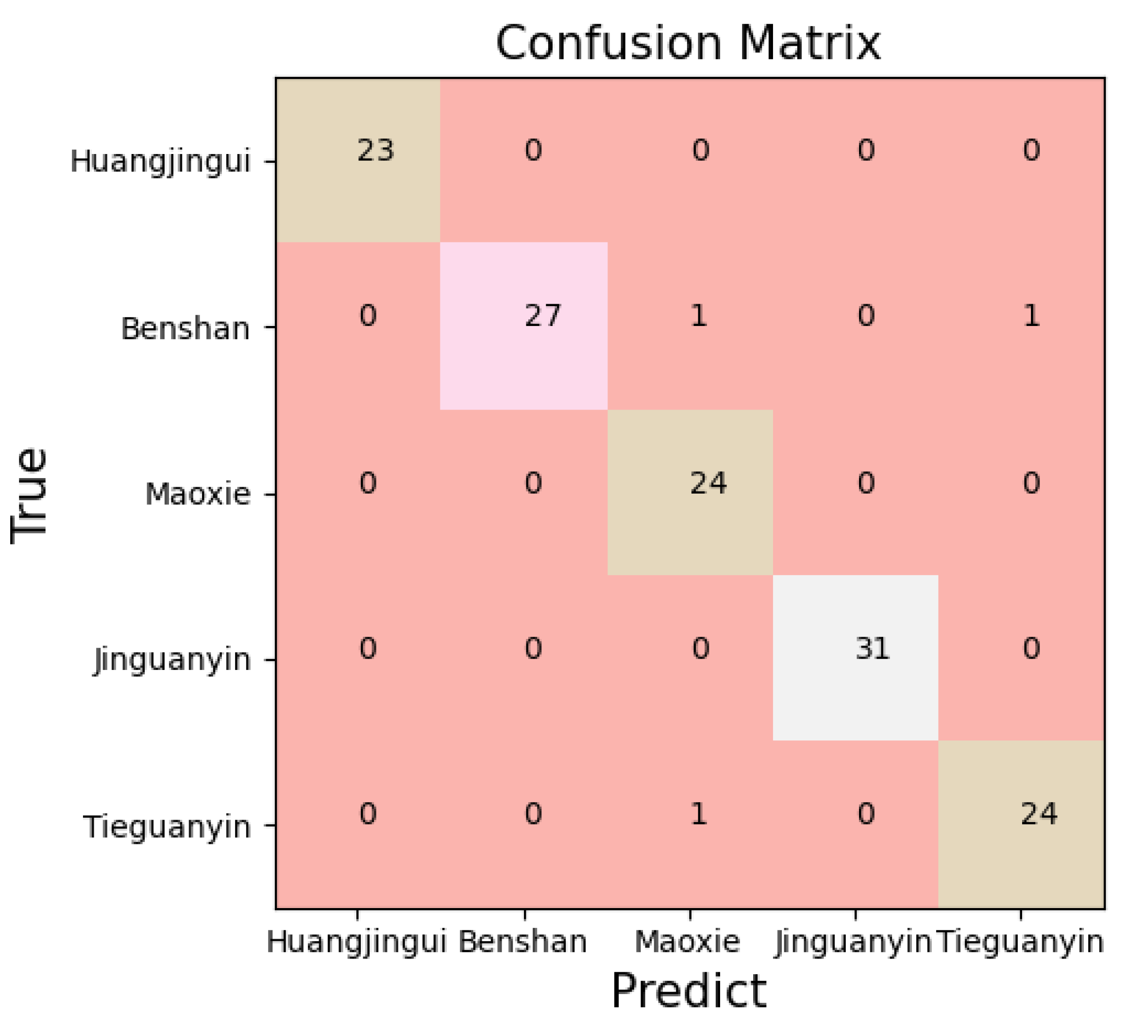
• Among the four classification models, the effect of SVM is the best. SVM combined with preprocessing and feature processing offers the best performance. MSC-RF-RFE-SVM is the best method. The accuracy of the training set and test set reaches 100% and 98.73%, respectively. The accuracy is greater than other spectroscopy and chemical methods.

Currently, identifying tea is still a long and laborious process. Fluorescence hyperspectral technology is a rapid and nondestructive testing method, but is scarcely used in real life. In this study, the feasibility of fluorescence hyperspectral technology and machine learning in the detection of Oolong tea species has been demonstrated. In the future, our research group will make improvements in the following aspects: 1. Continue to study the application of fluorescence hyperspectral technology in nondestructive testing fields. 2. Miniaturized equipment will be produced and applied to tea classification. 3. Based on the results of in this study, the detection of adulteration in Oolong tea will be investigated further. We hope that our research will be able to refer the identification and classification of other agricultural products.

References

1. Luo, X.; Xu, L.; Huang, P.; Wang, Y.; Liu, J.; Hu, Y.; Wang, P.; Kang, Z. Nondestructive Testing Model of Tea Polyphenols Based on Hyperspectral Technology Combined with Chemometric Methods. Agriculture 2021, 11, 673. [Google Scholar] [CrossRef]
2. Ahmad, H.; Sun, J.; Nirere, A.; Shaheen, N.; Zhou, X.; Yao, K. Classification of tea varieties based on fluorescence hyperspectral image technology and ABC-SVM algorithm. J. Food Process. Preserv. 2021, 45, e15241. [Google Scholar] [CrossRef]
3. Ning, J.M.; Sun, J.J.; Li, S.H.; Sheng, M.G.; Zhang, Z.Z. Classification of five Chinese tea categories with different fermentation degrees using visible and near-infrared hyperspectral imaging. Int. J. Food Prop. 2017, 20, 1515–1522. [Google Scholar] [CrossRef] [Green Version]
4. Chen, G.; Zhang, X.; Wu, Z.; Su, J.; Cai, G. An efficient tea quality classification algorithm based on near infrared spectroscopy and random Forest. J. Food Process Eng. 2020, 44, e13604. [Google Scholar] [CrossRef]
5. Ren, G.; Liu, Y.; Ning, J.; Zhang, Z. Assessing black tea quality based on visible–near infrared spectra and kernel-based methods. J. Food Compos. Anal. 2021, 98, 103810. [Google Scholar] [CrossRef]
6. Li, M.; Pan, T.; Chen, Q. Estimation of tea quality grade using statistical identification of key variables. Food Control 2021, 119, 107485. [Google Scholar] [CrossRef]
7. Yu, X.-L.; He, Y. Fast nondestructive identification of steamed green tea powder adulterations in matcha by visible spectroscopy combined with chemometrics. Spectrosc. Lett. 2018, 51, 112–117. [Google Scholar] [CrossRef]
8. Wang, Y.; Li, M.; Li, L.; Ning, J.; Zhang, Z. Green analytical assay for the quality assessment of tea by using pocket-sized NIR spectrometer. Food Chem. 2021, 345, 128816. [Google Scholar] [CrossRef]
9. Yang, J.; Wang, J.; Lu, G.; Fei, S.; Yan, T.; Zhang, C.; Lu, X.; Yu, Z.; Li, W.; Tang, X. TeaNet: Deep learning on Near-Infrared Spectroscopy (NIR) data for the assurance of tea quality. Comput. Electron. Agric. 2021, 190, 106431. [Google Scholar] [CrossRef]
10. Wang, P.; Liu, J.; Xu, L.; Huang, P.; Luo, X.; Hu, Y.; Kang, Z. Classification of Amanita Species Based on Bilinear Networks with Attention Mechanism. Agriculture 2021, 11, 393. [Google Scholar] [CrossRef]
11. Dong, C.; Ye, Y.; Yang, C.; An, T.; Jiang, Y.; Ye, Y.; Li, Y.; Yang, Y. Rapid detection of catechins during black tea fermentation based on electrical properties and chemometrics. Food Biosci. 2021, 40, 100855. [Google Scholar] [CrossRef]
12. Wang, Y.; Li, L.; Liu, Y.; Cui, Q.; Ning, J.; Zhang, Z. Enhanced quality monitoring during black tea processing by the fusion of NIRS and computer vision. J. Food Eng. 2021, 304, 110599. [Google Scholar] [CrossRef]
13. Yuan, L.M.; Mao, F.; Huang, G.; Chen, X.; Wu, D.; Li, S.; Zhou, X.; Jiang, Q.; Lin, D.; He, R. Models fused with successive CARS-PLS for measurement of the soluble solids content of Chinese bayberry by vis-NIRS technology. Postharvest Biol. Technol. 2020, 169, 111308. [Google Scholar] [CrossRef]
14. Li, X.; Li, Z.; Yang, X.; He, Y. Boosting the generalization ability of Vis-NIR-spectroscopy-based regression models through dimension reduction and transfer learning. Comput. Electron. Agric. 2021, 186, 106157. [Google Scholar] [CrossRef]
15. Li, L.; Huang, J.; Wang, Y.; Jin, S.; Li, M.; Sun, Y.; Ning, J.; Chen, Q.; Zhang, Z. Intelligent evaluation of storage period of green tea based on VNIR hyperspectral imaging combined with chemometric analysis. Infrared Phys. Technol. 2020, 110, 103450. [Google Scholar] [CrossRef]
16. Cardoso, V.G.K.; Poppi, R.J. Non-invasive identification of commercial green tea blends using NIR spectroscopy and support vector machine. Microchem. J. 2021, 164, 106052. [Google Scholar] [CrossRef]
17. Zhao, J.W.; Chen, Q.S.; Cai, J.R.; Ouyang, Q. Automated tea quality classification by hyperspectral imaging. Appl. Opt. 2009, 48, 3557–3564. [Google Scholar] [CrossRef] [PubMed]
18. Zhang, X.; Sun, J.; Li, P.; Zeng, F.; Wang, H. Hyperspectral detection of salted sea cucumber adulteration using different spectral preprocessing techniques and SVM method. LWT 2021, 152, 112295. [Google Scholar] [CrossRef]
19. Hong, Z.; Zhang, C.; Kong, D.; Qi, Z.; He, Y. Identification of storage years of black tea using near-infrared hyperspectral imaging with deep learning methods. Infrared Phys. Technol. 2021, 114, 103666. [Google Scholar] [CrossRef]
20. Sun, J.; Zhang, Y.; Mao, H.; Cong, S.; Wu, X.; Wang, P. Research of moldy tea identification based on RF-RFE-Softmax model and hyperspectra. Opt.-Int. J. Light Electron. Opt. 2018, 153, 156–163. [Google Scholar] [CrossRef]
21. Wang, H.; Wan, X. Effect of chlorophyll fluorescence quenching on quantitative analysis of adulteration in extra virgin olive oil. Spectrochim. Acta A Mol. Biomol. Spectrosc. 2021, 248, 119183. [Google Scholar] [CrossRef]
22. Liu, Y.; Zou, J.; Luo, B.; Yu, H.; Zhao, Z.; Xia, H. Ivy extract-assisted photochemical vapor generation for sensitive determination of mercury by atomic fluorescence spectrometry. Microchem. J. 2021, 169, 106547. [Google Scholar] [CrossRef]
23. Guo, X.J.; He, X.S.; Li, C.W.; Li, N.X. The binding properties of copper and lead onto compost-derived DOM using Fourier-transform infrared, UV-vis and fluorescence spectra combined with two-dimensional correlation analysis. J. Hazard. Mater. 2019, 365, 457–466. [Google Scholar] [CrossRef]
24. Li, G.; Liao, Y.; Wang, X.; Sheng, S.; Yin, D. In situ estimation of the entire color and spectra of age pigment-like materials: Application of a front-surface 3D-fluorescence technique. Exp. Gerontol. 2006, 41, 328–336. [Google Scholar] [CrossRef]
25. Hu, Y.; Zhang, H.; Zhao, D. Transform method in three-dimensional fluorescence spectra for direct reflection of internal molecular properties in rapid water contaminant analysis. Spectrochim. Acta A Mol. Biomol. Spectrosc. 2021, 250, 119376. [Google Scholar] [CrossRef]
26. Sunuwar, S.; Manzanares, C.E. Excitation, emission, and synchronous fluorescence for astrochemical applications: Experiments and computer simulations of synchronous spectra of polycyclic aromatic hydrocarbons and their mixtures. Icarus 2021, 370, 114689. [Google Scholar] [CrossRef]
27. Zhou, X.; Sun, J.; Tian, Y.; Yao, K.; Xu, M. Detection of heavy metal lead in lettuce leaves based on fluorescence hyperspectral technology combined with deep learning algorithm. Spectrochim. Acta A Mol. Biomol. Spectrosc. 2021, 266, 120460. [Google Scholar] [CrossRef] [PubMed]
28. Yu, Y.; Qu, Y.; Zhang, M.; Guo, X.; Zhang, H. Fluorescence detection of paclobutrazol pesticide residues in apple juice. Optik 2020, 224, 165542. [Google Scholar] [CrossRef]
29. Lim, C.M.; Carey, M.; Williams, P.N.; Koidis, A. Rapid classification of commercial teas according to their origin and type using elemental content with X-ray fluorescence (XRF) spectroscopy. Curr. Res. Food Sci. 2021, 4, 45–52. [Google Scholar] [CrossRef]
30. Wang, Y.-J.; Jin, G.; Li, L.-Q.; Liu, Y.; Kalkhajeh, Y.K.; Ning, J.-M.; Zhang, Z.-Z. NIR hyperspectral imaging coupled with chemometrics for nondestructive assessment of phosphorus and potassium contents in tea leaves. Infrared Phys. Technol. 2020, 108, 103365. [Google Scholar] [CrossRef]
31. Wei, X.; He, J.; Zheng, S.; Ye, D. Modeling for SSC and firmness detection of persimmon based on NIR hyperspectral imaging by sample partitioning and variables selection. Infrared Phys. Technol. 2020, 105, 103099. [Google Scholar] [CrossRef]
32. Zhao, Y.; Zhang, C.; Zhu, S.; Li, Y.; He, Y.; Liu, F. Shape induced reflectance correction for non-destructive determination and visualization of soluble solids content in winter jujubes using hyperspectral imaging in two different spectral ranges. Postharvest Biol. Technol. 2020, 161, 111080. [Google Scholar] [CrossRef]
33. Zhu, X.; Li, W.; Wu, R.; Liu, P.; Hu, X.; Xu, L.; Xiong, Z.; Wen, Y.; Ai, S. Rapid detection of chlorpyrifos pesticide residue in tea using surface-enhanced Raman spectroscopy combined with chemometrics. Spectrochim. Acta A Mol. Biomol. Spectrosc. 2021, 250, 119366. [Google Scholar] [CrossRef] [PubMed]
34. Song, Y.; Wang, X.; Xie, H.; Li, L.; Ning, J.; Zhang, Z. Quality evaluation of Keemun black tea by fusing data obtained from near-infrared reflectance spectroscopy and computer vision sensors. Spectrochim. Acta A Mol. Biomol. Spectrosc. 2021, 252, 119522. [Google Scholar] [CrossRef]
35. Zhang, D.; Zhao, Z.; Zhang, S.; Chen, F.; Sheng, Z.; Deng, F.; Zeng, Q.; Guo, L. Accurate identification of soluble solid content in citrus by indirect laser-induced breakdown spectroscopy with its leaves. Microchem. J. 2021, 169, 106530. [Google Scholar] [CrossRef]
36. Xia, Y.; Fan, S.; Tian, X.; Huang, W.; Li, J. Multi-factor fusion models for soluble solid content detection in pear (Pyrus bretschneideri ‘Ya’) using Vis/NIR online half-transmittance technique. Infrared Phys. Technol. 2020, 110, 103443. [Google Scholar] [CrossRef]
37. Jamwal, R.; Amit; Kumari, S.; Sharma, S.; Kelly, S.; Cannavan, A.; Singh, D.K. Recent trends in the use of FTIR spectroscopy integrated with chemometrics for the detection of edible oil adulteration. Vib. Spectrosc. 2021, 113, 103222. [Google Scholar] [CrossRef]
38. Huang, Y.; Dong, W.; Sanaeifar, A.; Wang, X.; Luo, W.; Zhan, B.; Liu, X.; Li, R.; Zhang, H.; Li, X. Development of simple identification models for four main catechins and caffeine in fresh green tea leaf based on visible and near-infrared spectroscopy. Comput. Electron. Agric. 2020, 173, 105388. [Google Scholar] [CrossRef]
39. Bunaciu, A.A.; Aboul-Enein, H.Y. Adulterated drug analysis using FTIR spectroscopy. Appl. Spectrosc. Rev. 2020, 56, 423–437. [Google Scholar] [CrossRef]
40. Wang, S.; Liu, S.; Yuan, Y.; Zhang, J.; Wang, Z.; Che, X. A novel CC-tSNE-SVR model for rapid determination of diesel fuel quality by near infrared spectroscopy. Infrared Phys. Technol. 2020, 106, 103276. [Google Scholar] [CrossRef]
41. Ndlovu, P.F.; Magwaza, L.S.; Tesfay, S.Z.; Mphahlele, R.R. Rapid spectroscopic method for quantifying gluten concentration as a potential biomarker to test adulteration of green banana flour. Spectrochim. Acta A Mol. Biomol. Spectrosc. 2021, 262, 120081. [Google Scholar] [CrossRef] [PubMed]
42. Xie, C.; Lee, W.S. Detection of citrus black spot symptoms using spectral reflectance. Postharvest Biol. Technol. 2021, 180, 111627. [Google Scholar] [CrossRef]
43. Yao, M.; Fu, G.; Chen, T.; Liu, M.; Xu, J.; Zhou, H.; He, X.; Huang, L. A modified genetic algorithm optimized SVM for rapid classification of tea leaves using laser-induced breakdown spectroscopy. J. Anal. At. Spectrom. 2021, 36, 361–367. [Google Scholar] [CrossRef]
44. Wei, X.; He, J.-C.; Ye, D.-P.; Jie, D.-F. Navel Orange Maturity Classification by Multispectral Indexes Based on Hyperspectral Diffuse Transmittance Imaging. J. Food Qual. 2017, 2017, 1023498. [Google Scholar] [CrossRef] [Green Version]
45. Firmani, P.; De Luca, S.; Bucci, R.; Marini, F.; Biancolillo, A. Near infrared (NIR) spectroscopy-based classification for the authentication of Darjeeling black tea. Food Control 2019, 100, 292–299. [Google Scholar] [CrossRef]
46. Huang, Y.; Dong, W.; Chen, Y.; Wang, X.; Luo, W.; Zhan, B.; Liu, X.; Zhang, H. Online detection of soluble solids content and maturity of tomatoes using Vis/NIR full transmittance spectra. Chemom. Intell. Lab. Syst. 2021, 210, 104243. [Google Scholar] [CrossRef]
Figure 1. Fluorescence hyperspectral system.
Agriculture 11 01106 g001
Figure 2. Fluorescence hyperspectral image of tea.
Agriculture 11 01106 g002
Figure 3. Extraction of fluorescence spectra information of tea.
Agriculture 11 01106 g003
Figure 4. Raw spectra of tea.
Agriculture 11 01106 g004
Figure 5. Process of RF-RFE.
Agriculture 11 01106 g005
Figure 6. Results based on different models of various preprocessing methods.
Agriculture 11 01106 g006
Figure 7. Two preprocessing methods. (a) Spectra after MSC; (b) Spectra after SNV.
Agriculture 11 01106 g007
Figure 8. Diagrams reduced to two dimensions. (a) The visual display of t-SNE (b) The visual display of PCA.
Agriculture 11 01106 g008
Figure 9. Principal component cumulative contribution after SNV and MSC.
Agriculture 11 01106 g009
Figure 10. Visual diagrams of two feature selection methods when reduced to three dimensions (a) MSC-PCA, (b) MSC-t-SNE, (c) SNV-PCA, (d) SNV-t-SNE.
Agriculture 11 01106 g010
Figure 11. Feature bands selected by different algorithms. (a) MSC-RF-RFE, (b) SNV-RF-RFE.
Agriculture 11 01106 g011
Figure 12. Confusion matrix of MSC-RF-RFE-SVM (The diagonal number is the number of correctly classified tea varieties).
Agriculture 11 01106 g012