
Identification of Geographical Origin of Chinese Chestnuts Using Hyperspectral Imaging with 1D-CNN Algorithm


College of Mechanical and Electronic Engineering, Nanjing Forestry University, Nanjing 210037, China
*
Author to whom correspondence should be addressed.
Agriculture 2021, 11(12), 1274; https://0-doi-org.brum.beds.ac.uk/10.3390/agriculture11121274
Submission received: 8 November 2021
/
Revised: 3 December 2021
/
Accepted: 14 December 2021
/
Published: 15 December 2021
(This article belongs to the Special Issue Sensors Applied to Agricultural Products)
Abstract
:The adulteration in Chinese chestnuts affects the quality, taste, and brand value. The objective of this study was to explore the feasibility of the hyperspectral imaging (HSI) technique to determine the geographical origin of Chinese chestnuts. An HSI system in spectral range of 400–1000 nm was applied to identify a total of 417 Chinese chestnuts from three different geographical origins. Principal component analysis (PCA) was preliminarily used to investigate the differences of average spectra of the samples from different geographical origins. A deep-learning-based model (1D-CNN, one-dimensional convolutional neural network) was developed first, and then the model based on full spectra and optimal wavelengths were established for various machine learning methods, including partial least squares-discriminant analysis (PLS-DA) and particle swarm optimization-support vector machine (PSO-SVM). The optimal results based on full spectra for 1D-CNN, PLS-DA, and PSO-SVM models were 97.12%, 97.12%, and 95.68%, respectively. Competitive adaptive reweighted sampling (CARS) and a successive projections algorithm (SPA) were individually utilized for wavelengths selection, and the results of simplified models generally improved. The contrasting results demonstrated that the prediction accuracies of SPA-PLS-DA and 1D-CNN both reached 97.12%, but 1D-CNN presented a higher Kappa coefficient value than SPA-PLS-DA. Meanwhile, the sensitivities and specificities of SPA-PLS-DA and 1D-CNN models were both above 90% for the samples from each geographical origin. These results indicated that both SPA-PLS-DA and 1D-CNN models combined with HSI have great potential for the geographical origin identification of Chinese chestnuts.
1. Introduction
The chestnut (Castanea mollissima Blume.), originating from China, has a planting history of more than 3000 years [1]. Chestnut fruit is rich in nutrients (such as protein, fatty acids, and carbohydrates), vitamins, and minerals, and is widely planted in Asia, Europe, and Africa. Moreover, chestnut fruit has a certain medicinal value. It can be developed as gluten-free food to treat coeliac disease caused by intolerance to peptides derived from the digestion of the cereal protein gluten [2,3]. The high nutrient and medical value have resulted in an important chestnut market.
According to the statistics of the Food and Agriculture Organization of the United Nations (FAO), the planting area and output of Chinese chestnut in China have ranked first since 2007, of which the output accounts for more than 80% of the world. In 2019, the Chinese chestnut planting area was 330,000 hectares, and the output reached 1.84 million tons [4]. Chinese chestnut has been traditionally divided into five groups (Yangtze River Basin, Northern China, Northwestern China, Southeastern China, and Southwestern China) [5]. Due to the differences in longitude, latitude, and climate, there are great differences in the quality, taste, and brand value of the Chinese chestnuts from different planting areas. Inevitably, this difference may lead to fraud, such as mislabeling the origin to cover up the original origin. Therefore, it is significant for both producers and consumers to effectively identify the geographical origin of Chinese chestnuts.
In general, several techniques have been applied to determine the geographical origin of chestnuts, such as high-performance liquid chromatography (HPLC) [6], gas chromatography-mass spectrometer (GC-MS) [7,8], nuclear magnetic resonance (NMR) [9,10], X-ray diffraction [10,11], etc. However, these techniques are time-consuming, expensive, or destructive. In addition, these techniques often require professional laboratories, which means that they are difficult to be apply to large-scale online detection.
In recent years, the computer vision technique has been widely concerned as a rapid and non-destructive one [12]. However, this technique is only effective in identifying samples with apparent appearance characteristics, and cannot be used to distinguish the internal differences of samples. As an internal detection technique, near-infrared spectroscopy (NIRS) has been widely used to identify the geographical and botanical origin of agricultural products [13], particularly nuts, e.g., hazelnut [14,15,16], macadamia nut [17], walnut [18,19], and pine nut [20]. However, NIRS cannot obtain the information in the whole sample space due to single-point detection [21].
The hyperspectral imaging (HSI) is a technique which organically integrates spatial image information and spectral information [22]. In contrast to NIRS, HSI technique provides a piece of three-dimensional hypercube information and obtains a wide range of chemical information from the sample. Therefore, HSI has a more comprehensive interpretation for the whole sample, which is conducive in discriminating different geographical origins of agricultural products. In this context, HSI has been widely adopted in the field of agricultural products, including fruits [23], cereals [24,25,26], meats [27], vegetables [28], and seafoods [29]. Additionally, the HSI technique was also often used to screen discolored [30,31], immature [32,33], moldy [34], and insect damage samples [35]. In terms of chestnut, HSI has been applied to distinguish moldy samples [36]. To our knowledge, little research related to determining the geographical origin of chestnuts using HSI has been documented so far.
In this study, HSI was combined with partial least squares-discriminant analysis (PLS-DA), particle swarm optimization-support vector machine (PSO-SVM), and the deep learning modeling methods based on convolutional neural network (CNN) to distinguish the geographical origin of Chinese chestnuts. Furthermore, the accuracies and efficiencies of different modeling algorithms were compared. To improve the robustness of the modeling results, different preprocessings and wavelength selection methods were also attempted and compared. Finally, the classification results of the optimal model were chosen to discriminate the geographical origin of Chinese chestnuts.
2. Materials and Methods
2.1. Sample Preparation
The geographical origins of Chinese chestnut samples in this experiment were Qianxi (Hebei province, China), Dandong (Liaoning province, China), and Yuxi (Yunnan province, China). To guarantee the authenticity of samples, chestnuts were purchased directly from farmers in the three different geographical areas in 2020. In detail, Qianxi chestnuts were collected from Han Erzhuang village, Qianxi county, Tangshan city (40°21′ N, 118°13′ E); Dandong chestnuts were collected from Taoli village, Dongtang county, Dandong city (40°28′ N, 124°18′ E); and Yuxi chestnuts were collected from Pubei village, Yimen county, Yuxi city (24°33′ N, 102°12′ E). After collection, these chestnut samples were stored at 0–4 °C. Before the spectra collection, chestnuts need to be kept at room temperature of about 24 °C for 2 h to achieve temperature balance [37]. The total number of samples involved in the experiment was 417, including 144 Qianxi samples, 129 Dandong samples, and 144 Yuxi samples. Then, the calibration set and prediction set were divided based on a ratio of 2:1, with 278 samples (including 96 Qianxi chestnuts, 86 Dandong chestnuts, and 96 Yuxi chestnuts) used for establishing classification models, and the remaining 139 samples (including 48 Qianxi chestnuts, 43 Dandong chestnuts, and 48 Yuxi chestnuts) were used for external validation of the developed models. In order to select the representative learning samples, the Kennard–Stone (K–S) algorithm was assayed to divide the sample sets, which calculated the difference between samples according to the Euclidean distance between samples and iterated out the most representative samples as the calibration set. The K–S algorithm was conducted in Matlab 2017b software (The MathWorks Inc., Natick, MA, USA).
2.2. Hyperspectral Image Acquisition and Correction
The hyperspectral images were obtained by the “GaiaSorter” hyper-spectrometer produced by Zolix Instruments Co., Ltd. (Beijing, China), working in range of 383.4 nm to 990.4 nm. The push-broom line-scan hyper-spectrometer was equipped with CCD (Imperx Inc., Boca Raton, FL, USA), V10 imaging spectrometer (Spectral Imaging Ltd., Qulu, Finland), 45 W halogen lamp (Osram GmbH, Munich, Germany), electrically controlled displacement table (100–200 mm/s), and other accessories. In addition, the pixel resolution of this spectrometer is 0.63 nm, and the number of pixels in full image is 1392 × 1040. Finally, hyperspectral images collected by SpecView (SpecView Ltd., Uckfield, UK) software contain 176 channels with a nominal resolution (the best resolution) of 3.2 nm.
Before the hyperspectral images acquisition, the original image (R) needs to be calibrated in black and white to reduce the dark current of the CCD camera and the influence of environmental factors. White calibration images (W) were obtained by taking a spectral image of white Teflon (Gilden Photonics Ltd., Glasgow, UK) with a reflectivity close to 100%, and black calibration images (B) were obtained by taking a hyperspectral image with all light sources turned off and an opaque black lens cap completely closed. After two calibration graphs were collected, the correction image (C) was calculated according to the following formula:
2.3. Region of Interest (ROI) Identification
The original hyperspectral image contains information of both chestnuts and background. ROI was used to remove the background to extract spectral data of only the pure chestnut samples. ENVI Vision 5.3 software (Research Systems Inc., Boulder, CO, USA) was used to extract the data in our study, and the detailed steps are shown in Figure 1. The original data of hyperspectral images were three-dimensional, with 700 pixels in the X direction, 1000 pixels in the Y direction and 176 bands in the Z direction (383.4–990.4 nm). A total of eight chestnut samples were included in one hyperspectral image. Firstly, the image was resized into eight individual chestnut subsets. Secondly, images with the highest and lowest reflectance at two characteristic bands (band 141 and band 21) were chosen. Then, a grayscale image was prepared by subtracting the image at band 21 from that at band 141. Next, a binary image was generated by setting a threshold value of 0.1 on the grayscale image. The threshold value was preliminarily determined by gray histogram, and then the gray value of chestnut body, edge and background was checked by quick data to find a more accurate threshold in ENVI software. After the above steps, the pixels with values greater than 0.1 were covered in red. After that, the red region was further operated by expansion and corrosion (open operation) to remove burrs and background noise. Finally, the resulting region was used as an ROI, to be further applied to build a mask.
The experimental object of this paper was the chestnut, so the extracted ROI was the cube region composed of the pixels where the chestnut was located, and then the average spectrum of all pixels in the ROI region was obtained. Meanwhile, all average spectra were stored as a data matrix (X). In this paper, there were 417 samples and 176 spectral variables, so the stored data was in the form of a 417 × 176 matrix, where the row vector displayed the sample numbers and the column vector indicated spectral variables. In addition, the labels of origin (Y) were distinguished by 0, 1, and 2, and the data form was 417 × 1.
2.4. Chemometric Methods
2.4.1. Principal Component Analysis
Unsupervised principal component analysis (PCA) is a multivariate statistical method for reducing the dimensionality of multiple variables, avoiding the problems of multi-collinearity or handling potential co-linearity. The main ideal of PCA is to decompose raw spectra into brand new orthogonal variables by maximizing the sample variance. These new orthogonal variables are termed principal components (PCs). Typically, the first few PCs that account for most relevant information will be singled out. Then, the first few PCs were characterized by the wavelength variation and the corresponding factor coefficient.
For the average spectra, PCA was first utilized to explore the possible trends or clusters between training samples in a score scatter plot. For the hyperspectral image, the principal component score of each pixel was pseudo-colored to visualize the differences between samples [38,39]. In our study, data analyses by PCA were performed using Matlab and PC transformation was calculated by ENVI.
2.4.2. Data Preprocessings
Spectral data preprocessing before modeling is usually used to remove redundant data and noise, and further improve the robustness and accuracy. In this paper, five common preprocessing methods were utilized to preprocess the raw spectral data, such as standard normal variate (SNV), SNV-detrend, first and second derivatives, and also normalization. SNV was applied to correct multiplicative noise and variations in additive baseline drift caused by uneven sample distribution or different particle size [40,41]. Of note, detrending method was often conducted to further correct the scattering effect of spectra following SNV [42]. Normalization was performed to facilitate comparison and weighting between different spectral variables. Derivatives (1der and 2der) were implemented to eliminate baseline offsets based on a 5-point Savitzky–Golay algorithm within quadratic function convolution [43]. All the above data preprocessing algorithms were implemented in Unscramble X10.4 (CAMO Software, Oslo, Norway).
2.4.3. Feature Selection
Two different feature selection strategies of competitive adaptive reweighted sampling (CARS) and successful projects algorithm (SPA) were considered in our work. SPA is a forward selection algorithm designed for spectral feature selection [44]. It can extract the band with the least redundancy from the raw spectra to mitigate the effects of spectral collinearity.
Competitive adaptive reweighted sampling (CARS) is a feature selection algorithm based on the absolute regression coefficients (RC) of partial least squares regression (PLSR) [45]. The principle of CARS is identifying wavelengths with large RC by adaptive reweighted sampling (ARS) method and exponential attenuation function (EDF), and then select a series of variable subsets with minimum root mean square error of cross-validation (RMSECV).
2.4.4. Modeling Methods
Partial least squares (PLS) algorithm was initially used in multivariate statistical regression problems. Baker [46] pointed out for the first time that PLS can also be used for classification purposes, in which case it is called partial least squares discriminant analysis (PLS-DA). Different from linear discriminant analysis (LDA), PLS-DA can process irreversible matrices. PLS-DA can select potential spectral variables so as to find the optimal balance between under-fitting and over-fitting. In this paper, the variables corresponding to the minimum prediction error obtained by the 10-fold cross-validation method were regarded as latent variables (LVs) and the searching range of the number of LVs was set to 0 to 19.
The real label of PLS-DA is a one-hot matrix composed of 0 and 1, but the predicted label is not a perfect binary matrix and its regression value is between 0 and 1. Therefore, classification is required by setting reasonable thresholds or based on probability density functions [47]. The PLS-DA algorithm was developed using Matlab coupled with Classification toolbox 5.4 (The MathWorks Inc., Natick, MA, USA).
Deep learning algorithms are widely used in feature extraction and classification problems. Convolutional neural network (CNN) is the most commonly used deep learning algorithm. Patel et al. [48] used an autoencoder as preprocessing and then combined with CNN. Sellami et al. [49] fused the spectral and spatial features obtained in parallel into the multi-view depth autoencoder, and then proposed a semi-supervised GCN to classify hyperspectral image. The classification of hyperspectral image in remote sensing with a low number of labeled training samples, i.e., unsupervised autoencoder or semi-supervised GCN, was generally used for feature extraction and image classification. Since all dates are marked, this paper intends to construct a CNN for hyperspectral.
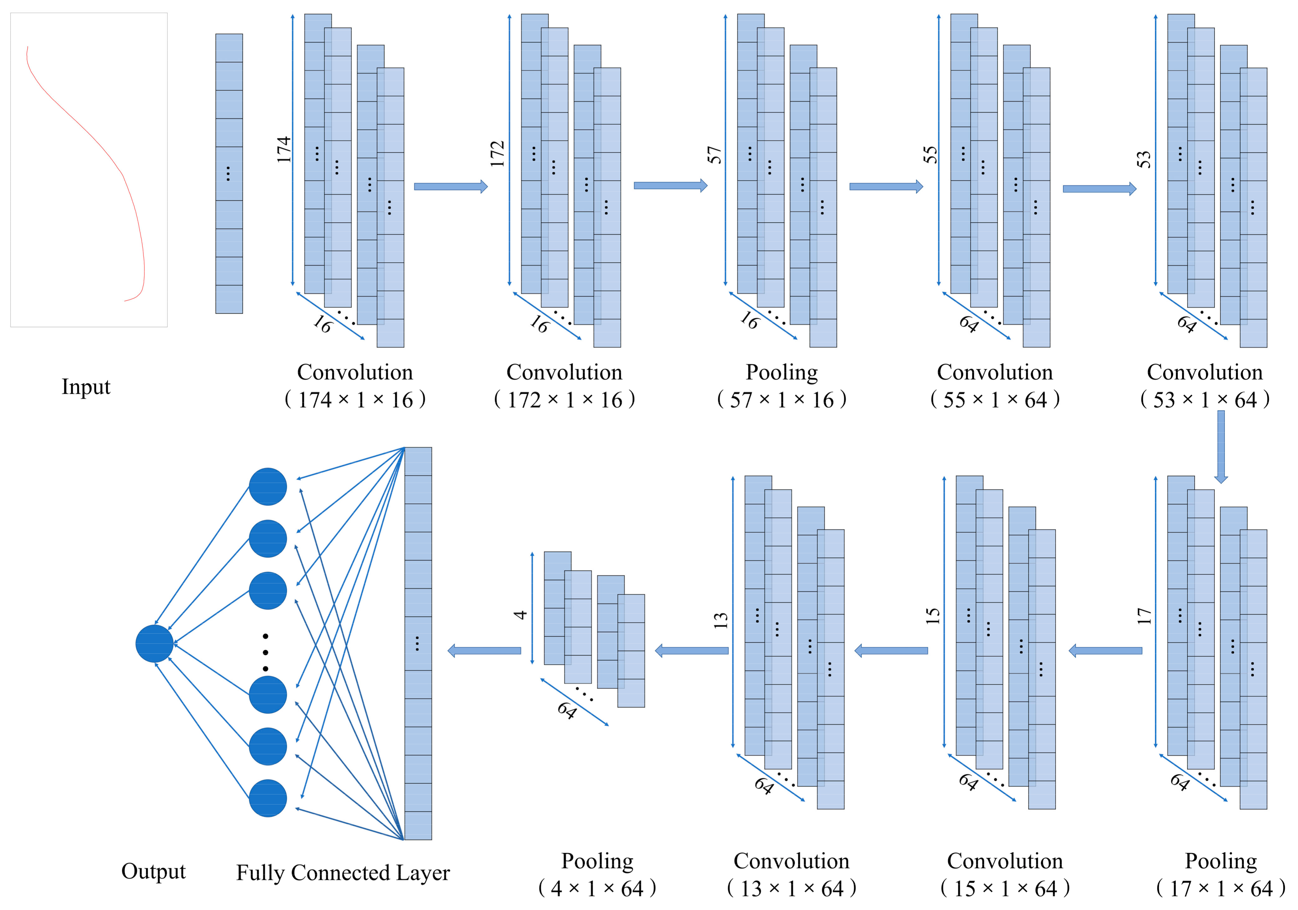
A 1D-CNN architecture was designed for this study. The structure of the 1D-CNN and the flowchart of operation as shown in Figure 2. In detail, 1D-CNN includes 13 layers, including input layer-convolution layer C1 and C2, Pooling layer S3-convolution layer C4 and C5, Pooling layer S6-convolution layer C7 and C8, Pooling layer S9-Fully connected layer F10 and F11, and output. Compared with traditional CNN, a flattened layer was developed in fully connected layer F10 to avoid the multi-dimensional output feature that cannot be directly connected to the full connection layer F11. Table 1 shows the different classification accuracies of 1D-CNN with decreasing layers. It is clear that the 13 layers architecture performed best.
Since the network cannot recognize labels of type 0, 1, and 2, category labels need to be converted into one-hot encoding to store the n-bit state in the form of 0,1 in the n-bit register. Based on the initial size of the input dimension, we used a smaller convolution kernel and a deeper network [50]. Different from traditional CNN, the input of 1D-CNN was one-dimensional, and, accordingly, its convolution layer and pooling layer were also one-dimensional. A one-dimensional convolution layer (Conv1D) with a size of 3 × 1 and a stride size of 1 was used to extract features. A one-dimensional pooling layer with a 3 × 1 kernel size was added after convolution to retain the main features as much as possible. The pooling operation adopted the maximum pooling method. Valid padding was used for convolution and pooling operations. After valid padding, the output size was calculated as below:
The Softmax function was used as the activation function of the full connection layer to judge the sample label by comparing the probability. The Softmax function was used rather than the Euclidean Radial Basis Function adopted in LeNet-5, because Softmax can be well applied to multi-classification problems and has better probability distribution characteristics. A Tanh activation function was chosen instead of Relu because Relu considers eigenvalues less than zero as zero, which will lose some original information of samples and increase the sparsity of the network [51]. A categorical-cross entropy loss function integrated with an adaptive moment estimation (Adam) optimizer was employed to improve training [52]. The parameters alpha, beta_1, beta_2, and epsilon of Adam optimizer were set to 0.001, 0.9, 0.999, and 1 × 10⁻⁸ by default, respectively. Table 2 shows more details.
The performance of classification with different batch sizes are listed in Table 3. Meanwhile, due to the small amount of data in this paper, it was reasonable to set the batch size at 1. Finally, the batch size was set as 1 and epochs was set as 100.
The model was based on the tensorflow-cpu version of keras function, within the Python 3.7 integrated Numpy, Pandas, Pyplot, Sckit-learn.
Supervised Support vector machine (SVM) is a classical learning algorithm in machine learning, which can be well applied to binary or nonlinear classification problems [53]. In nonlinear classification, SVM finds the maximum hyperplane by mapping the samples to a higher dimensional space. The kernel function is the key to higher dimensional mapping. The Radial basis function (RBF) was widely adopted as a kernel function in the spectral analysis [54]. In addition, the RBF has two regularization parameters, i.e., c (the penalty coefficient) and g (the kernel parameter). Further, the selection of appropriate parameter values is essential to the model performance. In former research, the particle swarm optimization (PSO) procedure has been well used in SVM parameter selection [55,56]. In this study, we chose the RBF as kernel function and the PSO to search the optional parameter. The searching range of c and g were set to 2−8 to 28. Both PSO and SVM were implemented using the SVM toolbox written in MATLAB software.
2.4.5. Models Assessment
The prediction performance of the classification model was evaluated based on the information of the confusion matrix, which contains parameters such as true positive (TP, positive chestnuts identified as positive), true negative (TN, negative chestnuts identified as negative), false negative (FN, misclassified positive chestnuts), and false positive (FP, misclassified negative chestnuts) [57].
Generally, models were evaluated by accuracy, which represents the ratio of the number of correctly classified samples in each dataset to the total number of samples. The corresponding calculation formula is as follows:
Sensitivity and specificity were used to evaluate the models for further comparison of classification results [58]. Sensitivity and specificity are calculated as follows:
The Kappa coefficient is generally computed to analyze the agreement in test set [59]. There are four categories about Kappa: simple Kappa, linear weighted Kappa, quadratic weighted Kappa, and weighted Kappa; among them, simple Kappa can be used to measure the classification accuracy as follows:
where Po is accuracy, SRi is the sum of the elements in row i, SCi is the sum of the elements in column i, and AE is the sum of all elements in the confusion matrix. All model evaluation coefficients were carried out in SPSS v21.0 (Statistical Product and Service Solutions, IBM Corporation, Armonk, NY, USA).
3. Results and Discussion
3.1. Overview of the Spectra
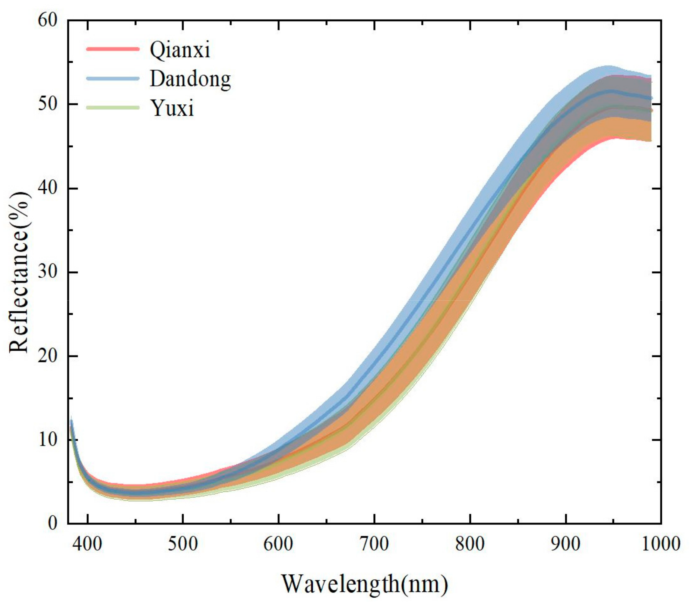
Figure 3 shows the mean spectra with their standard deviations (SDs) from three geographical origins in spectral range of 380–1000 nm. The reflectance in the range of 400–1000 nm is similar with the spectra displayed in Li et al. [60]. In the visible band, the reflectance was affected by red-brown color and chemical composition for chestnuts. In the near-infrared band, the reflectance increased rapidly, which means low absorption and more information. Due to the similar chemical composition, structure, and color presentation, the overall absorption characteristics of chestnuts from different geographical origins were similar. As shown in Figure 3, the spectral regions of the spectra overlapped severely. Thus, it is still difficult to distinguish origins by directly observing the spectra, and further stoichiometric analysis is required.
3.2. PCA Score Plot
Principal component analysis (PCA) is known as an effective unsupervised clustering analysis method. In PCA processing, the maximum variance among samples is set as the objective function, and then the feature vectors representing all the samples will be obtained. After that, the samples will be projected to the new feature vector for the preliminary judgment of origin identification [61]. Figure 4a visualizes the first three PC scores of 417 chestnut clusters into three-dimensional scatter plots. Specifically, the first and second principal components (PC1 and PC2) explain a total of 96% variance of the samples. Although the third principal component (PC3) only explained 3.27%, the addition of PC3 can intuitively see the spatial distribution of samples in three different groups. Samples from three different origins were drawn by three ellipses in different colors to display the distribution more intuitively. As shown in Figure 4a, three ellipses cover different regions, but a large part overlap. More specifically, samples from Qianxi and Yuxi overlapped seriously, and the scattered points of Dandong samples were relatively concentrated, while the samples from Qianxi and Yuxi were relatively scattered. The loading lines of the first two PCs are shown in Figure 4b. The curves in this figure show the contribution of 176 spectral feature points to PC1 and PC2. In the PC2 loading line, 930 nm contributes significantly to PC2 which corresponds to the third overtone of C-H stretching vibration in the aliphatic methylene group [62]. Moreover, the wavelength of 970 nm corresponds to the second overtone of O-H stretching vibration of water [63], but it was influenced by the C-H bonds of lipids at 930 nm [64]. The PC2 curve shows a valley around 720 nm, which corresponds to the fifth overtone of C-H stretching vibration. In conclusion, original spectra have a certain potential in the identification of Chinese chestnut origin. However, further data processing is still needed to improve the accuracy of classification due to the high overlap of spectral regions.
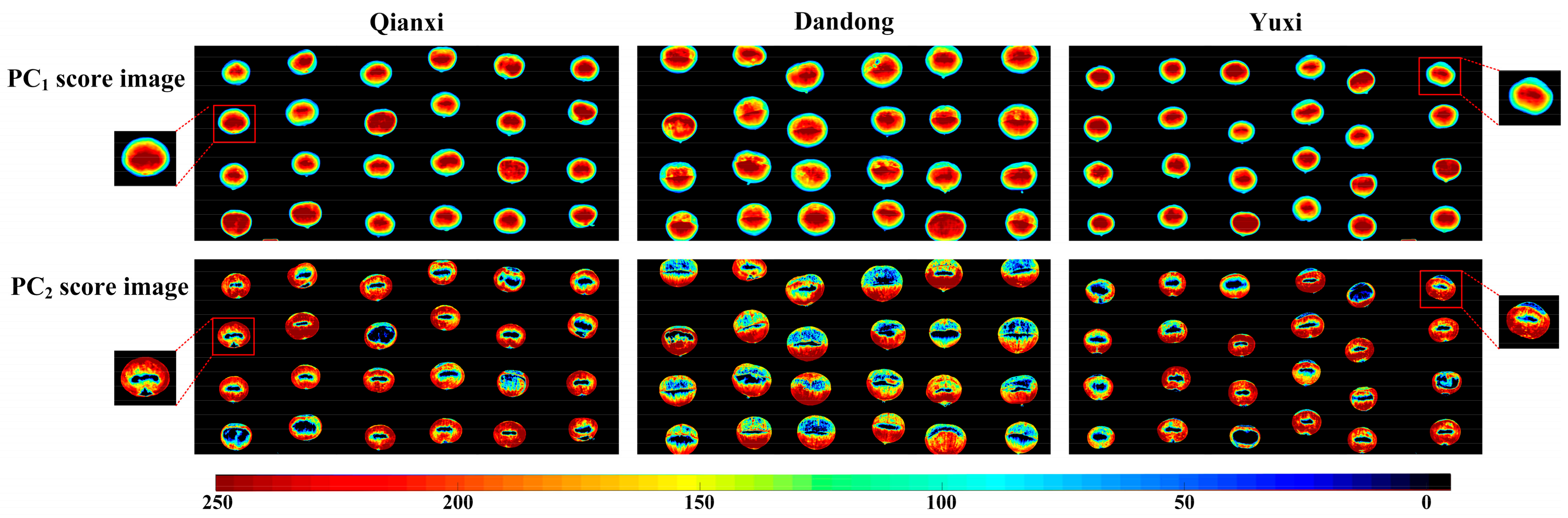
Considering that Figure 3 and Figure 4 were both based on the average spectral mapping of Chinese chestnuts, the spectral information at hyperspectral pixels was not fully utilized. On the contrary, PC score images depict the pixel-wise PC scores [65]. As PC1 and PC2 explain a total of 96% variance, only the first two PC score images were plotted. It can be seen from the color bar in Figure 5 that different PC scores correspond to different colors. All background information was masked in black after PC transformation. It is evident in Figure 5 that the surrounding edge of each chestnut appears blue, and the middle region appears red or orange. This color difference in individual chestnut space can be well explained by the changes of its own shape. However, the PC1 plotting line shows no significant differences among chestnuts from different geographical origins, as with PC2. Thus, further studies are still required to determine the origin accurately.
3.3. Analysis of Classification Model Based on Full Spectra
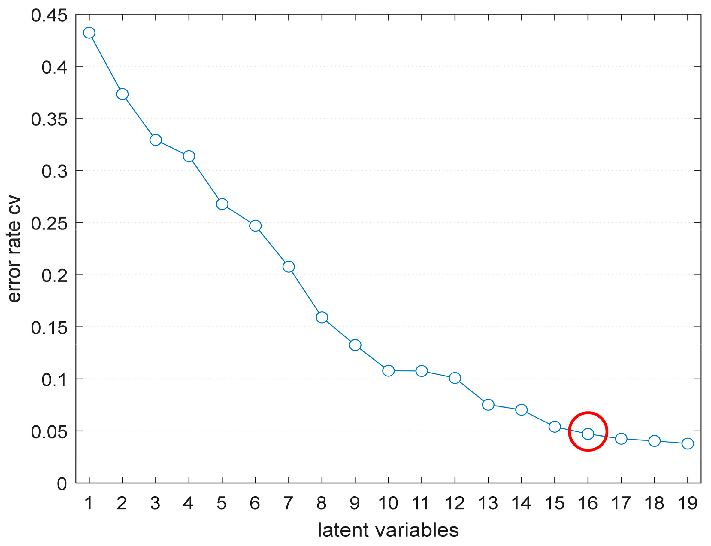
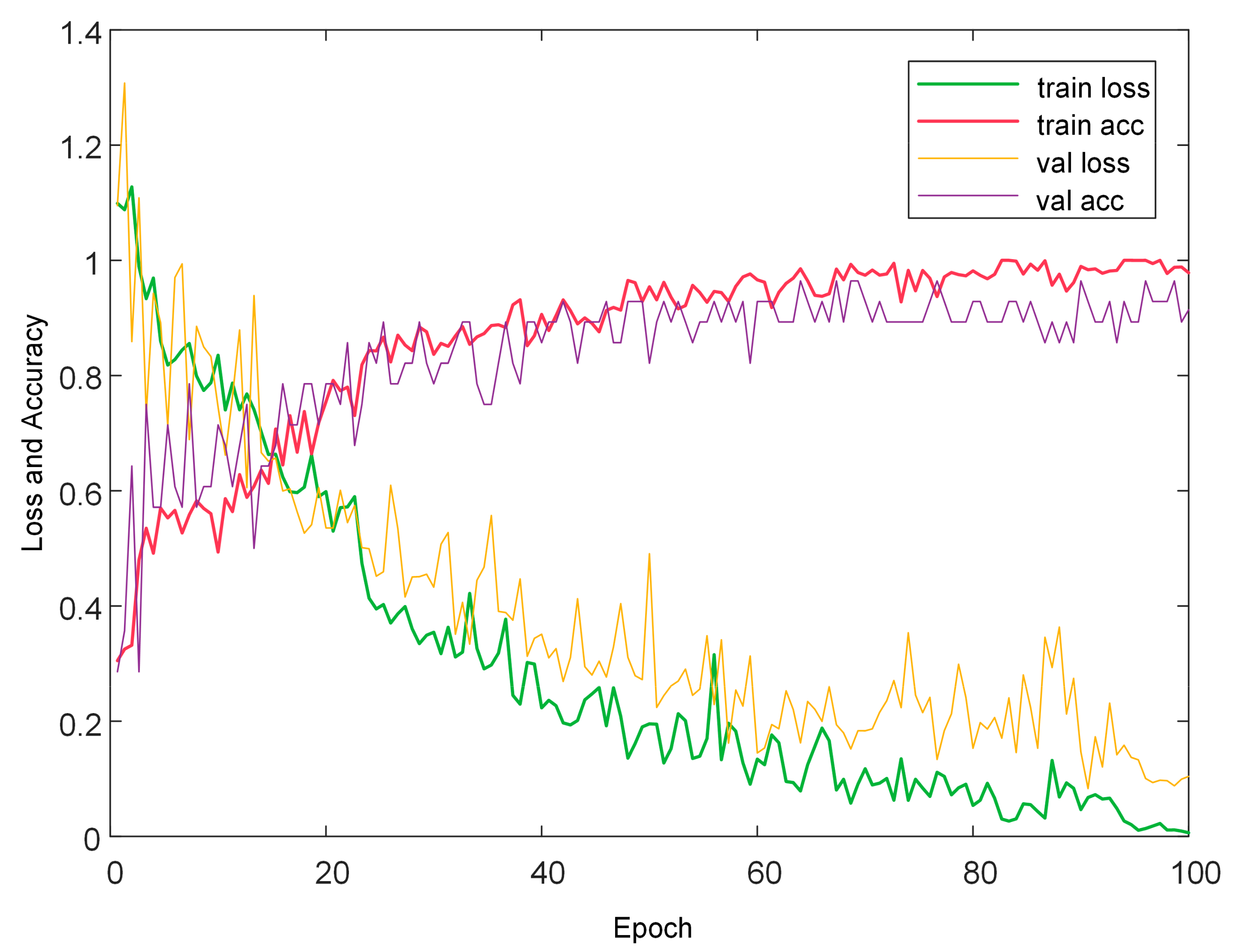
For a more intuitive comparison of different models, the accuracies of PLS-DA, 1D-CNN, and PSO-SVM models with their optimal parameters are listed in Table 4. These models were all built based on full wavelengths (383.4–990.4 nm) with or without preprocessings. The second column in Table 4 shows the preprocessing methods used in modeling, including none, SNV, SNV-detrend, normalization, and first- and second-derivative (SG-1der and SG-2der). The last column in Table 4 shows the optimal parameters of the model. Figure 6 visualizes the process of finding LVs in the PLS-DA model based on raw spectra. After that, the value of LVs was finalized as 16, because the error rate corresponding to the 16 LVs has been around 0.05, and the improvement of accuracy was not obvious since then. Figure 7 visualizes the accuracy and loss curves of 1D-CNN model based on raw spectra. With the increase of epochs, the accuracy of training set and validation set was increasing, while both losses were decreasing. The curve trend of training set and cross-validation set was the same, and with no overfitting.
In the classification models, the classification accuracies of models with preprocessings were generally better than those without preprocessings. The optimal accuracy (97.12%) of PLS-DA model was based on the SNV-preprocessed spectra. The prediction accuracy of 1D-CNN after preprocessing of SNV-detrend also achieved 97.12%, which was the best among 1D-CNN models. Using SNV-detrend and SNV preprocessing, PSO-SVM classification models both gave a predictive accuracy of 95.68%, which was slightly lower than those of the two above-mentioned models. Although the accuracy of prediction sets pre-processed by SNV and SNV-detrend were the same, the accuracies in calibration set and prediction set for SNV-detrend spectra were superior to the former. Finally, the optimal preprocessing methods of the three models were selected for further analysis.
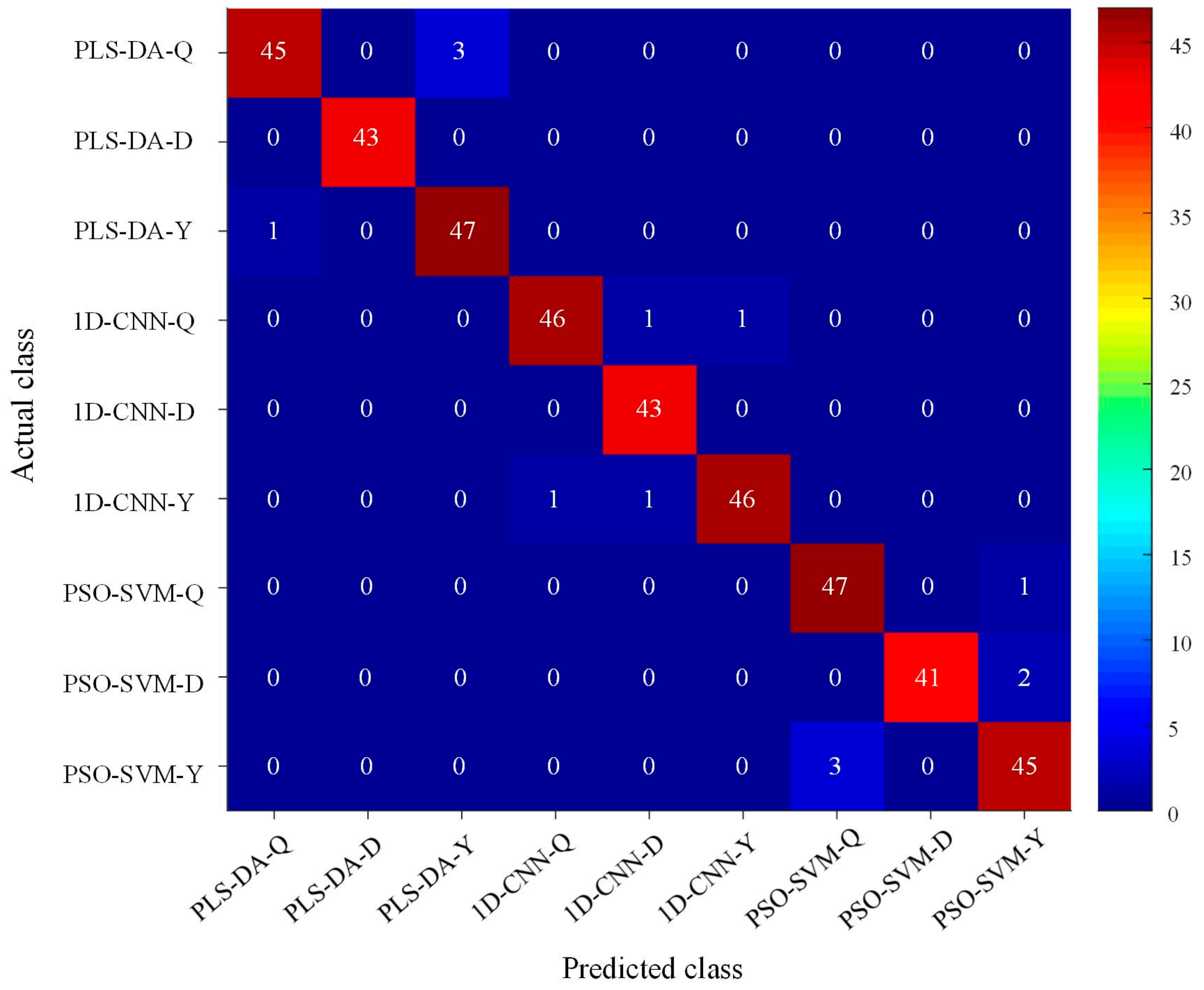
Figure 8 visualizes the result of the PLS-DA, 1D-CNN, PSO-SVM models with optimal spectral preprocessings using confusion matrices. The colors in the confusion matrix were indicated by a heat map with values from 0 to 47. The result indicated that the number of misclassified samples in Dandong group was fewer than in other two groups. In detail, both PLS-DA and CNN models were correct in the prediction of Dandong chestnuts, PSO-SVM misclassified two samples into Yuxi group. For the optimal PLS-DA model, Qianxi chestnuts seemed to be more easily misclassified as Yuxi, three Qianxi chestnuts were classified as Yuxi, and one Yuxi chestnut was misclassified as Qianxi. The optimal 1D-CNN models performed with four misclassifications. In terms of the PSO-SVM models, one Qianxi chestnut and two Dandong chestnuts were misclassified into Yuxi group, and three Yuxi chestnuts were misclassified as Qianxi.
3.4. Characteristic Wavelengths Selection
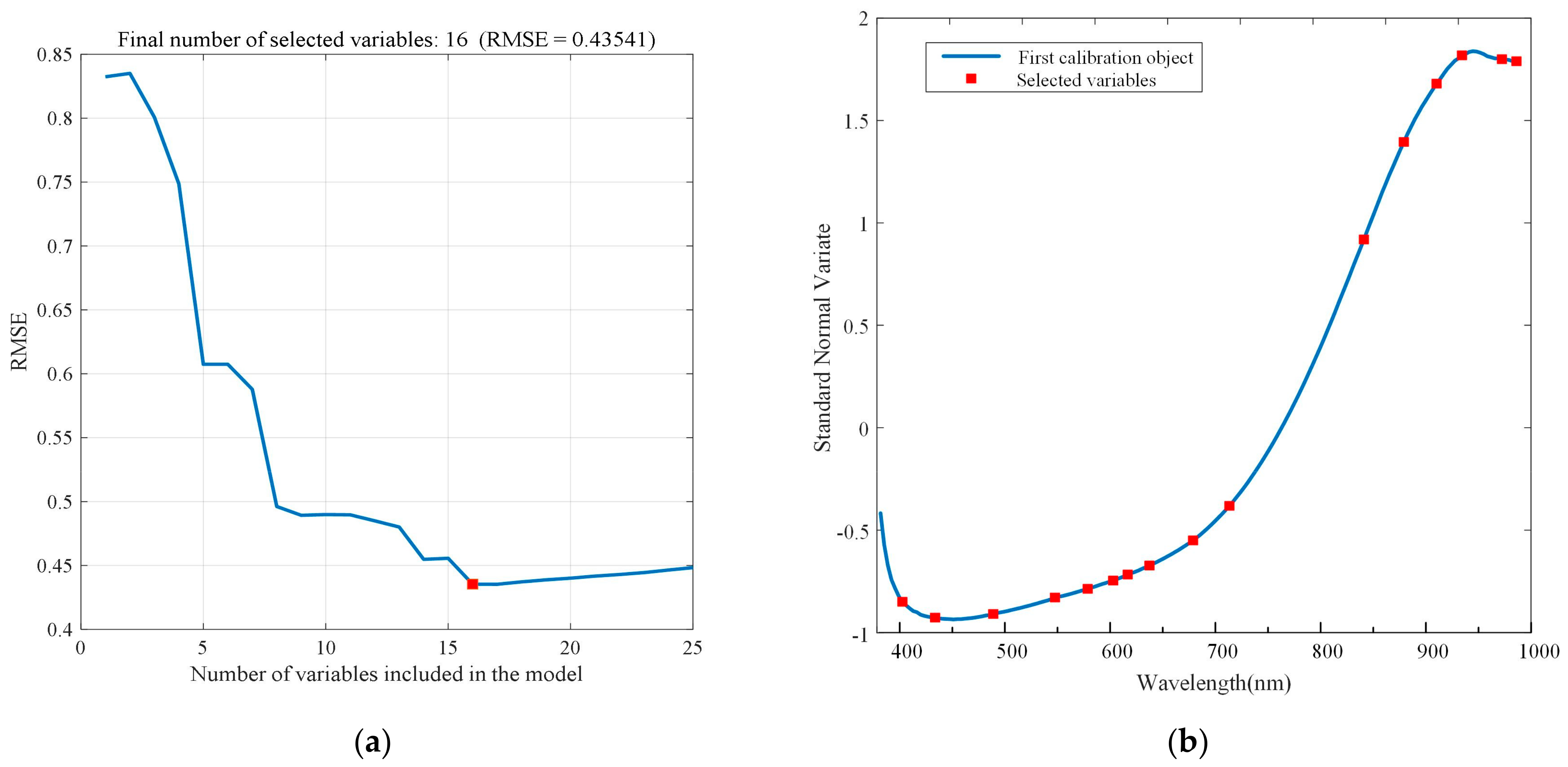
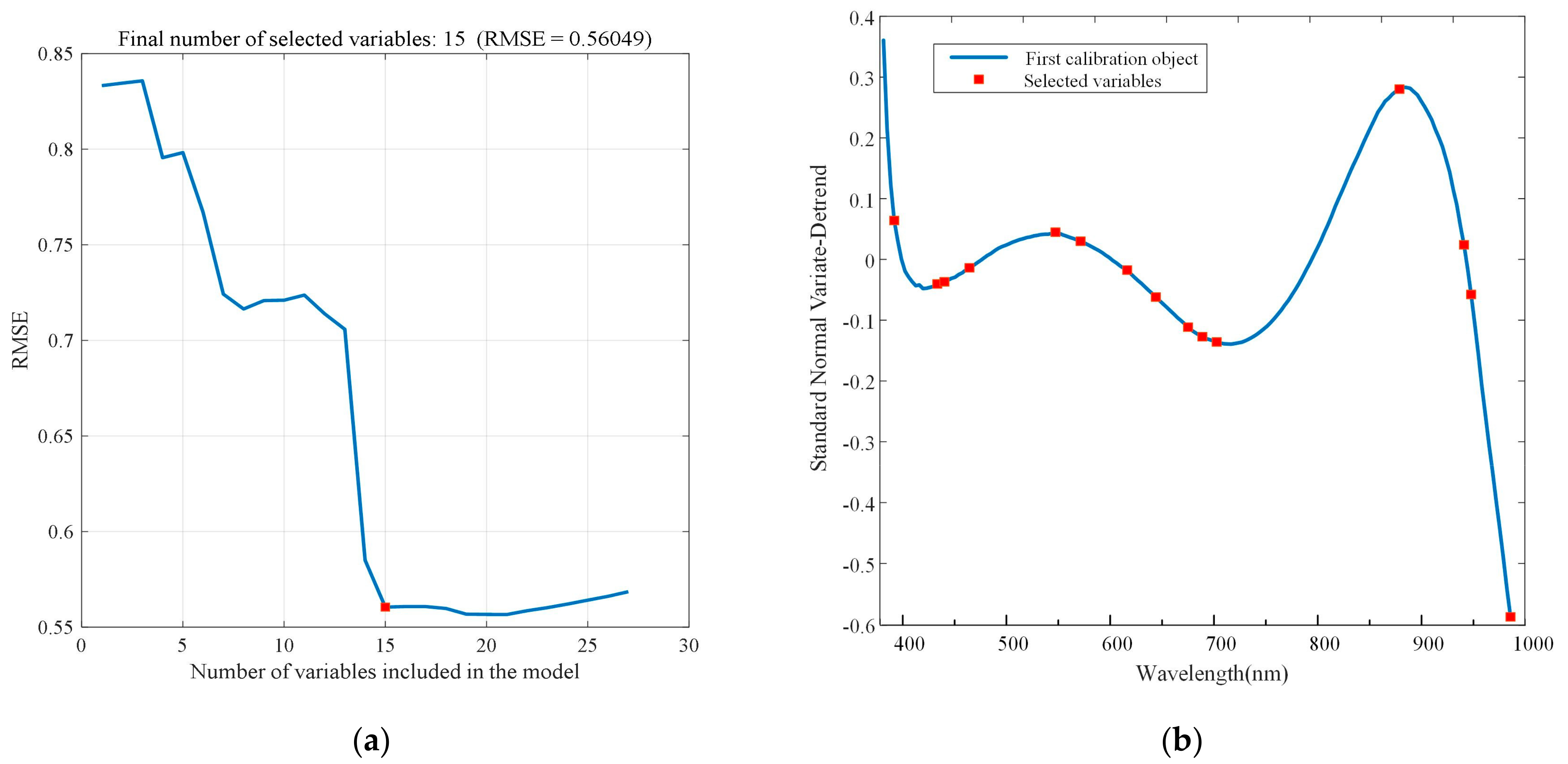
The use of full spectra commonly introduced noise leading to over-fitting, nonlinearities, and loss of efficiency or accuracy. In this study, SPA and CARS algorithms were individually employed to analyze the full spectra (383.4–990.4 nm, 176 bands). Only SNV and SNV-detrend were taken into consideration because these two preprocessings showed good performance as shown in Table 4. The SPA results using SNV preprocessed spectra are shown in Figure 9, and the SPA results after SNV-detrend preprocessing are shown in Figure 10. Before features selection by SPA, the minimum wavelength and maximum wavelength numbers were set as 5 and 30, respectively, according to experience [66].
The RMSE of the ten-fold cross-validation is shown in Figure 9a and Figure 10a. Both figures show a trend of first decreasing and then increasing RMSE value. This trend corresponds to the removal of redundant variables in the early step and the removal of related variables in the later step. In terms of SNV preprocessing, the minimum RMSE was 0.43541, and the number of characteristic wavelengths corresponding to the minimum RMSE was 16. Figure 9b shows the distribution of 16 characteristic wavelength points at full wavelengths; more detailed information of wavelengths are listed in Table 5. For SNV-detrend preprocessing, the RMSE decreased to 0.56049 when the number of characteristic wavelengths reached 15. As a result, Figure 10b shows the distribution of 15 characteristic wavelength points at full wavelengths; more detailed information of wavelengths are listed in Table 5.
In CARS algorithm, Monte Carlo resampling was adopted to select 80% of the subsamples, and 50 Monte Carlo sampling runs were conducted. For the RMSECV, a 10-fold cross-validation was performed. All preceding parameters were chosen empirically [67].
It can be seen from Figure 11a,b that the number of features decreased exponentially with the increasing number of monte Carlo sampling runs. This exhibition was in line with the principle of ‘rough selection first’ and ‘careful selection later’. With the increasing of sampling times, RMSECV descended first and subsequently ascended; this was because CARS eliminated variables with high correlation at the end of steps. The characteristic wavelengths were determined by the lowest RMSECV during sampling runs [68]. As illustrated in Figure 11, the smallest RMSECV corresponds to the blue vertical line. The number of sampling runs based on the smallest RMSECV took place on 28 and 26 respectively. The detailed wavelengths selected by CARS are shown in Table 6.
3.5. Classification Models on Characteristic Wavelengths
After the feature selection steps, the selected wavelengths were imported into traditional machine learning algorithms. As shown in Yang et al. [50], the 1D-CNN model based on full spectra was also listed for easy comparison. More detailed classification results are provided in Table 7.
Overall, the computation time of the two machine learning models were both largely reduced after feature selection. The PLS-DA model decreased from 5.19s of the full spectra to 3.39s based on CARS selection. Although the modeling efficiency in this case was the highest, the results in calibration set and prediction set were the worst among the six models, with accuracy of 95.32% in the calibration set and 93.53% for the prediction set. The selected wavelength greatly reduced the amount of data, which reduced from 176 wavelengths in the full spectra to less than 20, and improved the speed of modeling. In particular, the computation time of PSO-SVM model decreased from 771.01 s in the full spectra to 238.21 s based on CARS-selected wavelengths. In addition, the performance in cross-validation set and prediction set of models developed by CARS-selected wavelengths slightly improved compared with the full spectra, which was the only one of the six models that improved the results. Notably, the PLS-DA and 1D-CNN models revealed the same predictive accuracy of 97.12%.
The evaluation index of the models in Table 7 was the accuracy. However, when the number of various samples was uneven, the accuracy tended to be biased towards the large category (a large number of samples) and abandon the small category (a few numbers of samples). Given the uneven number of predicting samples of different geographical origins, the Kappa coefficient, which can punish the ‘bias’ of the model, was introduced for classification evaluation. To allow further comparison of the specifics of the models, sensitivity and specificity were also presented in Table 8.
As illustrated in Table 8, the Kappa coefficient values of all the models are greater than 0.9; these results can be considered well in classification tasks according to Peng et al. [69]. The Kappa coefficient value of the 1D-CNN model was slightly higher than that of the PLS-DA model. The accuracy of the 1D-CNN model was 97.12% with a sensitivity of 100% for Dandong chestnuts. Meanwhile, the selected PLS-DA model based on SPA showed a perfect classification performance for Qianxi chestnuts, which reached 100%. Taken as a whole, whether it was PLS-DA or CNN model, the chestnut from Qianxi, Dandong, and Yuxi could be well distinguished. These results are encouraging in that they suggest that both SPA-PLS-DA and 1D-CNN models combined with HSI have a great potential for the geographical origin discrimination of Chinese chestnuts.
4. Conclusions
Our study demonstrated that the combination of HSI with chemometrics could be a feasible and effective method for the geographical origin discrimination of Chinese chestnuts. To our knowledge, it is the first study to demonstrate that HSI could well discriminate the geographical origin of Chinese chestnuts. Preprocessing and feature selection steps were carried out to obtain the optimal models of traditional machine learning (PLS-DA, PSO-SVM). Meanwhile, a deep learning method (1D-CNN) based upon preprocessing was given and compared with the optimal model in traditional machine learning.
Our results revealed that the prediction accuracies of developed 1D-CNN and PLS-DA models both achieved 97.12%. Although the Kappa coefficient value of PLS-DA was slightly lower than that of 1D-CNN, the Kappa coefficient values of both models were above 0.95. These results indicated that both the PLS-DA and 1D-CNN models could be well used in origin identification. Considering the HSI also includes image features, future studies will explore if it was possible to further improve the accuracy by adding image features to 2D-CNN. Meanwhile, future studies will include more geographical origins of Chinese chestnuts to improve the generalization ability of the models.
Author Contributions
Conceptualization, X.L.; data curation, X.J.; formal analysis, M.S.; funding acquisition, H.J.; investigation, M.S.; methodology, X.L.; project administration, H.J.; resources, H.J.; software, X.L. and H.J.; supervision, X.J.; validation, X.L., X.J. and H.J.; visualization, H.J.; writing—original draft, X.L. and H.J.; writing—review & editing, X.J. All authors have read and agreed to the published version of the manuscript.
Funding
This work was funded by Jiangsu Agriculture Science and Technology Innovation Fund, grant number CX(20)3040, and the Natural Science Foundation of the Jiangsu Higher Education Institutions of China, grant number 21KJB220013.
Institutional Review Board Statement
Not applicable.
Informed Consent Statement
Not applicable.
Data Availability Statement
The data presented in this study are available on request from the corresponding author.
Acknowledgments
The authors would like to thank the organizations or individuals who have contributed to this manuscript.
Conflicts of Interest
The authors declare no conflict of interest.
References
- Xiao, J.; Gu, C.; Zhu, D.; Wen, X.; Zhou, Q.; Huang, Y. Effects of low relative humidity on respiratory metabolism and energy status revealed new insights on “calcification” in chestnut (Castanea mollissima Bl. cv. ‘Youli’) during postharvest shelf life. Sci. Hortic. 2021, 289, 110473. [Google Scholar] [CrossRef]
- De Vasconcelos, M.C.B.M.; Bennett, R.N.; Rosa, E.A.S.; Ferreira-Cardoso, J.V. Composition of European chestnut (Castanea sativa Mill.) and association with health effects: Fresh and processed products. J. Sci. Food Agric. 2010, 90, 1578–1589. [Google Scholar] [CrossRef] [PubMed]
- Zhou, P.; Zhang, P.; Guo, M.; Li, M.; Wang, L.; Adeel, M.; Shakoor, N.; Rui, Y. Effects of age on mineral elements, amino acids and fatty acids in Chinese chestnut fruits. Eur. Food Res. Technol. 2021, 247, 2079–2086. [Google Scholar] [CrossRef]
- FAO. Food and Agriculture Data. Available online: http://www.fao.org/faostat/zh/#data/QC (accessed on 10 January 2021).
- Han, J.C.; Wang, G.P.; Kong, D.J.; Liu, Q.X.; Zhang, X.Y. Genetic diversity of Chinese chestnut (Castanea mollissima) in Hebei. Acta Hortic. 2007, 760, 573–577. [Google Scholar] [CrossRef]
- Jeon, H.N.; Park, H.W.; Kim, D.-H. Comparative analysis of gallic acid content by chestnut varieties. J. Korea Acad.-Ind. Coop. Soc. 2020, 21, 362–368. [Google Scholar] [CrossRef]
- Krist, S.; Unterweger, H.; Bandion, F.; Buchbauer, G. Volatile compound analysis of SPME headspace and extract samples from roasted Italian chestnuts (Castanea sativa Mill.) using GC-MS. Eur. Food Res. Technol. 2004, 219, 470–473. [Google Scholar] [CrossRef]
- Cirlini, M.; Dall’Asta, C.; Silvanini, A.; Beghe, D.; Fabbri, A.; Galaverna, G.; Ganino, T. Volatile fingerprinting of chestnut flours from traditional Emilia Romagna (Italy) cultivars. Food Chem. 2012, 134, 662–668. [Google Scholar] [CrossRef] [PubMed]
- Park, S.H.; Noh, S.H.; McCarthy, M.J.; Kim, S.M. Internal quality evaluation of chestnut using nuclear magnetic resonance. Int. J. Food Eng. 2021, 17, 57–63. [Google Scholar] [CrossRef]
- Correia, P.; Cruz-Lopes, L.; Beirao-da-Costa, L. Morphology and structure of chestnut starch isolated by alkali and enzymatic methods. Food Hydrocoll. 2012, 28, 313–319. [Google Scholar] [CrossRef]
- Kan, L.; Li, Q.; Xie, S.; Hu, J.; Wu, Y.; Ouyang, J. Effect of thermal processing on the physicochemical properties of chestnut starch and textural profile of chestnut kernel. Carbohydr. Polym. 2016, 151, 614–623. [Google Scholar] [CrossRef]
- Zhang, D.; Feng, X.; Xu, C.; Xia, D.; Liu, S.; Gao, S.; Zheng, F.; Liu, Y. Rapid discrimination of Chinese dry-cured hams based on Tri-step infrared spectroscopy and computer vision technology. Spectrochim. Acta Part A 2020, 228, 117842. [Google Scholar] [CrossRef] [PubMed]
- Srinuttrakul, W.; Mihailova, A.; Islam, M.D.; Liebisch, B.; Maxwell, F.; Kelly, S.D.; Cannavan, A. Geographical differentiation of Hom Mali rice cultivated in different regions of Thailand using FTIR-ATR and NIR spectroscopy. Foods 2021, 10, 1951. [Google Scholar] [CrossRef] [PubMed]
- Marquez, C.; Isabel Lopez, M.; Ruisanchez, I.; Pilar Callao, M. FT-Raman and NIR spectroscopy data fusion strategy for multivariate qualitative analysis of food fraud. Talanta 2016, 161, 80–86. [Google Scholar] [CrossRef] [PubMed]
- Biancolillo, A.; Luca, S.D.; Bassi, S.; Roudier, L.; Marini, F. Authentication of an Italian PDO hazelnut (“Nocciola Romana”) by NIR spectroscopy. Environ. Sci. Pollut. Res. 2018, 25, 1–7. [Google Scholar] [CrossRef] [PubMed]
- Manfredi, M.; Robotti, E.; Quasso, F.; Mazzucco, E.; Marengo, E. Fast classification of hazelnut cultivars through portable infrared spectroscopy and chemometrics. Spectrochim. Acta Part A 2018, 189, 427–435. [Google Scholar] [CrossRef] [PubMed]
- Carvalho, L.C.; Morais, C.L.M.; Lima, K.M.G.; Leite, G.W.P.; Oliveira, G.S.; Casagrande, I.P.; Santos Neto, J.P.; Teixeira, G.H.A. Using intact nuts and near infrared spectroscopy to classify macadamia cultivars. Food Anal. Method. 2018, 11, 1857–1866. [Google Scholar] [CrossRef] [Green Version]
- Arndt, M.; Drees, A.; Ahlers, C.; Fischer, M. Determination of the geographical origin of walnuts (Juglans regia L.) using Near-Infrared spectroscopy and chemometrics. Foods 2020, 9, 1860. [Google Scholar] [CrossRef] [PubMed]
- Nogalesbueno, J.; Feliz, L.; Bacabocanegra, B.; Rato, A.E. Comparative study on the use of three different near infrared spectroscopy recording methodologies for varietal discrimination of walnuts. Talanta 2019, 206, 120189. [Google Scholar] [CrossRef] [PubMed]
- Moscetti, R.; Berhe, D.H.; Agrimi, M.; Haff, R.P.; Liang, P.; Ferri, S.; Monarca, D.; Massantini, R. Pine nut species recognition using NIR spectroscopy and image analysis. J. Food Eng. 2021, 292, 110357. [Google Scholar] [CrossRef]
- Huang, Y.; Si, W.; Chen, K.; Sun, Y. Assessment of tomato maturity in different layers by spatially resolved spectroscopy. Sensors 2020, 20, 7229. [Google Scholar] [CrossRef]
- Ni, C.; Li, Z.Y.; Zhang, X.; Sun, X.Y.; Huang, Y.P.; Zhao, L.; Zhu, T.T.; Wang, D.Y. Online sorting of the film on cotton based on deep learning and hyperspectral imaging. IEEE Access 2020, 8, 93028–93038. [Google Scholar] [CrossRef]
- Huang, Y.P.; Yang, Y.T.; Sun, Y.; Zhou, H.Y.; Chen, K.J. Identification of apple varieties using a multichannel hyperspectral imaging system. Sensors 2020, 20, 5120. [Google Scholar] [CrossRef] [PubMed]
- Qiu, Z.; Chen, J.; Zhao, Y.; Zhu, S.; He, Y.; Zhang, C. Variety identification of single rice seed using hyperspectral imaging combined with convolutional neural network. Appl. Sci. 2018, 8, 212. [Google Scholar] [CrossRef] [Green Version]
- Vresak, M.; Olesen, M.H.; Gislum, R.; Bavec, F.; Jorgensen, J.R. The use of image-spectroscopy technology as a diagnostic method for seed health testing and variety identification. PLoS ONE 2016, 11, e0152011. [Google Scholar] [CrossRef] [PubMed]
- Bao, Y.D.; Mi, C.X.; Wu, N.; Liu, F.; He, Y. Rapid classification of wheat grain varieties using hyperspectral imaging and chemometrics. Appl. Sci. 2019, 9, 4119. [Google Scholar] [CrossRef] [Green Version]
- Kamruzzaman, M.; Barbin, D.; ElMasry, G.; Sun, D.W.; Allen, P. Potential of hyperspectral imaging and pattern recognition for categorization and authentication of red meat. Innov. Food Sci. Emerg. Technol. 2012, 16, 316–325. [Google Scholar] [CrossRef]
- Steinbrener, J.; Posch, K.; Leitner, R. Hyperspectral fruit and vegetable classification using convolutional neural networks. Comput. Electron. Agr. 2019, 162, 364–372. [Google Scholar] [CrossRef]
- Qin, J.W.; Vasefi, F.; Hellberg, R.S.; Akhbardeh, A.; Isaacs, R.B.; Yilmaz, A.G.; Hwang, C.S.; Baek, I.; Schmidt, W.F.; Kim, M.S. Detection of fish fillet substitution and mislabeling using multimode hyperspectral imaging techniques. Food Control 2020, 114, 107234. [Google Scholar] [CrossRef]
- Baek, I.; Kim, M.S.; Cho, B.-K.; Mo, C.; Barnaby, J.Y.; McClung, A.M.; Oh, M. Selection of optimal hyperspectral wavebands for detection of discolored, diseased rice seeds. Appl. Sci. 2019, 9, 1027. [Google Scholar] [CrossRef] [Green Version]
- Mo, C.; Kim, G.; Lim, J.; Kim, M.S.; Cho, H.; Cho, B.-K. Detection of lettuce discoloration using hyperspectral reflectance imaging. Sensors 2015, 15, 29511–29534. [Google Scholar] [CrossRef] [Green Version]
- Xuan, G.; Gao, C.; Shao, Y.; Wang, X.; Wang, Y.; Wang, K. Maturity determination at harvest and spatial assessment of moisture content in okra using Vis-NIR hyperspectral imaging. Postharvest Biol. Technol. 2021, 180, 111597. [Google Scholar] [CrossRef]
- Rajkumar, P.; Wang, N.; Elmasry, G.; Raghavan, G.S.V.; Gariepy, Y. Studies on banana fruit quality and maturity stages using hyperspectral imaging. J. Food Eng. 2012, 108, 194–200. [Google Scholar] [CrossRef]
- Chu, X.; Wang, W.; Ni, X.Z.; Li, C.Y.; Li, Y.F. Classifying maize kernels naturally infected by fungi using near-infrared hyperspectral imaging. Infrared Phys. Technol. 2020, 105, 103242. [Google Scholar] [CrossRef]
- Chen, S.Y.; Chang, C.Y.; Ou, C.S.; Lien, C.T. Detection of insect damage in green coffee beans using VIS-NIR hyperspectral imaging. Remote Sens. 2020, 12, 2348. [Google Scholar] [CrossRef]
- Feng, L.; Zhu, S.S.; Lin, F.C.; Su, Z.Z.; Yuan, K.P.; Zhao, Y.Y.; He, Y.; Zhang, C. Detection of oil chestnuts infected by blue mold using Near-Infrared hyperspectral imaging combined with artificial neural networks. Sensors 2018, 18, 1944. [Google Scholar] [CrossRef] [Green Version]
- Park, S.H.; Lim, K.T.; Lee, H.; Lee, S.H.; Sang, H.N. Prediction of soluble solids content of chestnut using VIS/NIR spectroscopy. J. Biosyst. Eng. 2013, 38, 185–191. [Google Scholar] [CrossRef]
- Liu, Q.; Zhou, D.D.; Tu, S.Y.; Xiao, H.; Zhang, B.; Sun, Y.; Pan, L.Q.; Tu, K. Quantitative visualization of fungal contamination in peach fruit using hyperspectral imaging. Food Anal. Methods 2020, 13, 1262–1270. [Google Scholar] [CrossRef]
- Zhang, J.; Dai, L.M.; Cheng, F. Classification of frozen corn seeds using hyperspectral VIS/NIR reflectance imaging. Molecules 2019, 24, 149. [Google Scholar] [CrossRef] [Green Version]
- Guo, W.C.; Zhao, F.; Dong, J.L. Nondestructive measurement of soluble solids content of kiwifruits using Near-Infrared hyperspectral imaging. Food Anal. Methods 2016, 9, 38–47. [Google Scholar] [CrossRef]
- Amanah, H.Z.; Wakholi, C.; Perez, M.; Faqeerzada, M.A.; Tunny, S.S.; Masithoh, R.E.; Choung, M.G.; Kim, K.H.; Lee, W.H.; Cho, B.K. Near-Infrared Hyperspectral Imaging (NIR-HSI) for nondestructive prediction of anthocyanins content in black rice seeds. Appl. Sci. 2021, 11, 4841. [Google Scholar] [CrossRef]
- Barnes, R.J.; Dhanoa, M.S.; Lister, S.J. Standard normal variate transformation and De-Trending of Near-Infrared diffuse reflectance spectra. Appl. Spectrosc. 2016, 43, 772–777. [Google Scholar] [CrossRef]
- Huang, Z.; Zhu, T.; Li, Z.; Ni, C. Non-destructive testing of moisture and nitrogen content in pinus massoniana seedling leaves with NIRS based on MS-SC-CNN. Appl. Sci. 2021, 11, 2754. [Google Scholar] [CrossRef]
- Xiao, Q.L.; Bai, X.L.; He, Y. Rapid screen of the color and water content of fresh-cut potato tuber slices using hyperspectral imaging coupled with multivariate analysis. Foods 2020, 9, 94. [Google Scholar] [CrossRef] [Green Version]
- Sanchez-Esteva, S.; Knadel, M.; Kucheryavskiy, S.; de Jonge, L.W.; Rubaek, G.H.; Hermansen, C.; Heckrath, G. Combining Laser-Induced breakdown spectroscopy (LIBS) and visible Near-Infrared spectroscopy (Vis-NIRS) for soil phosphorus determination. Sensors 2020, 20, 5419. [Google Scholar] [CrossRef]
- Andersen, A.H.; Rayens, W.S.; Liu, Y.; Smith, C.D. Partial least squares for discrimination. Magn. Reson. Imaging 2012, 30, 446–452. [Google Scholar] [CrossRef] [Green Version]
- Perez, N.F.; Ferre, J.; Boque, R. Calculation of the reliability of classification in discriminant partial least-squares binary classification. Chemom. Intell. Lab. Syst. 2009, 95, 122–128. [Google Scholar] [CrossRef]
- Patel, H.; Upla, K.P. A shallow network for hyperspectral image classification using an autoencoder with convolutional neural network. Multimed. Tools. Appl. 2021, 1–20. [Google Scholar] [CrossRef]
- Sellami, A.; Tabbone, S. Deep neural networks-based relevant latent representation learning for hyperspectral image classification. Pattern Recogn. 2021, 121, 108224. [Google Scholar] [CrossRef]
- Yang, S.; Li, C.; Mei, Y.; Liu, W.; Liu, R.; Chen, W.; Han, D.; Xu, K. Determination of the geographical origin of coffee beans using terahertz spectroscopy combined with machine learning methods. Front. Nutr. 2021, 8, 680627. [Google Scholar] [CrossRef]
- Wang, Q.; Zhao, W.F.; Ren, J.D. Intrusion detection algorithm based on image enhanced convolutional neural network. J. Intell. Fuzzy Syst. 2021, 41, 2183–2194. [Google Scholar] [CrossRef]
- Kingma, D.P.; Ba, J. Adam: A method for stochastic optimization. In Proceedings of the 3rd International Conference for Learning Representations, San Diego, CA, USA, 7–9 May 2015. [Google Scholar]
- Yang, Q.F.; Zhang, H.J.; Xia, J.; Zhang, X.L. Evaluation of magnetic resonance image segmentation in brain low-grade gliomas using support vector machine and convolutional neural network. Quant. Imag. Med. Surg. 2021, 11, 300–316. [Google Scholar] [CrossRef]
- Huang, K.; Wang, H.J.; Xu, H.R.; Wang, J.P.; Ying, Y.B. NIR spectroscopy based on least square support vector machines for quality prediction of tomato juice. Spectrosc. Spect. Anal. 2009, 29, 931–934. [Google Scholar] [CrossRef]
- Li, Y.; Via, B.K.; Young, T.; Li, Y.X. Visible-Near Infrared spectroscopy and chemometric methods for wood density prediction and origin/species identification. Forests 2019, 10, 1078. [Google Scholar] [CrossRef] [Green Version]
- Li, X.X.; Bi, S.H.; Zhang, Y.H.; Shen, T.; IEEE. SVM-based apple classification of soluble solids content by Near-infrared spectroscopy. In Proceedings of the 31st Chinese Control and Decision Conference (CCDC), Nanchang, China, 3–5 June 2019; pp. 4001–4005. [Google Scholar]
- Kurosaki, K.; Wu, R.; Uesawa, Y. A toxicity prediction tool for potential agonist/antagonist activities in molecular initiating events based on chemical structures. Int. J. Mol. Sci. 2020, 21, 7853. [Google Scholar] [CrossRef]
- Doheny, E.P.; Walsh, C.; Foran, T.; Greene, B.R.; Fan, C.W.; Cunningham, C.; Kenny, R.A. Falls classification using tri-axial accelerometers during the five-times-sit-to-stand test. Gait Posture 2013, 38, 1021–1025. [Google Scholar] [CrossRef]
- Duan, G.H.; Zhang, J.C.; Zhang, S.P. Assessment of landslide susceptibility based on multiresolution image segmentation and geological factor ratings. Int. J. Environ. Res. Public Health 2020, 17, 7863. [Google Scholar] [CrossRef] [PubMed]
- Li, B.C.; Hou, B.L.; Zhou, Y.; Zhao, M.T.; Zhang, D.W.; Hong, R.J. Detection of waxed chestnuts using visible and Near-Infrared hyper-spectral imaging. Food Sci. Technol. Res. 2016, 22, 267–277. [Google Scholar] [CrossRef] [Green Version]
- Imbao, J.; van Bokhoven, J.A.; Clark, A.; Nachtegaal, M. Elucidating the mechanism of heterogeneous Wacker oxidation over Pd-Cu/zeolite Y by transient XAS. Nat. Commun. 2020, 11, 1118. [Google Scholar] [CrossRef] [Green Version]
- Wu, D.; Sun, D.W. Application of visible and near infrared hyperspectral imaging for non-invasively measuring distribution of water-holding capacity in salmon flesh. Talanta 2013, 116, 266–276. [Google Scholar] [CrossRef]
- Bobelyn, E.; Serban, A.S.; Nicu, M.; Lammertyn, J.; Nicolai, B.M.; Saeys, W. Postharvest quality of apple predicted by NIR-spectroscopy: Study of the effect of biological variability on spectra and model performance. Postharvest Biol. Technol. 2010, 55, 133–143. [Google Scholar] [CrossRef]
- Kukreti, S.; Cerussi, A.; Tromberg, B.; Gratton, E. Intrinsic tumor biomarkers revealed by novel double-differential spectroscopic analysis of near-infrared spectra. J. Biomed. Opt. 2007, 12, 020509. [Google Scholar] [CrossRef]
- Feng, L.; Zhu, S.S.; Zhang, C.; Bao, Y.D.; Gao, P.; He, Y. Variety identification of raisins using Near-Infrared hyperspectral imaging. Molecules 2018, 23, 2907. [Google Scholar] [CrossRef] [PubMed] [Green Version]
- Wu, X.; Song, X.L.; Qiu, Z.J.; He, Y. Mapping of TBARS distribution in frozen-thawed pork using NIR hyperspectral imaging. Meat Sci. 2016, 113, 92–96. [Google Scholar] [CrossRef]
- Wang, Y.J.; Li, T.H.; Li, L.Q.; Ning, J.M.; Zhang, Z.Z. Evaluating taste-related attributes of black tea by micro-NIRS. J. Food Eng. 2021, 290, 110181. [Google Scholar] [CrossRef]
- Su, W.H.; Yang, C.; Dong, Y.; Johnson, R.; Steffenson, B.J. Hyperspectral imaging and improved feature variable selection for automated determination of deoxynivalenol in various genetic lines of barley kernels for resistance screening. Food Chem. 2021, 343, 128507. [Google Scholar] [CrossRef]
- Peng, X.X.; Wu, W.Y.; Zheng, Y.Y.; Sun, J.Y.; Hu, T.G.; Wang, P. Correlation analysis of land surface temperature and topographic elements in Hangzhou, China. Sci. Rep. 2020, 10, 10451. [Google Scholar] [CrossRef] [PubMed]
Figure 1.
The extraction process of ROI.

Figure 2.
Flow chart of 1D-CNN.

Figure 3.
Average reflectance spectra with standard deviation (SD) of three different origins of chestnuts.
Figure 3.
Average reflectance spectra with standard deviation (SD) of three different origins of chestnuts.

Figure 4.
Spectral PCA for Chinese chestnuts with different varieties. (a) The first three PC score plots, and (b) the first two PC loading lines. PCA, principal component analysis, and PC, principal component.
Figure 4.
Spectral PCA for Chinese chestnuts with different varieties. (a) The first three PC score plots, and (b) the first two PC loading lines. PCA, principal component analysis, and PC, principal component.

Figure 5.
The PC1 and PC2 score images. PC1, first principal component, and PC2, second principal component.
Figure 5.
The PC1 and PC2 score images. PC1, first principal component, and PC2, second principal component.

Figure 6.
The optimal number of LVs determination in the PLS-DA model. LVs: latent variables.

Figure 7.
The accuracy and loss curves of 1D-CNN model without preprocessing.

Figure 8.
Visualized confusion matrix of three different modeling methods based on their optimal preprocessings, where Q, D, and Y represent “Qianxi”, “Dandong”, and “Yuxi”, respectively.
Figure 8.
Visualized confusion matrix of three different modeling methods based on their optimal preprocessings, where Q, D, and Y represent “Qianxi”, “Dandong”, and “Yuxi”, respectively.

Figure 9.
Selection of characteristic wavelengths using SPA after SNV preprocessing: (a) number of effective variables and (b) visualized characteristic wavelengths in the raw spectra.
Figure 9.
Selection of characteristic wavelengths using SPA after SNV preprocessing: (a) number of effective variables and (b) visualized characteristic wavelengths in the raw spectra.

Figure 10.
Selection of characteristic wavelengths using SPA after SNV-detrend preprocessing: (a) number of effective variables and (b) visualized characteristic wavelengths in the raw spectra.
Figure 10.
Selection of characteristic wavelengths using SPA after SNV-detrend preprocessing: (a) number of effective variables and (b) visualized characteristic wavelengths in the raw spectra.

Figure 11.
CARS Running results. (a) CARS wavelength selection after SNV preprocessing and (b) CARS wavelength selection after SNV-detrend preprocessing.
Figure 11.
CARS Running results. (a) CARS wavelength selection after SNV preprocessing and (b) CARS wavelength selection after SNV-detrend preprocessing.


Table 1.
The classification accuracies of 1D-CNN with different layers.
| Deleted Layer | Accuracy (%) | ||
|---|---|---|---|
| Calibration Set | Cross-Validation Set | Prediction Set | |
| None | 97.84 | 91.38 | 92.81 |
| C7, C8, S9 | 94.96 | 92.12 | 89.92 |
| C4, C5, S6, C7, C8, S9 | 64.03 | 60.48 | 56.83 |
Table 2.
Detailed parameters of each layer.
| Layer | Type | Feature Map | Kernel Size | Stride | Padding | Size | Activation Function |
|---|---|---|---|---|---|---|---|
| In | Input | 1 | … | … | … | 176 × 1 × 1 | … |
| Conv1 | Convolution | 16 | 3 × 1 | 1 | 0 | 174 × 1 × 16 | … |
| Conv2 | Convolution | 16 | 3 × 1 | 1 | 0 | 172 × 1 × 16 | tanh |
| S3 | Max pooling | 16 | 3 × 1 | 1 | 0 | 57 × 1 × 16 | … |
| Conv 4 | Convolution | 64 | 3 × 1 | 1 | 0 | 55 × 1 × 64 | … |
| Conv 5 | Convolution | 64 | 3 × 1 | 1 | 0 | 53 × 1 × 64 | tanh |
| S6 | Max pooling | 64 | 3 × 1 | 1 | 0 | 17 × 1 × 64 | … |
| Conv 7 | Convolution | 64 | 3 × 1 | 1 | 0 | 15 × 1 × 64 | … |
| Conv 8 | Convolution | 64 | 3 × 1 | 1 | 0 | 13 × 1 × 64 | tanh |
| S9 | Max pooling | 64 | 3 × 1 | 1 | 0 | 4 × 1 × 64 | … |
| FC10 | Flatten | … | … | … | … | 256 × 1 | … |
| FC11 | Fully connected | … | … | … | … | 3 × 1 | softmax |
| Out | Output | … | … | … | … | 3 × 1 | … |
Table 3.
The classification accuracies of 1D-CNN with different batch sizes.
| Batch Size | Accuracy (%) | ||
|---|---|---|---|
| Calibration Set | Cross-Validation Set | Prediction Set | |
| 1 | 97.84 | 91.38 | 92.81 |
| 8 | 95.68 | 91.04 | 89.93 |
| 16 | 99.64 | 86.63 | 88.49 |
| 32 | 92.81 | 82.76 | 82.73 |
Table 4.
Performance of the classification models based on full wavelengths with or without preprocessings.
Table 4.
Performance of the classification models based on full wavelengths with or without preprocessings.
| Modeling Methods | Preprocessings | Accuracy (%) | Parameters | ||
|---|---|---|---|---|---|
| Calibration Set | Cross-Validation Set | Prediction Set | |||
| PLS-DA | None | 97.84 | 94.96 | 95.68 | LVs = 16 |
| SNV | 99.28 | 98.20 | 97.12 | LVs = 18 | |
| SNV-detrend | 97.84 | 96.04 | 94.96 | LVs = 14 | |
| Normalization | 97.48 | 95.32 | 94.96 | LVs = 15 | |
| SG-1der | 98.56 | 95.32 | 94.96 | LVs = 16 | |
| SG-2der | 100 | 84.89 | 84.17 | LVs = 19 | |
| 1D-CNN | None | 97.84 | 91.38 | 92.81 | / |
| SNV | 97.12 | 83.52 | 95.68 | / | |
| SNV-detrend | 99.64 | 93.13 | 97.12 | / | |
| Normalization | 98.56 | 82.42 | 91.37 | / | |
| SG-1der | 96.40 | 92.49 | 88.49 | / | |
| SG-2der | 100 | 75.61 | 93.53 | / | |
| PSO-SVM | None | 98.20 | 84.17 | 89.93 | / |
| SNV | 96.04 | 91.73 | 95.68 | / | |
| SNV-detrend | 97.84 | 92.81 | 95.68 | / | |
| Normalization | 97.12 | 84.17 | 92.09 | / | |
| SG-1der | 80.22 | 77.70 | 79.86 | / | |
| SG-2der | 73.38 | 66.91 | 71.22 | / | |
Table 5.
The characteristic wavelengths selected by SPA.
| Preprocessings | Number | Selected Wavelengths (nm) |
|---|---|---|
| SNV | 16 | 402.5, 431.5, 483.7, 540, 570.2, 593.9, 607.5, 628, 669.3, 704.1, 835.7, 875.7, 908.6, 934.5, 975.4, 990.4 |
| SNV-detrend | 15 | 392.9, 431.5, 438, 460.8, 540, 563.5, 607.5, 634.8, 665.8, 679.7, 693.6, 875.7, 941.9, 949.3, 990.4 |
Table 6.
The characteristic wavelengths selected by CARS.
| Preprocessings | Number | Selected Wavelengths (nm) |
|---|---|---|
| SNV | 15 | 460.8, 473.8, 523.4, 526.7, 530, 533.3, 536.7, 546.7, 570.2, 573.6, 577, 583.7, 669.3, 686.7, 697.1 |
| SNV-detrend | 18 | 421.8, 460.8, 467.3, 473.8, 523.4, 526.7, 530, 533.3, 570.2, 573.6, 577, 669.3, 686.7, 756.9, 908.6, 912.3, 945.6, 971.7 |
Table 7.
Comparison of performance obtained with machine learning methods based on feature selection.
Table 7.
Comparison of performance obtained with machine learning methods based on feature selection.
| Modeling Methods | Feature Selection | Number | LVs | Accuracy (%) | Computing Time (s) | ||
|---|---|---|---|---|---|---|---|
| Calibration | Cross-Validation | Prediction | |||||
| PLS-DA | FULL | 176 | 18 | 99.28 | 98.2 | 97.12 | 5.19 |
| SPA | 16 | 13 | 98.2 | 97.84 | 97.12 | 3.51 | |
| CARS | 15 | 10 | 95.32 | 93.88 | 93.53 | 3.39 | |
| PSO-SVM | FULL | 176 | \ | 97.84 | 92.81 | 95.68 | 771.01 |
| SPA | 15 | \ | 96.76 | 91.37 | 95.68 | 349.42 | |
| CARS | 18 | \ | 96.76 | 94.24 | 96.4 | 238.21 | |
| 1D-CNN | FULL | 176 | \ | 99.64 | 93.13 | 97.12 | 35.32 |
Table 8.
Confusion matrix of the three sets predicted by SPA-PLS-DA and 1D-CNN models.
| Actual Class | Predicted Class | |||||
|---|---|---|---|---|---|---|
| SPA-PLS-DA | 1D-CNN | |||||
| Qianxi | Dandong | Yuxi | Qianxi | Dandong | Yuxi | |
| Qianxi | 48 | 0 | 0 | 46 | 1 | 1 |
| Dandong | 0 | 42 | 1 | 0 | 43 | 0 |
| Yuxi | 2 | 1 | 45 | 1 | 1 | 46 |
| Sen a (%) | 100 | 97.67 | 93.75 | 95.83 | 100 | 95.83 |
| Spe b (%) | 97.80 | 98.96 | 98.90 | 98.90 | 97.92 | 98.90 |
| Kappa | 0.95677 | 0.95681 | ||||
| Acc c (%) | 97.12 | 97.12 | ||||
a The sensitivity of models; b the specificity of models; and c the prediction accuracy of models.
Publisher’s Note: MDPI stays neutral with regard to jurisdictional claims in published maps and institutional affiliations. |
© 2021 by the authors. Licensee MDPI, Basel, Switzerland. This article is an open access article distributed under the terms and conditions of the Creative Commons Attribution (CC BY) license (https://creativecommons.org/licenses/by/4.0/).
Share and Cite
MDPI and ACS Style
Li, X.; Jiang, H.; Jiang, X.; Shi, M. Identification of Geographical Origin of Chinese Chestnuts Using Hyperspectral Imaging with 1D-CNN Algorithm. Agriculture 2021, 11, 1274. https://0-doi-org.brum.beds.ac.uk/10.3390/agriculture11121274
AMA Style
Li X, Jiang H, Jiang X, Shi M. Identification of Geographical Origin of Chinese Chestnuts Using Hyperspectral Imaging with 1D-CNN Algorithm. Agriculture. 2021; 11(12):1274. https://0-doi-org.brum.beds.ac.uk/10.3390/agriculture11121274
Chicago/Turabian StyleLi, Xingpeng, Hongzhe Jiang, Xuesong Jiang, and Minghong Shi. 2021. "Identification of Geographical Origin of Chinese Chestnuts Using Hyperspectral Imaging with 1D-CNN Algorithm" Agriculture 11, no. 12: 1274. https://0-doi-org.brum.beds.ac.uk/10.3390/agriculture11121274
Note that from the first issue of 2016, this journal uses article numbers instead of page numbers. See further details here.