
Modeling Profitability in the Jamaican Coffee Industry


1
Department of Geography, University of North Alabama, Florence, AL 35632, USA
2
Department of Geography and Anthropology, California State Polytechnic University, Pomona, CA 91768, USA
*
Author to whom correspondence should be addressed.
Agriculture 2021, 11(2), 121; https://0-doi-org.brum.beds.ac.uk/10.3390/agriculture11020121
Submission received: 22 December 2020
/
Revised: 20 January 2021
/
Accepted: 21 January 2021
/
Published: 3 February 2021
(This article belongs to the Special Issue Agricultural Food Marketing, Economics and Policies)
Abstract
:It is well known that producers of agricultural products do not able to capture most of the value from what they grow. As such, it is important for producers to be attuned to the various factors that impact the viability of their products. One such potential avenue for coffee producers is developing a strong awareness of profitability across their respective geographic regions. This research presents a fine-scale geospatial profitability model for coffee production using the test case of the Jamaican Coffee Industry, a sector which once guaranteed profitability but now presents variable (often losing) returns for many producers, this research presents a cost-surface model for coffee production in the island of Jamaica. Results indicated large scale profitability in the 2016–2017 coffee year but limited profitability in the 2019–2019 coffee year, highlighting the important role of revenue fluctuation in island-wide profitability. Results underscore importance of scenario planning in the coffee production cycle. By understanding the spatial properties of profitability producers will obtain better decision-making insight for production and management decisions in the coffee industry around the world. The geospatial profitability model establishes a baseline approach that can be accessed by industry stakeholders of varying technological capacities.
1. Introduction
Coffee is one of the most popular beverages in the world and its economic influence is as big as its popularity. This commodity is the second most valuable good legally traded and over 100 million people derive their livelihood in one way or another from coffee [1,2]. Prices can range from a bargain US$6/lb. for low quality Robusta coffee (Coffea canephora) coffee blends such as Maxwell House or Folgers in a typical U.S. supermarket to over US$100/lb. for high end, single-origin premium Arabica coffee (Coffea arabica) coffees such as Kopi Luwak from Indonesia or the Hacienda La Esmeralda from Panama. However, the prices paid by consumers are not always an indication of the prices received by growers. Moreover, retail prices do not necessarily reflect profitability in coffee production.
The modern development of the global agricultural commodity value chain has shifted value away from the farm and toward the retailer. Researchers have found agricultural producers capture only a small fraction of the overall economic value generated by the global value chain; with small landholders netting even less of the economic benefit. Alternatives to improve farmers’ revenue include increased involvement in vertical integration up the value chain or engaging in cooperative approaches to production [3,4,5,6,7].
In addition to this, fluctuating supply and demand for coffee and steadily rising production costs of inputs regardless of demand further complicate the lives of coffee farmers around the world. According to the International Coffee Organization (ICO), global coffee prices remain the lowest of recent coffee years. This is primarily due to supply exceeding demand—even as global consumption increases; production levels continue to oversupply the market [8,9]. With the realization that producers often realize small profit margins or even losses, the ICO approved a resolution in 2018 to address these issues [8]. Resolution 465 recognizes the impacts of low coffee prices on the livelihoods of coffee farmers including increasing food insecurity, reducing access to health and education, and even cultivation of illicit crops. Therefore, the resolution mandates action in the form of assisting exporting countries to increase their own consumption levels and the strengthening of ties with the international (coffee) roasting industry.
Along with action taken at the (inter)national level, a key avenue for maintaining viability at the local level is for stakeholders in the coffee industry to have a strong awareness of profitability across their respective geographic regions. Stakeholders in the agricultural sector are regularly confronted with challenges which might drive land use change and ultimately agricultural profitability to a substantial degree. The challenges include questions around climate variability, demographic changes, use of land for alternative production (i.e., biofuel production) and ensuring an increase in food production. As profitability drives many agri-business decisions, knowledge about the existing socio-economic landscape, the economic profile of agricultural production, as well as potential impacts on profits provides useful contextual information when agricultural policies are designed [10].
Farmers’ awareness of their geographical, socio-economic region, and profitability may stimulate differentiation of coffee. An increasing number of coffee producers have turned to producing some variety of specialty coffee [11] with the aim of offsetting rising production costs and escaping a stagnant conventional coffee market by selling to a higher income market. For the purposes of this paper, we define coffee producers as those directly involved in the planting, cultivation and harvesting of coffee. They will also be referred to as ‘farmers’ throughout this paper. Consequently, there has been an increasing number of brands competing for a relatively small pool of consumers willing to pay top dollar for their coffee. These coffee marques are spatially scattered around the world and include famous names such as Ethiopia’s Yirgacheffe, Panama’s Hacienda La Esmeralda, Hawaii’s Kona, and Jamaica’s Blue Mountain coffees. Notably, these are exporting regions. They are often characterized by distinctive flavor profiles, small production quantities, and restricted geographic regions. However, even specialty coffee producing region are considered price takers from the international market.
The goal of this research is to present a geospatial profitability model for coffee production at local-level. With increasing competition in this agricultural segment, it has become paramount that coffee stakeholders adopt a more precise approach not just to cultivation but awareness of profitability across their respective production regions. ‘Coffee stakeholders’ refer to all parties involved in the coffee value chain. This includes producers, processors (takes the harvested coffee cherries and prepares it to green bean coffee), roasters (roasts green bean coffee for sale to consumers, retailers or wholesalers), exporters/importers (exports or imports green bean or roasted coffee), retailers/wholesalers (focused on sale of prepared coffee products to consumer/coffee beans intended for retail sale) and public (government) bodies involved in the regulation and sale of coffee.
Incorporating geospatial technologies provides an opportunity for producers to understand the potential for profit at multiple geographic scales—from the sub-acre local (or small) farm level up to the national level. We tested our profitability model using cost and revenue data for the Jamaican coffee industry, a sector which once guaranteed profitability but now presents a great variability on the returns for many producers. In the Jamaican coffee industry, small farmers are the main producers of coffee berries. The information generated by this geospatial profitability model can provide farmers and policymakers better decision-making insight in the year-to-year feasibility and market potential for growing coffee across the island. Given the upcoming challenges of climatic change, market competition and their associated uncertainties, it is important to ensure that such maps of agricultural profit can be reproduced in various scenarios and simulation settings which can allow exploring uncertainties around the impacts on agricultural profits as well.
The result of this research has implications for production and management decisions in the coffee industry around the world. Small farmers who do not have the luxury of large economies of scale can use the results of this research to be ‘nimbler’ and make informed decisions more readily by examining the potential profitability of their lands. This research also highlights the contribution of exogenous factors such as farmgate prices vs. endogenous factors such as land suitability and production methods to farm profitability, even in an agricultural commodity that commands a significantly higher market price. Finally, the model discussed here is designed in such a way to facilitate a ‘plug and play’ functionality to predict potential profitability. Not only does this make it more accessible to stakeholders with variable technological capacities, but it provides an avenue for modification and use on various geospatial software platforms—a real benefit for entities with limited access to or funding for more expensive geospatial software.
2. Materials and Methods
2.1. Study Area
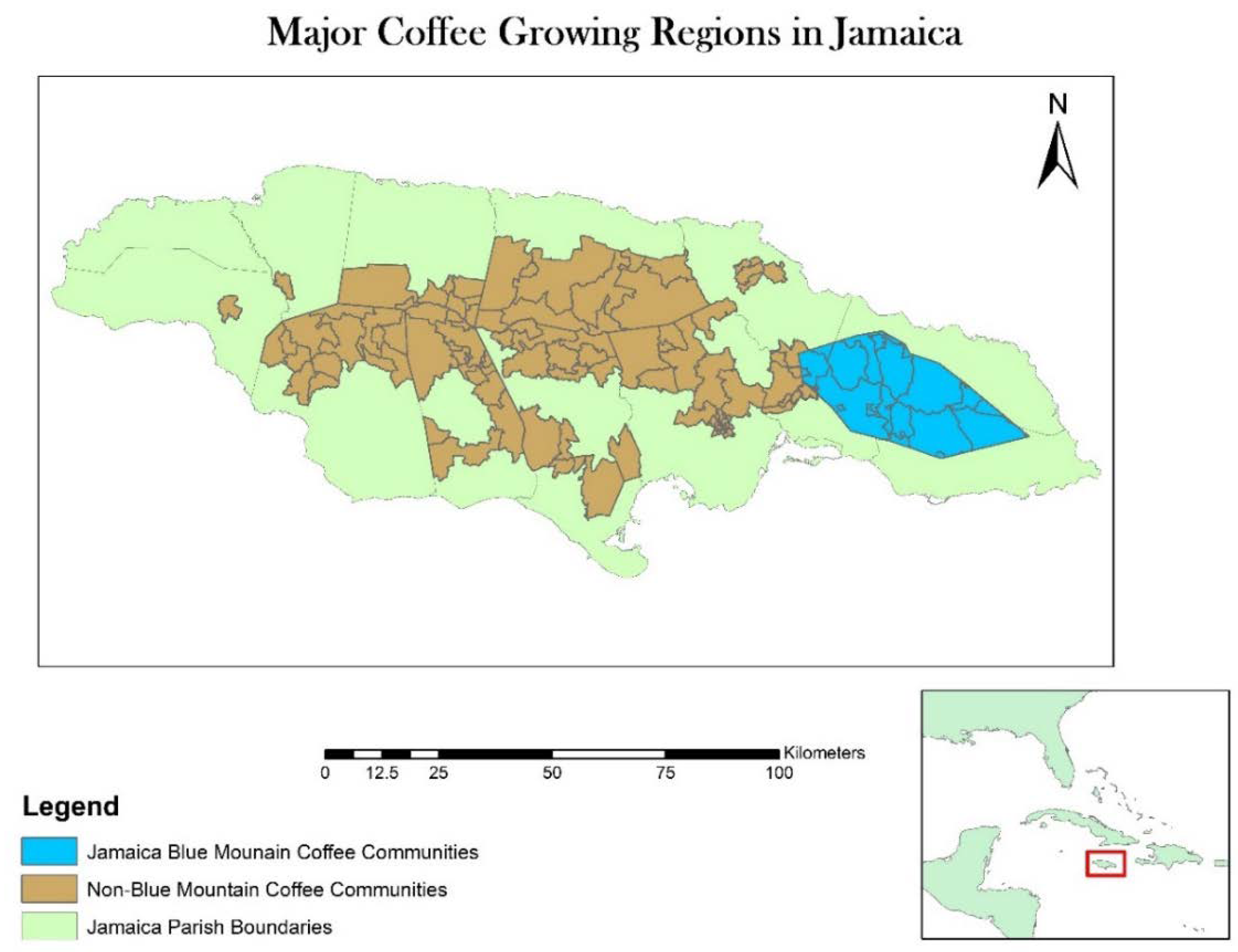
The Jamaican coffee industry (JCI) produces an Arabica varietal and has a longstanding reputation as being among the best coffee in the world [12]. Jamaican coffee is especially known for its Jamaica Blue Mountain (JBM) coffee brand which is cherished as a mild, smooth coffee with an earthy, deep aroma with hints of chocolate (and sometimes banana, cedar, and walnut) [13,14] and commands prices as high as US$60 per pound in some markets. Though the island has transitioned from an agriculture-based economy to one heavily dependent on the service industry (especially tourism), the niche that Jamaican coffee held among consumers has made it a valuable segment of the local agricultural sector. Employing several thousand people, the industry remains one of the island’s largest sources of agricultural foreign exchange earning US$16 million (over J$2.03 billion) in 2014 according to the Bank of Jamaica (2017). Coffee is typically grown in several regions across the island of Jamaica (see Figure 1).
Most coffee farms are located above 300 m on soils rich in organic material. The famous JBM coffee is grown in the Blue Mountains located in eastern Jamaica. With a maximum height of 2256 m, the range covers over 750 km2. JBM coffee is grown at elevations ranging from a low of 550 m up to 1600 m, with the best beans growing between 1100 and 1600 m. At these elevations, the higher quality Coffea arabica thrives; the berries mature more slowly and produce a drink with more delicate flavors than those grown at lower elevations. As a result, production is concentrated in the JBM region [15]. According to the Jamaica Agricultural Regulatory Authority (JACRA), about 80% of the island’s 5000 farmers are found in the Blue Mountains of eastern Jamaica. A smaller concentration exists in central Jamaica, and the balance is scattered throughout the hills of the island. The area outside of the Blue Mountain region is formally marketed as the Jamaica High Mountain region. However, for the purposes of this research paper, all areas outside of the JBM will be referred to as the non-Blue Mountain (NBM) region.
During the 1980s, relatively low production costs and access to government subsidies combined with high prices from large external demand made it possible for farmers to remain profitable regardless location. Since the 1990s, global production and competition in the specialty coffees market has soared and production costs have increased several-fold due to a severely weakened Jamaican dollar, increased impacts of pests and diseases and the evaporation of government subsidies. The regulatory authorities attempted to provide some stability by establishing price minimum to be paid to farmers per 60 lb. box of coffee at the start of each season. However, thousands of farmers have left the JCI and for many that remain involved, they do so because coffee production is part of their way of life. Production data obtained from JACRA indicated that almost 90% of Jamaica’s coffee production has been derived from the JBM region for the past several years (236,513 60-lb. boxes from the JBM region vs. 27,988 60-lb. boxes in the NBM region in the 2017–2018 crop year). A major influence driving this imbalance is the fact that farmers are paid almost twice as much for coffee grown in the JBM region as opposed to the NBM region.
The JBM brand has thrived in the last three decades of the 20th century, primarily in Japan. Its prominence is a stellar example of competitive advantage as it has been able to sustain profits that are greater than average for the global industry. However, over the past 15–20 years, the customer base has changed significantly: the loyal post–World War II customer base is being replaced by a new generation of coffee drinkers who are not as loyal, given a wider choice of specialty coffees and coffee blends. Combined with a steadily declining local currency driven by a stagnating economy, stakeholders in the JCI have had to adapt to the challenges of declining profitability due to rising production costs [15]. Anecdotal reports from field research in 2018 and 2019 indicate the need for the JCI to conduct more detailed data collection on yields, farm locations and other quantifiable data from production regions. Thus, the analyses conducted in this paper will be quite relevant not only to the JCI but other coffee enterprises worldwide that face similar challenges.
2.2. Geospatial Applications in Agriculture
The geospatial revolution has arrived on the farm. Applications range from mapping of various soil, water and nutrient components of agricultural land (e.g., [16,17]), land suitability assessment and multicriteria decision making (e.g., [15,18,19,20,21]), impacts of flood hazards (e.g., [22,23]) and precision agriculture (e.g., [24,25]) among others. The use of precision agriculture (PA), supported by GPS-oriented machines and variable rate of application, and drones to collect data with spatial resolution of less than a centimeter, the field of big data agricultural information is growing fast. However, the agronomic success of PA has largely been confined to large-scale, (relatively) flat land crops such as wheat, corn (maize), sugarcane, tea, and lowland coffee. Beyond this realm, and particularly in low income countries, the potential for economic, environmental, and social benefits of PA are largely unrealized because several practical barriers inhibit its successful implementation. These include the significant capital input to obtain the requisite information on field conditions, the prevalence of large numbers of small land holdings, lack of success stories, heterogeneity of cropping systems, infrastructure and institutional constraints and the lack of technical expertise knowledge and technology [26,27].
The research presented in this contributes to the realm of the economics of agriculture in GIS, something that has been considered essential for many, many years [24]. This paper provides a launching point for smaller scale agricultural producers—a point that is essentially the primary concern for all producers at all scales—profitability. The creation of this profitability model for the JCI enables producers to visualize expected returns and consequently make informed farm management decision. The model’s combination of site suitability and cost surfaces to generate a potential profitability surface using available information reduces the barriers to utilizing geospatial tools accessible to many of the large-capital intensive agricultural operations.
Landscapes, past and present, contain resources that are unevenly distributed, hence the value of GIS and other geospatial technologies in managing such resources. Site suitability and cost surface analyses attempt to quantify these variations for decision-making purposes. This paper does not focus solely on the environmental aspects but expands to other economic drivers of production. Most suitability (or cost) analyses assume technology as constant—a strong assumption, especially if we are analyzing a long period of time. Our study focuses on two recent crop-years; therefore, technology change should have no or minimal effect on the results present here.
Cost surface analysis (CSA) can be thought of as a generic name for a series of GIS techniques based on the ability to assign a cost to a point/line/area in a vector dataset or each cell in a raster map, and to accumulate these costs by travelling over the map [28]. CSA can incorporate relevant properties of the terrain being studied and allows rules to be set based on distance, time, energy, and other costs to create a multi-criteria cost surface [28,29]. One advantage of this approach is that it is possible to tailor the priority or weighting of the various cost factors as one desires, making it useful to researchers interested in diverse social, temporal, and regional settings. These surfaces can then be used to inform a multiplicity of decisions. Examples of CSA can be seen in many fields of study, ranging from ecology (e.g., [30,31]), planning and engineering [32], archaeology (e.g., [28,29]) to agriculture [33]. According to [29], another advantage is that, while multi-criteria cost surface analysis allows flexibility and variation between cases, the concepts underlying it are straightforward and universal to its application. This universality ensures that, while there is variation, different studies are still comparable, furthering its cross-cultural applicability. Building on this concept, a profitability model which incorporates a revenue estimate and a CSA has the advantages of CSA while identifying both areas of least cost and highest profitability.
CSA involving profitability modeling is highlighted in [33,34]. Bateman et al. [34] creates a model of timber production for two species (Sitka spruce and beech) utilizing both statistical modeling and GIS approaches. While rigorous in its yield modeling, this work did not consider production or operational costs, which limits the ability to assess actual profitability. McConnell and Burger [33] takes things a step further to consider both components as predictors of profitability. They combined PA and conservation approaches in order to identify lands that were available to enroll in USDA conservation programs and calculate potential profitability for utilizing land in and out of two conservation programs. They illustrate the utility of a profitability tool to model the financial opportunities associated with combining crop production and available conservation incentive programs [33] (p. 350). A key component in this profitability tool is the availability of spatially explicit yield data (ibid.)—this enables one to visualize a variety of profit surfaces related to agricultural production under various scenarios.
Bazzi et al. [35] and Marinoni et al. [10] provide insight on the mechanics and utility constructing profit maps at various spatial scales. With the technological advances in PA that have made yield maps accessible to farmers, ref. [35] investigates the utility of creating profit maps rather than just yield maps as well as the effect of various interpolation methods on the results of these maps. Since yield variability has rarely been correlated with profit variability [35,36] analyzed yields for four crop areas in Paraná, Brazil which grew either soybean or corn in order to create their profit maps. As with other efforts at creating profit maps, they acknowledged the impacts of variation in agricultural prices on profit results (and the consequent ‘best time’ to sell a harvest. It was assumed that all crops were sold at the end of the harvest to maintain consistent comparisons. The shape of the profit maps was strongly impacted by the yield map results. However, all fields studied showed large profit variations that would not be easily found by analyzing a yield map alone [35] (pp. 391–392). Marinoni et al. [10] considered a more expansive spatial scale than [34]—the entire continent of Australia. At the core of their creation of maps of agricultural profitability was a database (SQL Server) that stored information about revenues and production cost for a variety of agricultural commodities for various spatial entities. This database architecture allowed for the inputting of heterogeneous information collected by a variety of institutions across different scales. They argued that such a structure would allow information to be queried, processed, and visualized in a GIS environment. It also facilitated the production of profit maps in the future using updated economic information and geospatial datasets. According to [10], this would help end users, policy makers, and researchers understand profit trends in time and across space as well as address issues such as climatic variability, changes in land use and demographic developments.
Among the challenges in creating profit maps noted by [10,35] was that the final accuracy of a profit map is influenced both by the spatial prediction from the yield map and the quality of the economic data, especially temporal inconsistencies for cost information. A compound challenge is that final profit maps have a significant in-built uncertainty and error that is often not made explicit in the results. Some of these challenges are addressed in our study by using a proven coffee suitability model for the study area [15] and incorporating price information sourced directly from the coffee regulatory authority. The issue of inherent error can be addressed at the source of the various datasets, something beyond the control of the researchers. However, the challenge of creating a model that can be regularly updated is a clear need to be filled in our web-based/internet-connected society. In combination with the many other variable incorporated in the creation of this model, the key to realizing the potential in these programmatic opportunities, i.e., CSA and profit models is helping producers visualize spatially explicit economic and environmental tradeoffs [33] (p. 351).
2.3. Methods: Data Collection, Analysis, and Results
This section provides an overview of the steps involved in producing the models of profitability for the JCI. The approach to the methodology was guided by [10]. A summary of the entire process is laid out in Figure 2 below.
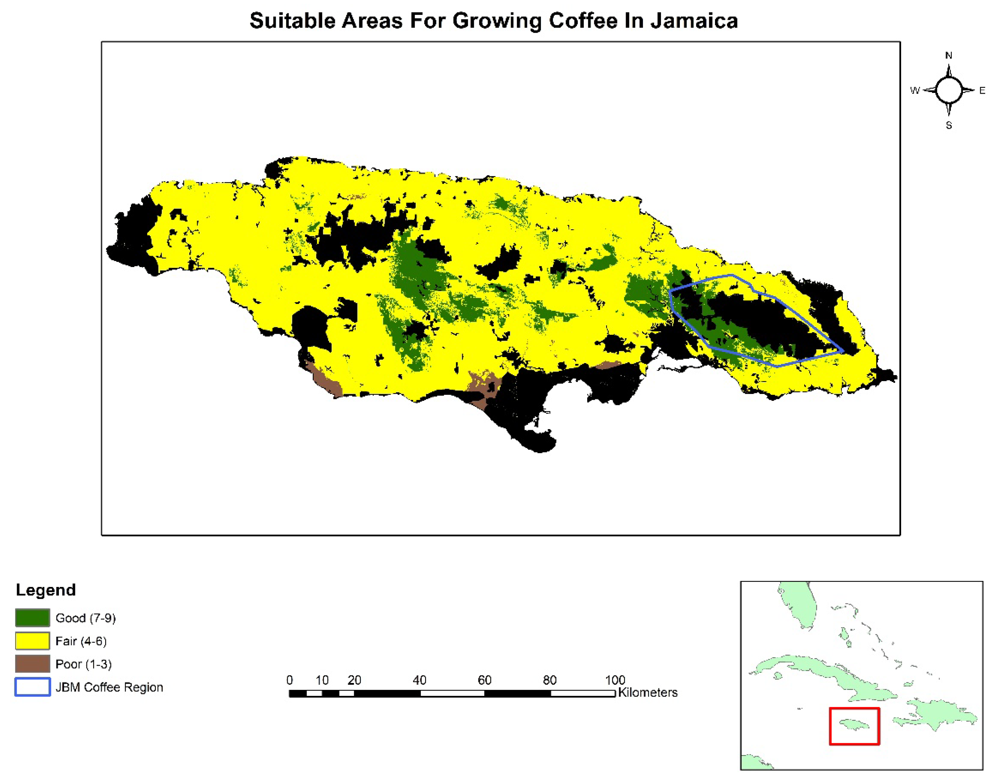
This profit model incorporated a previously developed suitability model which utilized the analytic hierarchy process to integrate the expert knowledge of local coffee stakeholders [15]. Eight biophysical and infrastructure variables (elevation, temperature, geology, soil type, slope, precipitation, distance to roadways, and distance to waterways) were weighted based on importance to coffee production in Jamaica. Each criterion in the suitability analysis was then reclassified on a scale of 1 (worst) to 9 (best) based on their suitability for coffee production. The most suitable areas for growing coffee were to be found in the mountainous core of central and eastern Jamaica and least suitable areas were to be found on the southern and northwestern coastal plains of the island. A generalized version of the suitability map is presented in Figure 3 below.
2.3.1. Development of Profitability Model
Profitability is defined as it simplest as income minus operating or production costs. However, in the context of agricultural production, profitability can be further defined in a few more ways: a farmer may or may not include their own labor as an input costs; depreciation of equipment can be included in operating costs; so too can debt/interest payments. Further still, the rate of return on farm investment can be compared to working outside of the farm to assess whether or not a farm is profitable [37,38]. In this paper, the researchers define profitability as the result of income minus direct production costs. This straightforward approach enables us to make use of the currently available datasets for this project as well as provide a standard base upon which the relevant coffee stakeholders can incorporate other desired costs or benefits.
The formula used to calculate profitability is
where Y is the profit (or loss) in US dollars per unit area in area i at farm gate; Yld is the coffee yield (in 60 lb. boxes) per unit area; L is the percentage crop loss (including loss due to pests and diseases) per unit area; P is the price paid per 60 lb. box of coffee cherry (price per box); SYld is a yield scale factor derived from the suitability model in [15]; C is the production costs (per unit area); CT is the contingency cost (accounting for various unforeseen expenses) per unit area; SC is the production scale factor derived from the suitability model in [15]. The values for Yld, L, P, C and CT were all derived from official coffee production cost estimates published by JACRA and detailed in Supplementary File S1 of the supplementary materials. JACRA compiles this information based on data from field experiments on ideal production conditions as well as annual surveys of prices for the various input materials (fertilizers, labor, equipment etc.).
The yield and cost scale factors (SYld and SC) were utilized as a proxy measurement of the variations in coffee yields and production costs experienced by producers on the ground. Due to the variable nature of production yield across the island, the researchers consulted with field extension officers of the JACRA to determine an appropriate interval for the scale factors. After presenting preliminary analyses of the effects of several possible intervals it was determined by the field officers that a scale interval of 5% would most closely represent the realities and experiences of coffee producers [39]. The scale factors follows the suitability scale presented in Figure 3, with areas rated as good (suitability of 7–9) being assigned a scale of 1.0 (maximum potential yield and base level of cost); areas rated as fair (suitability of 4–6) are assigned a scale of 0.95 (95% of maximum potential yield) and 1.05 (105% of base cost level); areas rated as poor (suitability of 1–3) are scaled at 0.9 (90% of maximum potential yield) and 1.10 (110% of base cost level). In other words, areas with ideal growing conditions face no reduction in maximum estimated yield or increase in production costs. As suitability for the production declines, the scale factors correspondingly reduce maximum potential yields and increases production costs for the crop. The unit area i represents one grid cell of the profitability model which has a spatial resolution of 30 m. Therefore, each cell represents 900 m2 (derived from 30 × 30 m raster grid cells). This value can also be expressed as 0.09 hectare or 0.222 acre.
To showcase the utility of this research, two coffee years were selected for modeling in consultation with JACRA—the 2016–2017 coffee year, where prices reached record highs in recent history, and the 2018–2019 coffee year where prices paid to farmers fell significantly compared to the record high prices but were closer to average prices in recent history in the local industry. These two years were selected based on the availability of the data and for exploring the impacts of the significantly different prices being paid on coffee production profitability in the island. As outlined in Section 2.1, the JACRA established price minimums paid to farmers per 60 lb. box of coffee for each season. The setting of these prices is informed by production levels from the previous coffee year and dialog with major buyers of the coffee cherries across the island [39].
The modeling of coffee profitability in this paper carries certain assumptions: (i) coffee producers are cultivating ‘pure stands’ of coffee, with fully mature trees and maximum production, while following the JACRAS’s best practices; (ii) producers are profit-maximizers, agents, and price-takers, however they are not counting their own ‘sweat equity’, i.e., they do not include their own labor as part of the production costs; (iii) no stock formation—all crops are sold at the end of the harvest to maintain consistent comparisons; (iv) producers have equal access to necessary farming technologies; and (v) travel costs are constant across the study area.
2.3.2. Data Collection
In order to create the coffee profitability model using the formula above, a variety of information needed to be collected. Table 1 below summarizes the information collected for this research project.
Detailed information on various income estimates and production costs were obtained from JACRA [39]. The agency maintains a proprietary database of production cost estimates in order to provide recommendations and updates to various stakeholders in the local coffee industry. This information ranged from estimates of number of man hours required to perform various on-farm tasks, to amounts and costs for various herbicides, fertilizers, and insecticides used throughout the coffee year, to transportation and harvesting costs. Please see the supplementary information provided in the appendices for details on the variables used. The coffee suitability model for the island of Jamaica was obtained as a raster dataset that portrayed the suitability of the land area for the island for growing coffee on a scale from 1 (least suitable) to 9 (most suitable). The model used eight biophysical and infrastructural variables to evaluate the island of Jamaica for suitability for coffee production. A comprehensive description of the model’s data sources and creation can be obtained from [15].
As mentioned above, two years were selected for modeling profitability in the JCI. In 2015 there was a significant decline in coffee production island-wide leading to a shortage of product for the export market. Competition for the scarce crop among dealers saw prices offered to farmers rise significantly across all regions, and reached a peak in the 2016–2017 coffee year (as high as US$94/J$12,000 per box in JBM regions and US$39/J$5000 in NBM regions). However, as more and more coffee entered the local market, there was oversupply of coffee and prices fell precipitously. By the 2018–2019 coffee year, prices offered to farmers were almost half what was offered just two years earlier (on average US$38/J$5000 per box in JBM regions and US$26/J$3500 in NBM regions). This rapid change provided a great test case for this research endeavor and thus, these two years were chosen for modeling profitability in the local industry.
2.3.3. Data Preparation
After obtaining the variables needed to calculate profitability, they were formatted for use for the model. All values recalculated to align with the areal unit/measure being used and costs were kept in their values of Jamaican dollars until final results were calculated. The yield scale and production cost scale factors were created from the suitability model. These scale factors were used as a proxy for actual yield monitors that one would find in advanced agricultural enterprises [35] (p. 386). In consultation with extension officers at JACRA, the suitability model was first divided into three groups and then a scale factor applied to each group. It was recommended that 5% would be an appropriate scaling factor to use for this model [38]. As noted in Table 1 above, coffee yields and production costs were adjusted as follows: areas rated 7–9 were assumed to obtain maximum yield and incur base level production costs; areas rated 4–6 saw a 5% decrease in yields and a 5% increase in production costs; and areas rated 1–3 saw a 10% decrease in yields and a 10% increase in production costs.
In order to effectively manage this significant dataset, a file geodatabase was created using the ArcGIS suite of software. The program ArcCatalog was used to create the geodatabase and set up the necessary schema and domain attributes. The raster dataset of suitability values had a 30 m cell size and was converted to a point vector dataset in order to facilitate easier attribute table management. This conversion resulted in just over 9 million data points of coffee suitability for the island. After validating the spatial integrity of these points, fields were added denoting whether or not the point was located in the JBM region (price differentiator) in both string and binary formats. The attribute table of this dataset was then exported for further processing using Python code. The processing used the Geopandas and Numpy libraries to handle the computation of the profitability for all the 9 million data points. The results were exported as a CSV file and later incorporated into the geodatabase.
3. Results
Once all the relevant variables were entered in the database, the profitability formula was run to calculate estimated profit or loss for each data point across the island (see Figure 3, Figure 4, Figure 5, Figure 6 and Figure 7). Across both model years, the primary changes surrounded the price paid per 60 lb. box of coffee. Most of the other variable remained fairly constant for both income and production cost calculations. The contingency factor used in the calculations was 5% (per JACRA recommendations). The outputs of these calculations reported income, production costs and profitability with and without the scale factors in Jamaican dollars. These results were converted to US dollars using the average exchange rate for the relevant coffee year. The final outputs were converted first to a comma separated value (CSV) file, then the CSV file imported as a database table back into ArcCatalog. This table was joined to the original point dataset, giving the researchers profitability information across the island of Jamaica.
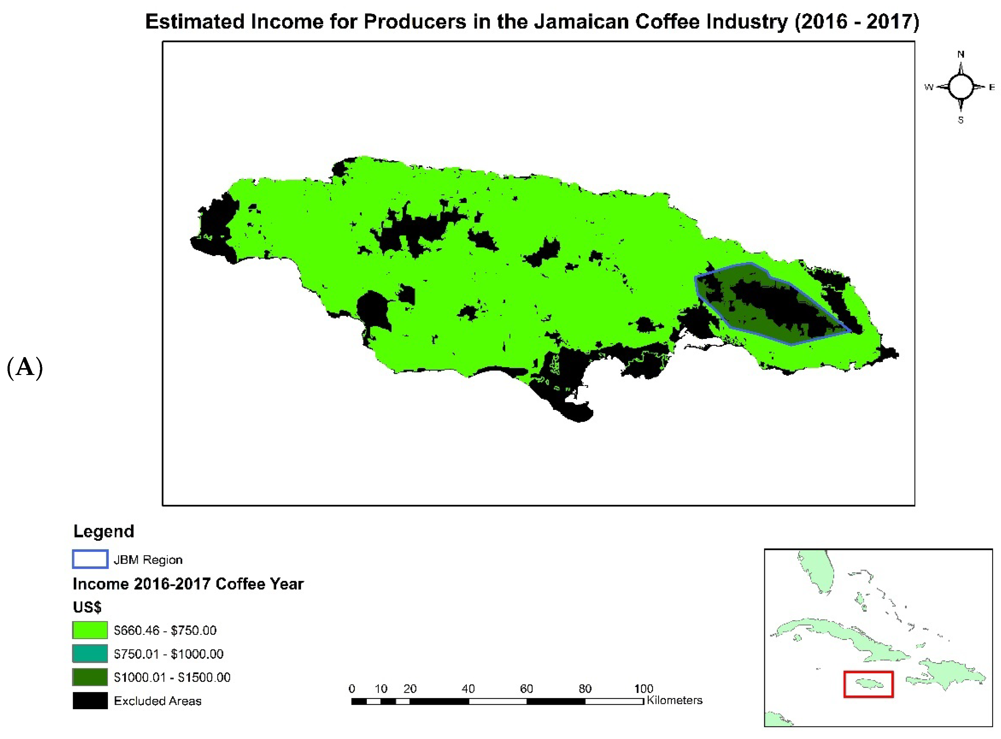
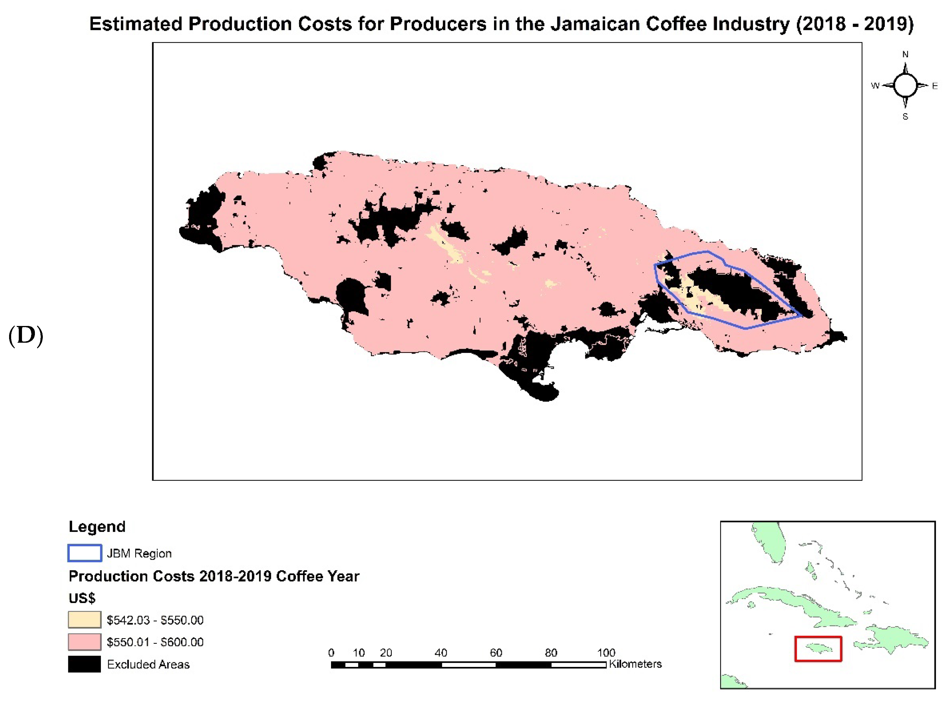
For better visualization and rendering, the results were converted to raster datasets for each modeled coffee year. Figure 4 presents a visualization of the income generated and production cost surface across the island while Figure 5, Figure 6, Figure 7 and Figure 8 display the profitability results for the 2016–2017 coffee year and 2018–2019 coffee year across the entire island as well as the four coffee extension regions used by JACRA.
Table 2 below provides a summary of the key statistics resulting from the profitability calculations in three groups—overall values for the island, JBM and NBM regions, and the four extension regions for each of the model years.
4. Discussion
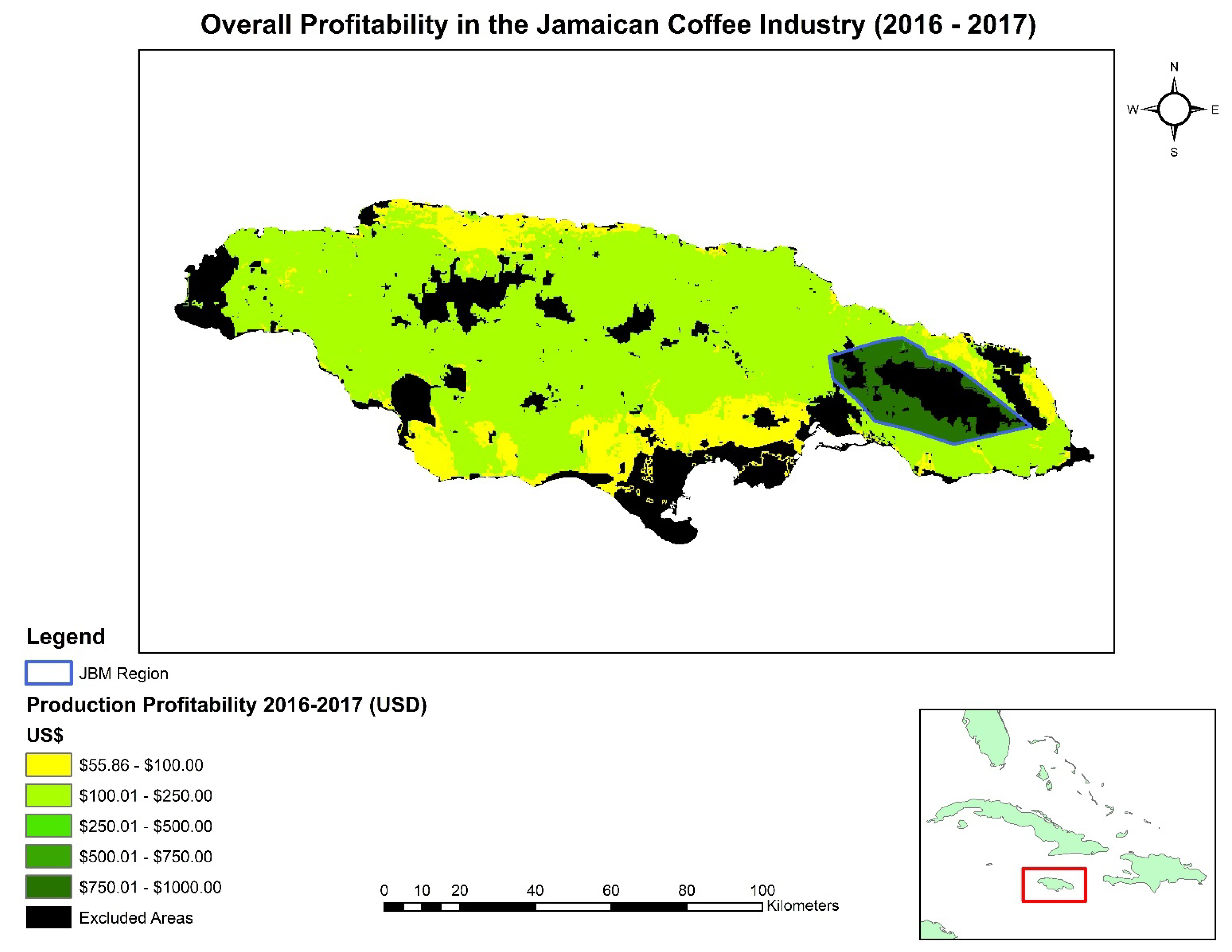
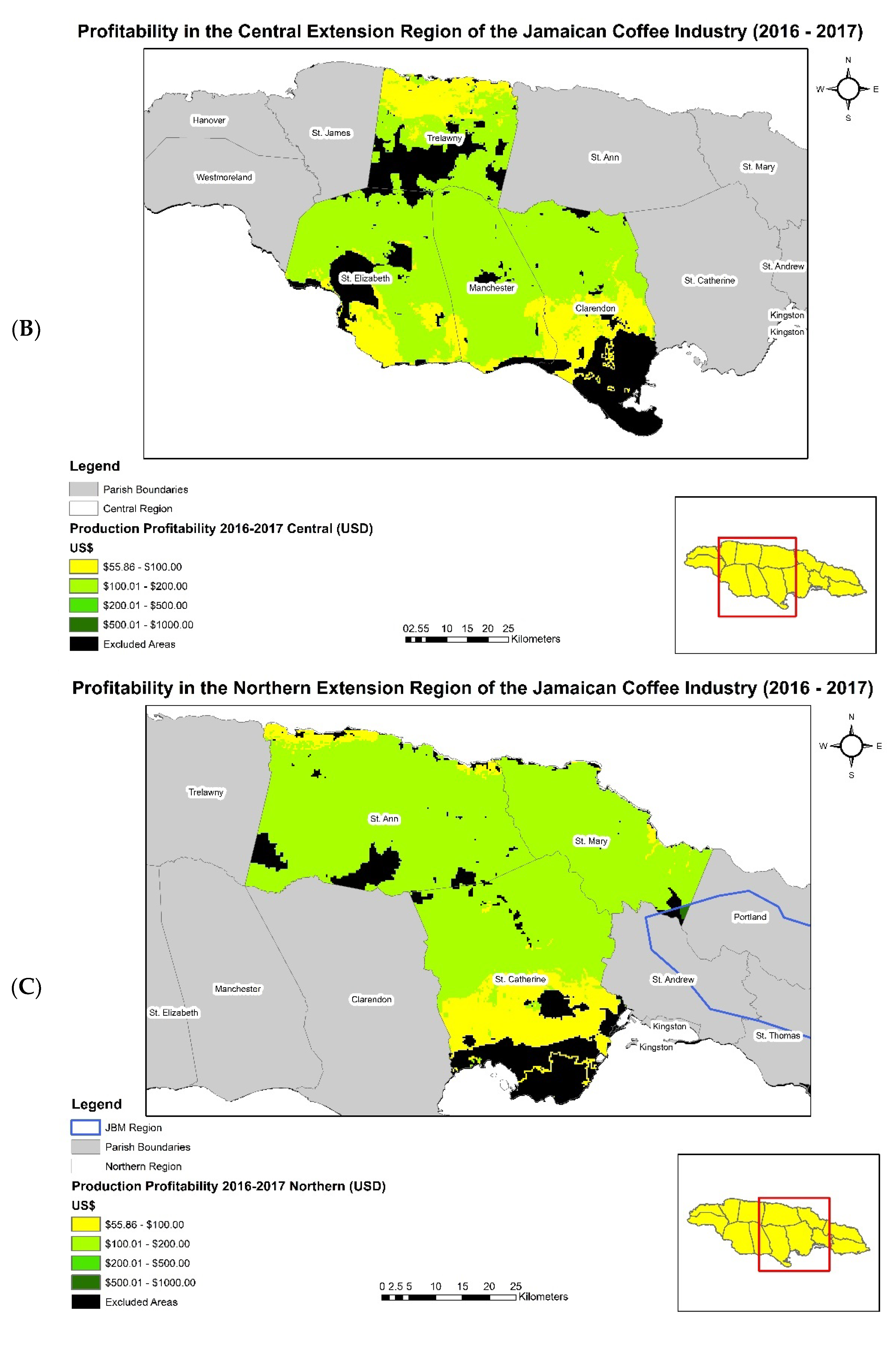
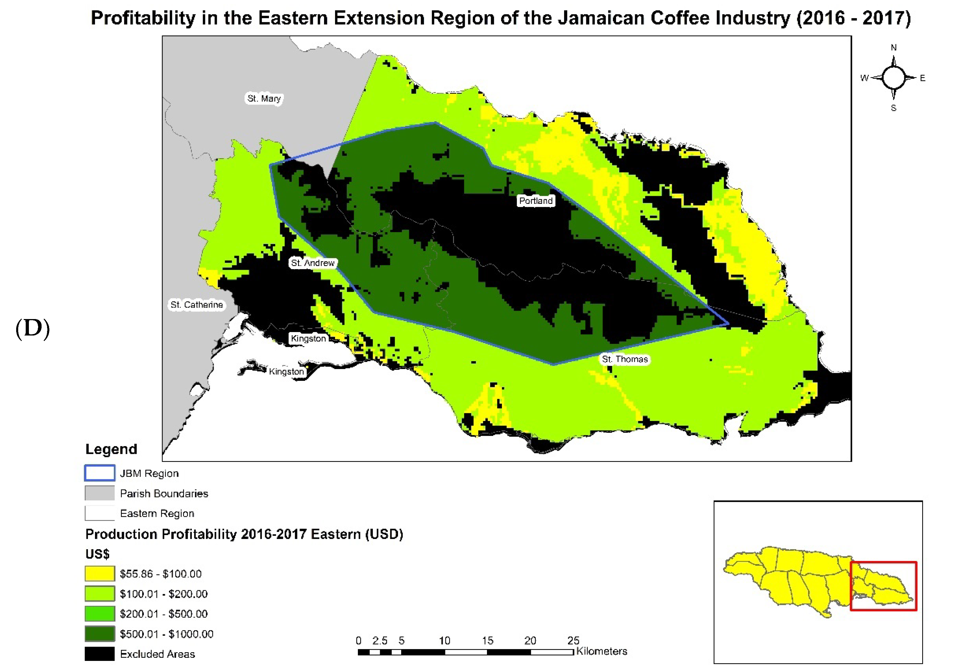
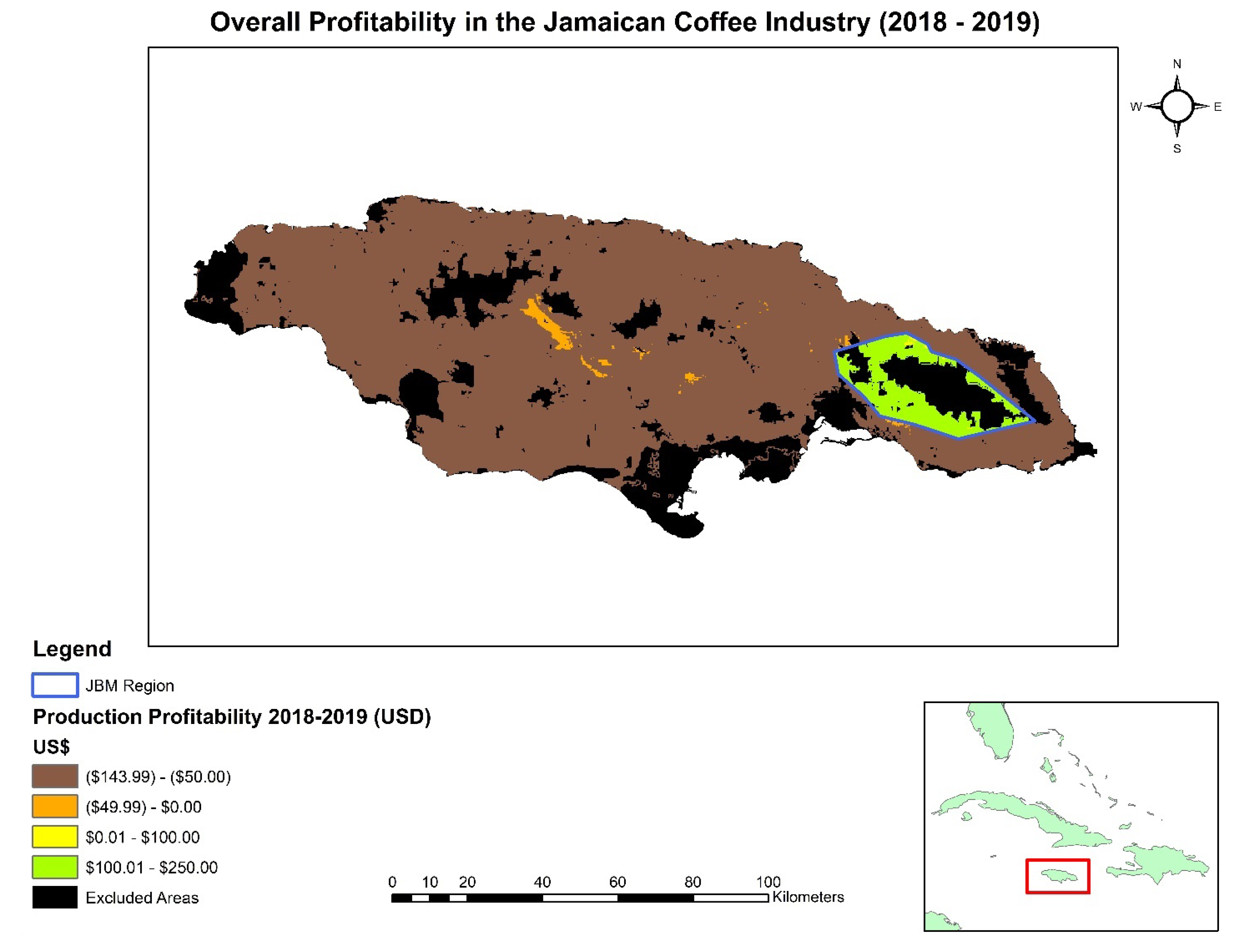
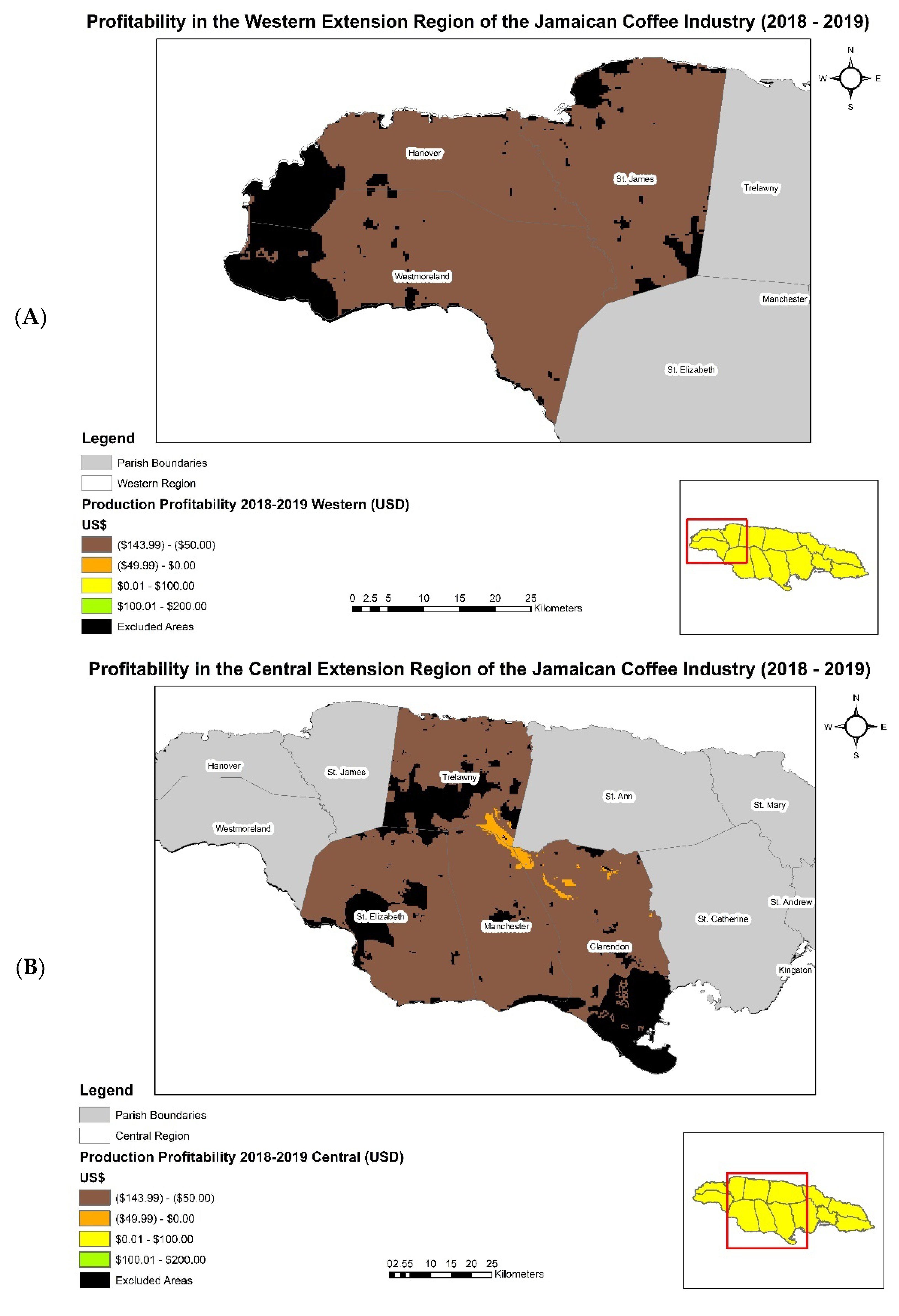
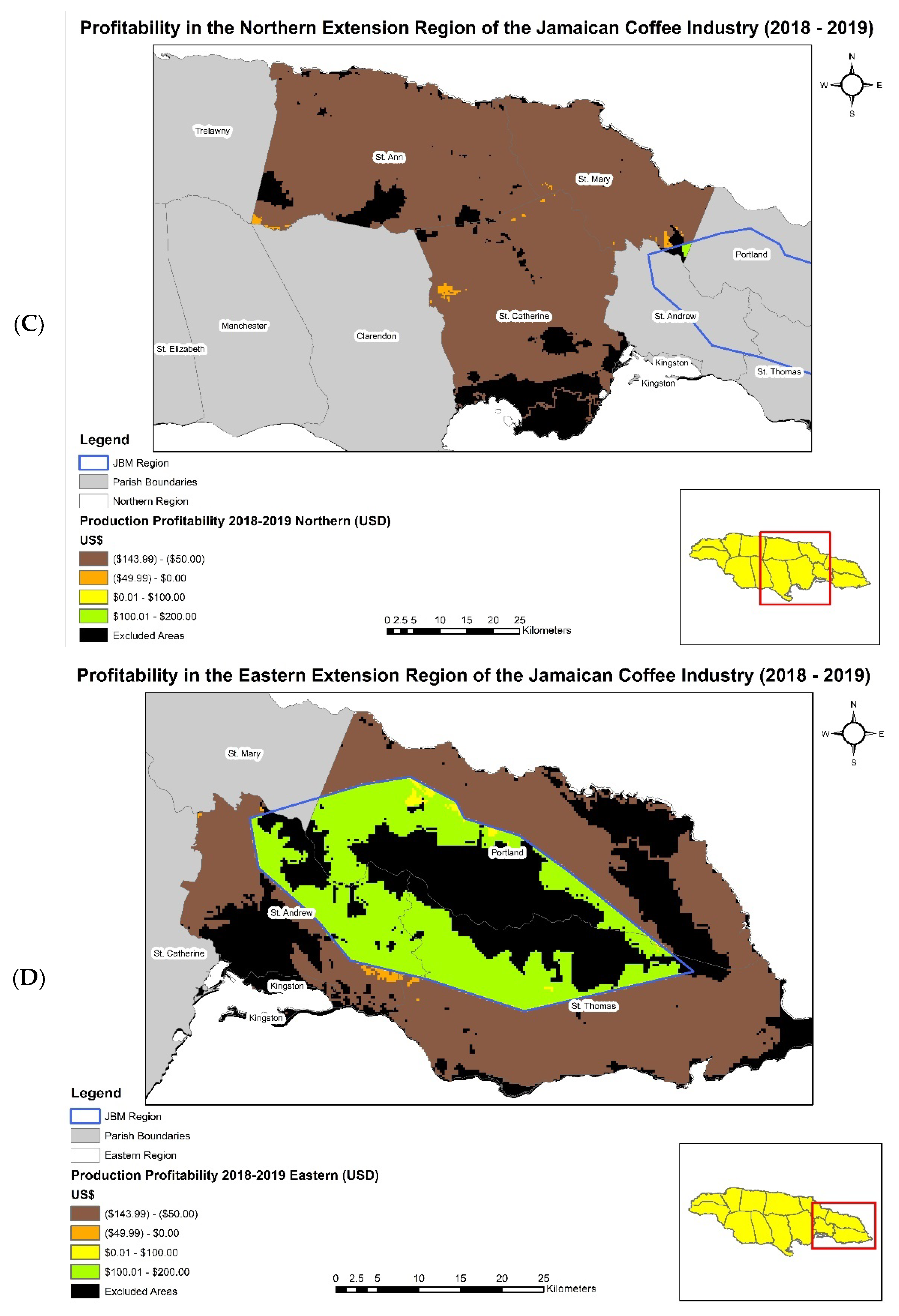
The record high prices paid to farmers for their coffee in the 2016–2017 coffee year is clearly reflected in the profitability results for that year. Figure 5 reveals that all areas of the island, even areas that would be considered unsuitable for viable production would return a profit if coffee were cultivated, harvested and sold. Taking a closer look at the various sections of the island, the eastern extension region (Figure 6D), which includes the JBM coffee region returned the greatest profit margin while the western, central, and northern extension areas appeared to return a much lower (but still positive profit margin) as shown in Figure 6A–C. The contrast with the 2018–2019 coffee year, where prices paid to farmers fell significantly is stark and apparent—this decrease in income is reflected in Figure 4C. In Figure 7, we can see that all areas of the island, except for the JBM region, now experience losses. Zooming into the various extension region maps in Figure 8A–D, coffee producers in the western, central, and northern extension areas were expected to incur losses for this coffee year, while the eastern extension area would only realize a modest profit margin in the JBM region and losses outside of this area.
The visual depiction of these results is further supported by the statistics presented in Table 2. Production costs remained fairly constant across the island for the two modeled years at approximately $575 per unit area (or just under $6400 per hectare/$2600 per acre), with slight variations due to the change in exchange rate and the impact of the scale factors derived from the suitability ratings. In the 2016–2017 coffee year, the mean income is estimated to be $723 per unit area (or approximately $8033 per hectare/$3257 per acre) but this falls to $483 per unit area (or approximately $5366 per hectare/$2175 per acre) for the 2018–2019 coffee year.
Surprisingly, the NBM income had a smaller reduction than the JBM for the period, a drop of 31.5% compared to 51.1% of the JBM. The difference in prices paid to farmers in the JBM and NBM coffee region was the driver behind this notable difference in income and consequently profitability in both modeled years. Income in the JBM region was almost 100% greater than the mean in the 2016–2017 coffee year and almost 50% higher than the mean for the 2018–2019 coffee year. While income in the NBM coffee region was 4% and 2% lower than the mean for the respective years. Considering that production cost is quite similar among regions, the resulting profitability then is no surprise. Farmers in the JBM region were estimated to realize a profit of $847 per unit area (or $9411 per hectare/$3815 per acre) and NBM farmers obtaining a profit of $111 per unit area (or $1233 per hectare/$500 per acre) for the 2016–2017 coffee year. The sharp drop in income (coffee prices fell by US$38.02/J$5000 in the JBM region and by US$11.40/J$1500 in the NBM region) in the 2018–2019 coffee year meant that farmers JBM region would achieve on average a profit of $130 per unit area (or $1444 per hectare/$585 per acre) and NBM farmers would realize losses of $98 per unit area (or $1088 per hectare/$441 per acre).
The profitability model results clearly highlight the challenges to economic feasibility in the JCI. Production anywhere outside of the JBM region is a low profit undertaking and this continues to drive the concentration of coffee farmers into the JBM region. Considering that the 2017 GDP per capita for Jamaica was just over $5100 (World Bank Group 2019), a producer would need to cultivate at least 25 acres or 10 hectares in the NBM region to achieve the mean GDP level in the country as compared to 1.3 acres or 0.5 hectares in the JBM region in the 2016–2017 coffee year. However, the results for the 2018–2019 coffee year paints a grimmer picture. With the sharp decrease in prices paid per box to producers, a farmer would need to cultivate at least 8.7 acres or almost 3.5 hectares in the JBM region to achieve the mean GDP level for the island. With losses being incurred with every unit area being cultivated in the NBM region, farmers would need to implement measures to further reduce production costs or increase revenues in order to achieve the nation’s mean GDP level.
The implications of these numbers are clear: in ‘good’ years, when there is limited production and prices rise there is money to be made, but when farmers increase production in response to this, then oversupply results in lower prices and economic loss—the classic supply and demand curve reflecting the point made by [35] on the impacts of variation in agricultural prices on profit results (and the consequent ‘best time’ to sell a harvest). However, with the conventional coffee market saturated with coffee for the last several decades and the specialty market becoming ever more crowded, stakeholders in the JCI may need to consider the best route forward in order to remain economically viable, particularly at the farmer level. Considering that a significant proportion of the island’s small farmers cultivate less than one hectare of coffee, the attraction to remain in coffee production is likely to continue waning and decreasing the number of stakeholders in the JCI.
One possibility may be the creation of production quotas (similar in concept to the international coffee agreements of the 1960s through to the 1980s in the global coffee market). Such a mechanism may include a provision allowing for the suspension of quotas if prices remain high, and their reintroduction if prices became too low [40]. This would be useful since most producers lack the ability to process and store their harvest and sell at time when prices are higher. Some producers may consider diversification away from pure coffee production if this crop has become a money-losing venture. The researchers would dare say that unless farmers are able to ally themselves with other areas of the coffee value chain (particularly the export or resale of green or roasted coffee) or increase their production to gain greater economies of scale, then it may be more feasible to focus on diversification to other crops or livestock.
Conversations with representatives from JACRA [39] revealed that the prices for the 2016–2017 year was considered unsustainable as it was fueled by a severe shortage in supply. Current prices reflect the glut in the market due to oversupply of green bean coffee to purchasers. They estimate that a market correction to stable prices of approximately J$7000 (US$53.5) and J$4000 (US$30.5) per 60 lb. box for JBM and NBM coffee cherries should occur over the next few years. Even at these prices, it remains very clear that Jamaica’s current small farmers engaged in coffee production, those cultivating under 0.4 hectare or 1 acre of coffee will be engaging in a money losing proposition depending solely on coffee. During on the ground conversations with farmers, increasing the prices paid to the farmer is a popular proposition. However, this ignores the reality that there is a decreasing demand for JBM and other Jamaican coffees from their primary market of Japan. Efforts that have been made to expand the market for Jamaican coffee in the USA, Europe, and Asia must be reinforced in order to viably increase the prices paid per box, and consequently the income that can be received by the producer. In the most extreme case, with limited government resources to support industry stakeholders, one may consider solely focusing efforts on the JBM brand. In this high cost production reality of growing coffee in Jamaica, unless farm gate prices increase to above breakeven levels (at least US$30.5/J$4000 per box), losses will continue to be experienced by many coffee producers.
For producers seeking to go beyond the mean GDP per capita, it is instructive to observe that the land area requirements are significantly greater in the NBM region. Larger farms will incur other costs not considered by this model (dedicated farm vehicles, full-time staff, etc.) that will potentially reduce profitability. All else being equal, it is rare for production costs in agriculture to remain stable. Decreases in production costs are often realized from either incorporating some form of labor-saving technology, especially in larger (over 20 Ha) enterprises or realizing economies of scale by increasing production volume relative to input costs. In Jamaica, as in many other developing nations, inflation, and a depreciating local currency have a strong role in driving increasing production costs rather than an increase in actual farm needs. Agricultural inputs such as fertilizers and pesticides are often imported using foreign currency, and depreciation leads to making imported products more expensive without a corresponding increase in value for local goods and services. This implies that especially for producers in the NBM region, locating in the few areas of high suitability and crop diversification remain the clearest path to profitability. Some farmers may consider pursuing a cooperative model in order to gain some benefits from an increased economy of scale. However, weak formal institutions to enforce contracts and agreements and lack of trust amongst peers present significant challenges to this approach (see [41,42] for more on these challenges to this approach).
In our analyses of profitability potential for the JCI, we have seen that many areas of the island are likely to operate at a loss, given the most recent farm-gate prices for coffee. The fluctuations in market prices for this commodity means that farmers need to plan and implement efficient use of input resources. One strategy that is widely implemented across tropical coffee farms in Jamaica and around the world is the use of fruit or hardwood trees for shade [42,43,44,45]. The revenue from these trees can support the goals of farm profitability with the additional benefit of forming sustainable agroecosystem—an important tool for habitat restoration efforts [45]. However, this common approach does violate one key model assumption—that of cultivating pure stands of coffee. The assumption of best practices is a simplification necessary to represent the current official standard of production and the official data for cost and yield. In future work, the profitability model could be improved to accommodate the presence of intercropping if data for the secondary crop is available. Moreover, the present model should be seen as an unrestricted coffee profitability model as coffee trees are not competing with other crops for area. Another crucial consideration in applying the results of this research is assessing real world yield estimates with model estimates in order to ground stakeholder expectations of profitability. Mechanization is often discussed as a means of increasing efficiency, but in the case of the JCI, steep slopes and high equipment costs generally limit machinery to transportation of inputs and produce to and from the farm and utilizing handheld machinery in the fields. A major consideration that will have long term impact on profitability is the threat posed by climatic changes. Many sources have documented these actual and predicted effects, which range from increased ranges for pests and disease to disruption of favorable growing conditions, all of which will affect profitability (see for example [9,46]).
5. Conclusions
This research presented local-level models of profitability from coffee production in Jamaica for the 2016–2017 and 2018–2019 coffee years. With the saturation of the conventional coffee market, one might expect significant specialty coffee brands to consistently return profit year after year. However, this is not the case. With increased competition, variable supplies and changing consumer preferences, prices paid to farmers fluctuate—sometimes significantly over a relatively short period of time. While always an enterprise fraught with risk, these wide price fluctuations add an element of risk that many stakeholders, particularly small farmers are no longer willing to endure. This is a tale that plays out across multiple agricultural crops at several scales all around the world. The geospatial models created in this research provide an opportunity for those involved in agriculture at smaller scales to take advantage of the PA toolsets available to larger farmers in order to support an informed decision-making process. The methodology presented here provides a fairly flexible method for replication in regions/countries where detailed yield monitoring is uncommon or unavailable.
The researchers believe that this paper provides a means to address a number of the challenges to geospatial applications in agriculture, most notably small farm sizes and the technical expertise to generate such a model. Based on the researcher’s field experiences, producers will have an idea of how well (or not) the coffee year is going but many do not keep a detailed record needed to calculate profit or loss in a given year by smaller areas. Furthermore, the model presented here can be used to plan new producing areas by offering a reference for potential profitability. Thus, the detailed results of this model might be valuable as a reference point for Jamaican coffee farmers, and consumers of Jamaican coffee worldwide. There remains a number of valid obstacles, particularly the issue of crop heterogeneity and any number of infrastructural and institutional constraints not accounted for in this model. While the model assumes that farmers are following recommended practices by extension officers, it is fair to assume that a significant proportion of producers are more risk averse, accepting lower yields in order to have a more diversified farm base instead of pursuing higher yields and dealing with the variable nature of coffee prices over time.
This paper has demonstrated the viability of modeling potential profitability in a specialty agricultural enterprise. We have also shown the utility that this model has for coffee stakeholders, but particularly for producers in the island of Jamaica. This model has the potential to be incorporated into a spatial decision support system that can be used for planning purposes by regulators, investors, and other stakeholders. It also has the potential to be transformed into a web-based or mobile application for a crop profitability calculator, where users could personalize results with their own variables for yield, price, and production costs and obtain up-to-date and spatially-explicit profit estimates in their area(s) of interest. Geospatial application such as this model can enable underserved farmers to receive the benefits of the new technologies that are promoting higher gains to larger and more capitalized farmers—a situation faced not only by Jamaican coffee producers but by small farmers around the world.
Supplementary Materials
The following are available online at https://0-www-mdpi-com.brum.beds.ac.uk/2077-0472/11/2/121/s1, Supplementary File S1: Detailed profitability calculation values; Supplementary Table S1: Key Profitability Statistics for the 2016–2017 and 2018–2019 coffee years.
Author Contributions
Conceptualization, M.M. and G.G.; methodology, M.M. and G.G.; software, G.G.; validation, M.M. and G.G.; formal analysis, M.M. and G.G.; investigation, M.M. and G.G.; resources, M.M. and G.G.; data curation, M.M.; writing—original draft preparation, M.M. and G.G.; writing—review and editing, M.M. and G.G.; visualization, M.M. and G.G.; funding acquisition, M.M. All authors have read and agreed to the published version of the manuscript.
Funding
Field data collection for this research was funded by a research grant from the University of North Alabama.
Data Availability Statement
Restrictions apply to the availability of these data. Data was obtained from JACRA and are available by contacting [email protected].
Acknowledgments
The authors wish to specially thank Gusland McCook, Gary Watson, and Tiffany Hedge-Ross of the Jamaican Agricultural Commodities Regulatory Agency for their help in reviewing and fine tuning the parameters for the model presented in this research. G.G. work in this project was supported by the California State University Agricultural Research Institute Grant number 21-04-107.
Conflicts of Interest
The authors declare no conflict of interest. The funders had no role in the design of the study; in the collection, analyses, or interpretation of data; in the writing of the manuscript, or in the decision to publish the results.
References
- Pendergrast, M. Uncommon Grounds: The History of Coffee and How It Transformed Our World; Revised Version; Basic Books: New York, NY, USA, 2010. [Google Scholar]
- Pendergrast, M. Uncommon Grounds: The History of Coffee and How It Transformed Our World; Basic Books: New York, NY, USA, 1999. [Google Scholar]
- Kaplinsky, R.; Fitter, R. Who Gains from Product Rents as the Coffee Market Becomes More Differentiated? A Value-chain Analysis. IDS Bull. 2001, 32, 69–82. [Google Scholar] [CrossRef] [Green Version]
- Kaplinsky, R. How can agricultural commodity producers appropriate a greater share of value chain incomes? In Agricultural Commodity Markets and Trade: New Approaches to Analyzing Market Structure and Instability; Alexander, S., David, H., Eds.; Food and Agricultural Organization: Northampton, MA, USA; Edward Elgar Publishing Inc.: Northampton, MA, USA, 2006; pp. 356–379. [Google Scholar]
- Nielson, J. Global Private Regulation and Value-Chain Restructuring in Indonesian Smallholder Coffee Systems. World Dev. 2008, 36, 1607–1622. [Google Scholar] [CrossRef]
- Bijman, J.; Muradian, R.; Cechin, A. Agricultural cooperatives and value chain coordination. In Value Chains, Social Inclusion and Economic Development: Contrasting Theories and Realities; Helmsing, A.B., Vellema, S., Eds.; Routledge: New York, NY, USA, 2011; pp. 82–101. [Google Scholar]
- Trienekens, J.H. Agricultural Value Chains in Developing Countries: A Framework for Analysis. Int. Food Agribus. Manag. Rev. 2011, 14, 51–82. Available online: https://ageconsearch.umn.edu/record/103987/ (accessed on 10 June 2019).
- International Coffee Organization. Annual Review 2017–2018. 2018. Available online: http://www.ico.org/documents/cy2018-19/annual-review-2017-18-e.pdf (accessed on 10 June 2019).
- International Coffee Organization. Coffee Market Report: May 2019. 2019. Available online: http://www.ico.org/documents/cy2018-19/cmr-0519-e.pdf (accessed on 10 June 2019).
- Marinoni, O.; Garcia, J.N.; Marvanek, S.; Prestwidge, D.; Cifford, D.; Laredo, L.A. Development of a system to produce maps of agricultural profit on a continental scale: An example for Australia. Agric. Syst. 2011, 105, 33–45. [Google Scholar] [CrossRef]
- Kilian, B.; Jones, C.; Pratt, L.; Andrés, V. Is sustainable agriculture a viable strategy to improve farm income in Central America? A case study on coffee. J. Bus. Res. 2006, 59, 322–330. [Google Scholar] [CrossRef]
- Hoy, H.E. Blue mountain coffee of Jamaica. Econ. Geogr. 1938, 14, 409–412. Available online: http://0-www-jstor-org.brum.beds.ac.uk/stable/141534 (accessed on 27 October 2014). [CrossRef]
- Espresso & Coffee Guide. Jamaica Blue Mountain Coffee. 2011. Available online: http://www.espressocoffeeguide.com/gourmet-coffee/asian-indonesianand-pacific-coffees/jamaica-coffee/jamaica-blue-mountain-coffee/ (accessed on 5 March 2012).
- Javalush. What Do the World’s 15 Most Expensive Coffees Taste Like? 2017. Available online: https://www.javalush.com/worlds-15-expensive-coffees-taste-like/ (accessed on 24 January 2018).
- Mighty, M.A. Site Suitability and the Analytic Hierarchy Process: How GIS Analysis Can Improve the Competitive Advantage of the Jamaican Coffee Industry. Appl. Geogr. 2015, 58, 84–93. [Google Scholar] [CrossRef]
- Robinson, G.M.; Gray, D.A.; Healey, R.G.; Furley, P.A. Developing a geographical information system (GIS) for agricultural development in Belize, Central America. Appl. Geogr. 1989, 9, 81–94. [Google Scholar] [CrossRef]
- Pierce, F.J.; Clay, D. (Eds.) GIS Applications in Agriculture; CRC Press: Boca Raton, FL, USA, 2007. [Google Scholar] [CrossRef]
- Mendas, A.; Delali, A. Integration of MultiCriteria Decision Analysis in GIS to develop land suitability for agriculture: Application to durum wheat cultivation in the region of Mleta in Algeria. Comput. Electron. Agric. 2012, 83, 117–126. [Google Scholar] [CrossRef]
- Akıncı, H.; Özalp, A.Y.; Turgut, B. Agricultural land use suitability analysis using GIS and AHP technique. Comput. Electron. Agric. 2013, 97, 71–82. [Google Scholar] [CrossRef]
- Zolekar, R.B.; Bhagat, V.S. Multi-criteria land suitability analysis for agriculture in hilly zone: Remote sensing and GIS approach. Comput. Electron. Agric. 2015, 118, 300–321. [Google Scholar] [CrossRef]
- Granco, G.; Caldas, M.; De Marco, P. Potential effects of climate change on Brazil’s land use policy for renewable energy from sugarcane. Resour. Conserv. Recycl. 2019, 144, 158–168. [Google Scholar] [CrossRef]
- Chau, V.N.; Holland, J.; Cassells, S.; Tuohy, M. Using GIS to map impacts upon agriculture from extreme floods in Vietnam. Appl. Geogr. 2013, 41, 65–74. [Google Scholar] [CrossRef]
- Guida, R.J.; Remo, J.W.; Secchi, S. Applying geospatial tools to assess the agricultural value of Lower Illinois River floodplain levee districts. Appl. Geogr. 2016, 74, 123–135. [Google Scholar] [CrossRef]
- Usery, E.L.; Pocknee, S.; Boydell, B. Precision farming data management using geographic information systems. Photogramm. Eng. Remote Sens. 1995, 61, 1383–1391. Available online: https://www.asprs.org/wp-content/uploads/pers/1995journal/nov/1995_nov_1383-1391.pdf (accessed on 29 August 2018).
- Rilwani, M.L.; Ikhuoria, I.A. Precision Farming with Geoinformatics: A New Paradigm for Agricultural Production in a Developing Country. Trans. GIS 2006, 10, 177–197. Available online: http://0-onlinelibrary-wiley-com.brum.beds.ac.uk/doi/10.1111/j.1467-9671.2006.00252.x/pdf (accessed on 24 January 2018). [CrossRef]
- Mishra, A.; Sundaramoorthi, K.; Chidambara, R.P.; Balaji, D. Operationalization of Precision Farming in India. In Map India Conference 2003; National Consortium on Remote Sensing in Transportation: New Dehli, India, 2003; Available online: http://citeseerx.ist.psu.edu/viewdoc/download?doi=10.1.1.489.9815&rep=rep1&type=pdf (accessed on 29 August 2018).
- Ali, J. Role of Precision Farming in Sustainable Development of Hill Agriculture. In National Seminar on Technological Interventions for Sustainable Hill Development; G.B. Pant University of Agriculture & Technology: Pantnagar, India, 2013. [Google Scholar]
- van Leusen, M. Viewshed and Cost Surface Analysis Using GIS (Cartographic Modelling in a Cell-Based GIS II). BAR Int. Ser. 1999, 757, 215–224. Available online: https://proceedings.caaconference.org/files/1998/34_Leusen_CAA_1998.pdf (accessed on 5 September 2018).
- Howey, M.C. Using multi-criteria cost surface analysis to explore past regional landscapes: A case study of ritual activity and social interaction in Michigan, AD 1200–1600. J. Archaeol. Sci. 2007, 34, 1830–1846. [Google Scholar] [CrossRef]
- Gonzales, E.K.; Gergel, S.E. Testing assumptions of cost surface analysis—A tool for invasive species management. Landsc. Ecol. 2007, 22, 1155–1168. [Google Scholar] [CrossRef]
- Koen, E.L.; Bowman, J.; Walpole, A.A. The effect of cost surface parameterization on landscape resistance estimates. Mol. Ecol. Resour. 2012, 12, 686–696. [Google Scholar] [CrossRef]
- Collischonn, W.; Pilar, J.V. A direction dependent least-cost-path algorithm for roads and canals. Int. J. Geogr. Inf. Sci. 2000, 14, 397–406. [Google Scholar] [CrossRef]
- McConnell, M.; Burger, L.W. Precision conservation: A geospatial decision support tool for optimizing conservation and profitability in agricultural landscapes. J. Soil Water Conserv. 2011, 66, 347–354. [Google Scholar] [CrossRef] [Green Version]
- Bateman, I.J.; Lovett, A.A.; Julii, B. Modelling and mapping timber yield and its value. In Applied Environmental Economics: A GIS Approach to Cost-Benefit Analysis; Cambridge University Press: Cambridge, UK, 2005; pp. 158–183. [Google Scholar]
- Bazzi, C.L.; Souza, E.G.; Khosla, R.; Uribe-Opazo, M.A.; Schenato, K. Profit maps for precision agriculture. Cienc. Investig. Agrar. 2015, 42, 385–396. [Google Scholar] [CrossRef] [Green Version]
- Yang, C.; Everitt, J.H.; Murden, D.; Robinson, J.R.C. Spatial variability in yields and profits within ten grain sorghum fields in South Texas. Trans. ASAE 2002, 45, 897–906. [Google Scholar] [CrossRef]
- Johnson, D.M.; Lessley, B.V.; Hanson, J.C. Assessing and Improving Farm Profitability. In Maryland Cooperative Extension Fact Sheet 539; University of Maryland, Department of Agricultural and Resource Economics: College Park, MD, USA, 1998; Available online: http://www.arec.umd.edu/sites/arec.umd.edu/files/_docs/Assessing%20and%20Improving%20Farm%20Profitability_0.pdf (accessed on 20 March 2018).
- Frenay, E. Farm Profit: Making a Life and a Living from Your Farm. 2011. Available online: http://smallfarms.cornell.edu/2011/07/04/farm-profit-making-a-life-and-a-living-from-your-farm/ (accessed on 20 March 2018).
- Watson, G.; Hedge-Ross, T.; Jamaica Agricultural Commodities Regulatory Agency. Personal Communication, 2019.
- International Coffee Organization. Frequently Asked Questions: Is the ICO a Cartel? Does the ICO Operate a Quota System? 2019. Available online: http://www.ico.org/show_faq.asp?show=8 (accessed on 18 June 2019).
- Fulton, M. Cooperatives and Member Commitment. LTA 1999, 4, 418–437. Available online: http://lta.lib.aalto.fi/1999/4/lta_1999_04_a4.pdf (accessed on 24 June 2019).
- Chlebicka, A. Producer Organizations in Agriculture—Barriers and Incentives of Establishment on The Polish Case. Procedia Econ. Financ. 2015, 23, 976–981. [Google Scholar] [CrossRef] [Green Version]
- Albertin, A.; Nair, P.K.R. Farmers’ Perspectives on the Role of Shade Trees in Coffee Production Systems: An Assessment from the Nicoya Peninsula, Costa Rica. Hum. Ecol. 2004, 32, 443–463. [Google Scholar] [CrossRef]
- Rice, R.A. Fruits from shade trees in coffee: How important are they? Agrofor. Syst. 2011, 83, 41–49. [Google Scholar] [CrossRef]
- Davis, H.; Rice, R.; Rockwood, L.; Wood, T.; Marra, P. The economic potential of fruit trees as shade in blue mountain coffee agroecosystems of the Yallahs River watershed, Jamaica W.I. Agrofor. Syst. 2019, 93, 581–589. [Google Scholar] [CrossRef] [Green Version]
- Food and Agricultural Organization. Climate Change and Agriculture in Jamaica: Agriculture Sector Support Analysis. 2013. Available online: http://www.fao.org/3/a-i3417e.pdf (accessed on 9 February 2018).
Figure 1.
Major coffee growing regions in the island of Jamaica.

Figure 2.
Overview of profit model methodology.

Figure 3.
Generalized coffee suitability map for the island of Jamaica. Higher values reflect better suitability. These values were used as the basis for the yield scale factor and production scale factor described below.
Figure 3.
Generalized coffee suitability map for the island of Jamaica. Higher values reflect better suitability. These values were used as the basis for the yield scale factor and production scale factor described below.

Figure 4.
(A–D): Calculated income and production costs for the island of Jamaica for the 2016–2017 and 2018–2019 coffee years.
Figure 4.
(A–D): Calculated income and production costs for the island of Jamaica for the 2016–2017 and 2018–2019 coffee years.


Figure 5.
Calculated profitability for the island of Jamaica for the 2016–2017 coffee year.

Figure 6.
(A–D) showcase profitability in the island of Jamaica by the four coffee extension regions (western, central, northern, and eastern) for the 2016–2017 coffee year.
Figure 6.
(A–D) showcase profitability in the island of Jamaica by the four coffee extension regions (western, central, northern, and eastern) for the 2016–2017 coffee year.


Figure 7.
Calculated profitability for the island of Jamaica for the 2018–2019 coffee year.

Figure 8.
(A–D) Showcase profitability in the island of Jamaica by the four coffee extension regions (western, central, northern, and eastern) for the 2018–2019.
Figure 8.
(A–D) Showcase profitability in the island of Jamaica by the four coffee extension regions (western, central, northern, and eastern) for the 2018–2019.


Table 1.
Summary of variables utilized in profitability calculations. Please see Supplementary File S1 of the Supplementary Materials for additional details.
Table 1.
Summary of variables utilized in profitability calculations. Please see Supplementary File S1 of the Supplementary Materials for additional details.
| Profitability Variables | Source | Definition |
|---|---|---|
| Income variables: yield per unit area (ideal mature tree count, coffee berry production, estimated production loss, yield per 60 lb. box), price paid per (60 lb.) box of coffee, percentage production loss | JACRA | Detailed values for each component provided in Supplementary File S1 of the Supplementary Materials |
| Production cost variables: labor, input materials (insecticide, fungicide, fertilizer, herbicide, and other material costs), transportation, equipment rental, harvesting, contingencies | JACRA | Detailed values for each component provided in Supplementary File S1 of the Supplementary Materials |
| Yield scale factor | Derived from coffee production suitability model in Mighty (2015) and adjusted by expert review. See Figure 3 for visualization. | Coffee yields adjusted as follows: areas rated 7–9 = 1.0 (maximum level of production); areas rated 4–6 = 0.95 (95% of maximum yield); areas rated 1–3 = 0.9 (90% of maximum yield). |
| Production cost scale factor | Derived from coffee production suitability model in Mighty (2015) and adjusted by expert review. See Figure 3 for visualization. | Coffee yields adjusted as follows: areas rated 7–9 = 1.0 (base level production costs); areas rated 4–6 = 1.05 (5% increase in production costs); areas rated 1–3 = 1.1 (10% increase in production costs). |
Table 2.
Summary table of key profitability statistics for the 2016–2017 and 2018–2019 coffee years. Please see Supplementary Table S1 in the Supplementary Materials for complete table.
Table 2.
Summary table of key profitability statistics for the 2016–2017 and 2018–2019 coffee years. Please see Supplementary Table S1 in the Supplementary Materials for complete table.
| 2016–2017 Coffee Year | |||||||||
|---|---|---|---|---|---|---|---|---|---|
| Area/Region | Estimated Income Per Unit Area: $US | Estimated Production Costs Per Unit Area: $US | Estimated Profit Per Unit Area: $US | ||||||
| Mean | Min | Max | Mean | Min | Max | Mean | Min | Max | |
| Overall | 723.31 | 660.46 | 1473.72 | 580.32 | 549.64 | 605.25 | 142.99 | 55.86 | 923.49 |
| JBM | 1418.27 | 1326.35 | 1473.72 | 570.93 | 550.23 | 605.25 | 847.35 | 721.10 | 923.49 |
| NBM | 692.32 | 660.46 | 733.84 | 580.74 | 549.64 | 604.60 | 111.58 | 55.86 | 184.20 |
| 2018–2019 Coffee Year | |||||||||
| Area/Region | Estimated Income Per Unit Area: $US | Estimated Production Costs Per Unit Area: $US | Estimated Profit Per Unit Area: $US | ||||||
| Mean | Min | Max | Mean | Min | Max | Mean | Min | Max | |
| Overall | 483.31 | 452.13 | 720.61 | 572.28 | 542.03 | 596.86 | −88.91 | −143.99 | 177.87 |
| JBM | 693.50 | 648.55 | 720.61 | 563.02 | 542.60 | 596.86 | 130.58 | 51.65 | 177.87 |
| NBM | 473.94 | 452.13 | 502.36 | 572.70 | 542.03 | 596.23 | −98.69 | −143.99 | −39.63 |
2016–2017 exchange rate: 1USD = 128.6 JMD; 2018–2019 exchange rate: 1USD = 131.5 JMD.
Publisher’s Note: MDPI stays neutral with regard to jurisdictional claims in published maps and institutional affiliations. |
© 2021 by the authors. Licensee MDPI, Basel, Switzerland. This article is an open access article distributed under the terms and conditions of the Creative Commons Attribution (CC BY) license (http://creativecommons.org/licenses/by/4.0/).
Share and Cite
MDPI and ACS Style
Mighty, M.; Granco, G. Modeling Profitability in the Jamaican Coffee Industry. Agriculture 2021, 11, 121. https://0-doi-org.brum.beds.ac.uk/10.3390/agriculture11020121
AMA Style
Mighty M, Granco G. Modeling Profitability in the Jamaican Coffee Industry. Agriculture. 2021; 11(2):121. https://0-doi-org.brum.beds.ac.uk/10.3390/agriculture11020121
Chicago/Turabian StyleMighty, Mario, and Gabriel Granco. 2021. "Modeling Profitability in the Jamaican Coffee Industry" Agriculture 11, no. 2: 121. https://0-doi-org.brum.beds.ac.uk/10.3390/agriculture11020121
Note that from the first issue of 2016, this journal uses article numbers instead of page numbers. See further details here.