Article

Extraction of Arecanut Planting Distribution Based on the Feature Space Optimization of PlanetScope Imagery

1
Key Laboratory of Digital Earth, Aerospace Information Research Institute, Chinese Academy of Sciences, Beijing 100094, China
2
National Engineering Research Center for Agro-Ecological Big Data Analysis & Application, Anhui University, Hefei 230601, China
3
Hainan Key Laboratory of Earth Observation, Hainan Institute of Aerospace Information Research Institute, Chinese Academy of Sciences, Sanya 572029, China
4
School of Marine Technology and Geomatics, Jiangsu Ocean University, Lianyungang 222005, China
*
Author to whom correspondence should be addressed.
Co-first author.
Submission received: 16 March 2021 / Revised: 15 April 2021 / Accepted: 16 April 2021 / Published: 19 April 2021
(This article belongs to the Special Issue Digital Innovations in Agriculture)

Abstract

:
The remote sensing extraction of large areas of arecanut (Areca catechu L.) planting plays an important role in investigating the distribution of arecanut planting area and the subsequent adjustment and optimization of regional planting structures. Satellite imagery has previously been used to investigate and monitor the agricultural and forestry vegetation in Hainan. However, the monitoring accuracy is affected by the cloudy and rainy climate of this region, as well as the high level of land fragmentation. In this paper, we used PlanetScope imagery at a 3 m spatial resolution over the Hainan arecanut planting area to investigate the high-precision extraction of the arecanut planting distribution based on feature space optimization. First, spectral and textural feature variables were selected to form the initial feature space, followed by the implementation of the random forest algorithm to optimize the feature space. Arecanut planting area extraction models based on the support vector machine (SVM), BP neural network (BPNN), and random forest (RF) classification algorithms were then constructed. The overall classification accuracies of the SVM, BPNN, and RF models optimized by the RF features were determined as 74.82%, 83.67%, and 88.30%, with Kappa coefficients of 0.680, 0.795, and 0.853, respectively. The RF model with optimized features exhibited the highest overall classification accuracy and kappa coefficient. The overall accuracy of the SVM, BPNN, and RF models following feature optimization was improved by 3.90%, 7.77%, and 7.45%, respectively, compared with the corresponding unoptimized classification model. The kappa coefficient also improved. The results demonstrate the ability of PlanetScope satellite imagery to extract the planting distribution of arecanut. Furthermore, the RF is proven to effectively optimize the initial feature space, composed of spectral and textural feature variables, further improving the extraction accuracy of the arecanut planting distribution. This work can act as a theoretical and technical reference for the agricultural and forestry industries.

1. Introduction

Arecanut (Areca catechu L.) is a perennial evergreen tree of the palm family and an important Chinese medicinal plant. It is common in some areas of southern Asia to chew the fruit; however, it is currently listed as a class 1 carcinogen by the World Health Organization International Agency for Research on Cancer. At present, arecanut is principally distributed in the Asian countries of India, Indonesia, Bangladesh, China, Myanmar, Thailand, the Philippines, Vietnam, and Cambodia [1]. It is a key economic crop in the tropical and subtropical regions of China, with a planting history of more than 1000 years. Principle sowing locations include tropical regions such as Hainan and Taiwan, with smaller distributions in Guangxi, Yunnan, Hunan, and Fujian. The production of arecanut in Hainan Province currently accounts for more than 90% of the domestic total. Furthermore, in 2019, the planting area, harvest area, and total output reached 115,171 ha, 83,318 ha, and 272,200 t, respectively [2]. This identifies arecanut as one of the largest tropical cash crops in Hainan Province, playing a crucial role in the industry and farmers’ income within the province.
The negative impact of diseases (i.e., yellow leaf disease) has resulted in the recent reduction in the arecanut planting area and yield. The area of areca affected by yellow leaf disease has reached 533.3 km2, with an increase of 20–30 km2 per year; moreover, the annual loss caused by yellow leaf disease is estimated to exceed 2 billion yuan [3]. As a major pillar of industry in Hainan Province, the reduction in the arecanut output has generated huge economic losses to arecanut growers in the province. Therefore, there is an urgent need for the timely and accurate extraction of the planting area of arecanut in Hainan in order to grasp the dynamic changes of this crop and to effectively manage the development of the arecanut industry in Hainan.
Remote sensing technology holds numerous advantages, such as high efficiency, dynamic applications, wide spatial coverage, and fast data acquisition, allowing for the rapid, accurate, and dynamic monitoring of crop planting areas [4,5,6]. Current research on the monitoring of crop areas typically employs remote sensing technology to classify crops and extract planting information. In small-scale areas, unmanned aerial vehicle (UAV) aerial remote sensing platforms are often used for the extraction of crop planting areas. For example, Zheng et al. [7] used RGB, NIR-GB, and multispectral images from unmanned aerial vehicle (UAV) to extract rice plants information at the early growth stages. Shen et al. [8] integrated UAV technology with moderate spatial resolution (MSR) data to estimate crop planting areas using random stratified sampling, making the crop area estimation accuracy more than 95% with a 95% confidence interval. Based on the extraction of crop area, more scholars use UAV remote sensing to monitor growth and predict yield [9]. However, UAV remote sensing has limitations in its endurance time and flight radius, and it is not suitable for large-scale crop surveys.
Satellite imagery is associated with a high and wide field of view, fast data collection, repeatable coverage, and continuous observations [10], and is frequently applied for the large-scale extraction of crop planting areas. Based on moderate resolution imaging spectroradiometer (MODIS) time series data, Pan et al. [11] established the crop proportion phenology index (CPPI) for estimating wheat area, with the root mean square error (RMSE) in fractional crop area predictions ranging roughly from 15% in the individual pixels to 5% above 6.25 km2. Zhang and Lin [12] fused Landsat-8 OLI time series with phenological parameters for the extraction of rice planting area in cloudy areas based on object-oriented algorithms, providing high-precision rice distribution maps with an overall accuracy of 92.38%. Liu et al. [13] constructed a decision tree model based on multitemporal HJ-1 CCD images to accurately extract corn planting area in Zhecheng County, Henan Province, China. However, these satellite data are mostly limited by low spatial resolution or short revisit period, which are not suitable for crop monitoring in some regions (i.e., the tropical and subtropical regions) with fragmented plots and cloudy and rainy weather.
With the development of remote sensing technology, the high-resolution PlanetScope satellite cluster can achieve daily global coverage with a 3 m spatial resolution, providing an effective data source for the extraction of agricultural and forestry planting information in tropical and subtropical regions. Arecanut is a tropical palm typically reaching 10–20 m tall with a straight and slender trunk. Its dark green leaves can spread 2 m across. These morphological features of arecanut present its distinctive spectral and texture features from the high-resolution imagery that differentiate arecanut land from other lands. The objective of this research was to (i) establish a high-precision arecanut information extraction method based on feature space optimization, which is composed of spectral and texture features extracted from PlanetScope satellite images, and (ii) evaluate the performance of three machine learning algorithms with support vector machine (SVM), BP neural network (BPNN), and random forest (RF) algorithms combined with the optimized feature space in an attempt to extract the arecanut information. The results provide theoretical and technical references for the remote sensing extraction of agricultural and forestry information.

2. Materials and Method
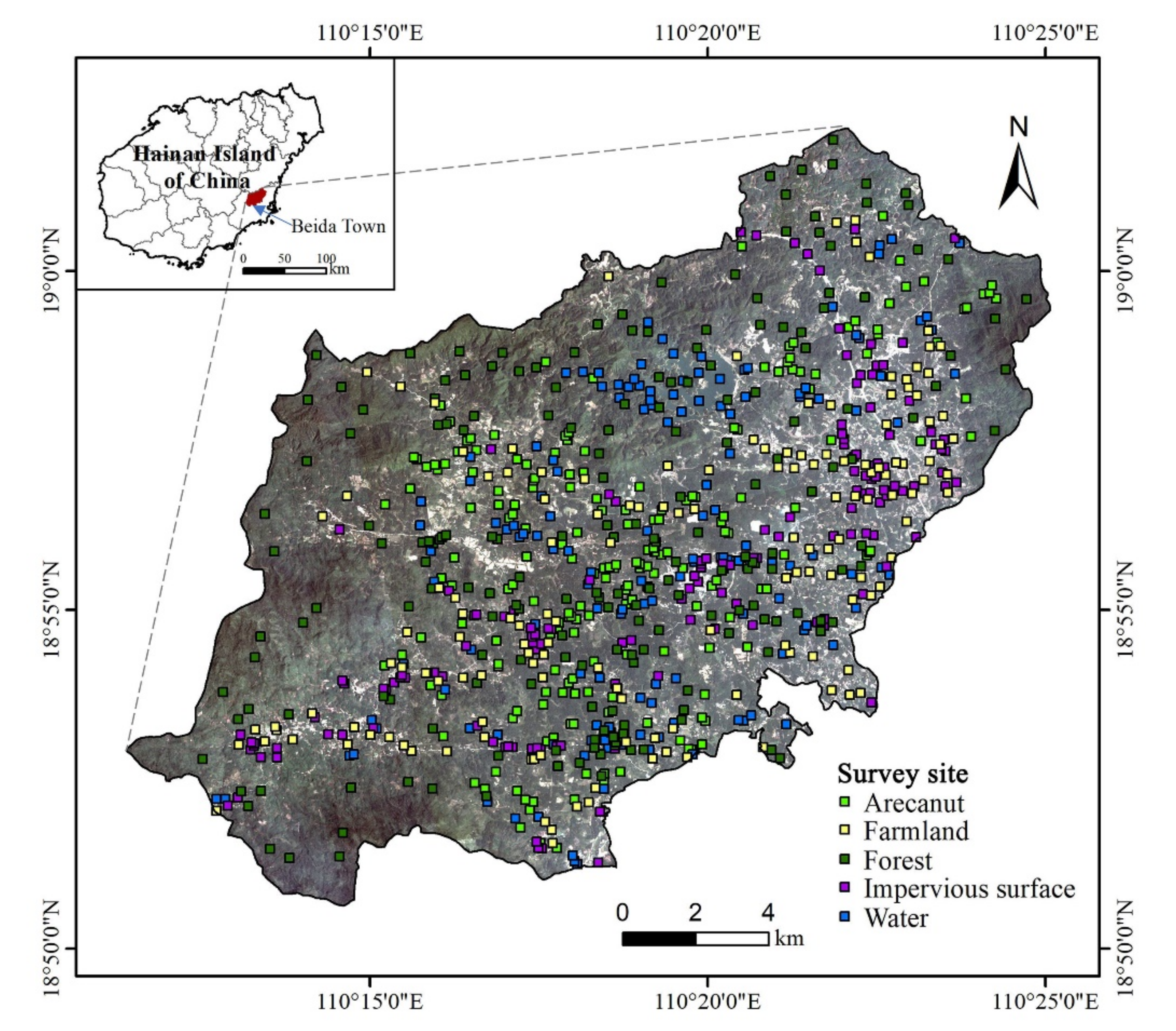
2.1. Study Area

The study area is located in Beida Town, Wanning City, Hainan Province, China (110°23′–110°40′ E, 18°86′–19°01′ N) with an area of 276.09 km2 (Figure 1). The area has a tropical monsoon climate, with an average annual temperature of 23.6 °C, a monthly average temperature of 18.7–28.5 °C, annual precipitation of approximately 2200 cm, and average annual sunshine hours over 1800. Beida Town is located in a hilly mountainous area. The soil type is Ferralsols according to IUSS Working Group WRB [14].
Hainan Province contains the largest arecanut production area in China, with the greatest planting area located in Wanning City. In 2018, the planting area reached 18,138 hm2, accounting for 16.5% of the total planting area in Hainan [2]. Beida Town is the principal planting area of arecanut in Wanning City. The town also grows cash crops such as rubber, pineapple, and lychee.

2.2. Data Acquisition and Processing

2.2.1. PlanetScope Satellite Image Acquisition and Preprocessing

The PlanetScope small satellite constellation currently has more than 170 satellites in orbit, surpassing all current satellites in terms of resolution (3–4 m), frequency (daily), and global coverage [15]. In the current paper, we selected a high-quality clear and cloudless PlanetScope satellite image collected on 21 March 2019. The PlanetScope image used is an orthographic data product (3B) that has undergone sensor and radiometric calibration, as well as orthorectification and atmospheric correction. The satellite image has a spatial resolution of 3 m and contains four spectral bands in the blue, green, red, and near-infrared regions. Table 1 lists the PlanetScope satellite parameters.

2.2.2. Ground Sample Data Collection

The principal land use/cover types in the study area are farmland, forest, impervious surface (urban and rural areas; industrial and mining, water conservancy construction, and transportation land), water (rivers, lakes, ponds, etc.), and arecanut grove. Table 2 lists the visual interpretation characteristics of the main features in the study area. Ground sample data were obtained through field surveys with a GPS receiver on 19–21 March 2019. The coverage size of the field should be more than 10 m × 10 m. According to the location of the survey sites, the field boundaries were then drawn based on Google Earth Pro (version 7.3.2.5776). Finally, a total of 850 field polygon samples were determined. There are 150 samples for water, 150 for impervious surface, 200 for forest, 150 for farmland, and 200 for arecanut grove, with 70% and 30% of the samples used for training and verification, respectively.

2.3. Feature Variable Selection

2.3.1. Primary Selection of Characteristic Variables

  • Primary selection of spectral characteristic variables
The spectral characteristic variables initially selected included four original spectral bands and five widely used vegetation indices (Table 3). A spectral band can act as an important indicator for the extraction of ground feature information from remote sensing images. Here, we used the blue, green, red, and near-infrared reflectance bands of the PlanetScope image as the primary selection variables for spectral features. The blue band is susceptible to factors such as soil background, and plays a key role in the distinction between soil and vegetation; the green band is more sensitive to different types of plants and can be used to distinguish between vegetation types [16]; the red band is the principal absorption band of chlorophyll and is an important indicator of plant vitality [17]; and the near-infrared band can remove the influence of the atmosphere (e.g., aerosols and thin clouds) and can reflect the vegetation growth and coverage [18].
Based on the principal feature types in the study area, the Difference Vegetation Index (DVI), Modified Soil Adjusted Vegetation Index (MSAVI), Normalized Difference Vegetation Index (NDVI), Ratio Vegetation Index (RVI), and Soil Brightness Index (SBI) were selected (Table 3). DVI is extremely sensitive to changes in the soil background and can better identify vegetation and water bodies [19]; MSAVI can reflect the soil and vegetation coverage information on the ground under the influence of soil background factors, and can accurately identify low vegetation coverage [20]; NDVI is sensitive to green vegetation and can reflect vegetation growth status and coverage [21]; RVI enhances the radiation difference between vegetation and soil, and can characterize biomass information under different vegetation coverage [22]; and SBI is sensitive to the soil background and can effectively extract construction and bare land in the absence of vegetation cover [23].
  • Primary selection of texture feature variables
Texture is a visual feature that reflects the homogeneity of the image and describes the grayscale spatial distribution of the image pixel neighborhood [24]. Each feature contained in remote sensing images has its own unique texture structure. However, the spectrum of an object may vary between features, while different objects may also have the same spectrum, resulting in difficulties in identifying objects. The stem of the arecanut tree is upright, arborous, up to 30 m tall, and with obvious circular leaf marks. Moreover, the leaves are clustered at the top of the stem and with a length of 1.3–2 m. The tree bears fruit to many pines of a long and narrow lanceolate shape, a 30–60 cm length, and 2.5–4 cm width. The upper pinna is connate and the tip has irregular teeth. Furthermore, the arecanut has a row spacing of 2.5 to 3.0 m and a plant spacing of 2.0 to 2.5 m. Thus, the forests of this crop present textural features that are obviously distinct from other ground objects within the high spatial resolution remote sensing image.
We selected the Gray-Level Co-Occurrence Matrix (GLCM) method to select eight texture feature indicators: Mean (Me), Variance (Var), Homogeneity (Hom), Contrast (Con), Dissimilarity (Dis), Entropy (Ent), Second moment (SM), and Correlation (Cor), Table 4 shows their formulas [25]. Based on the four spectral bands of the PlanetScope satellite image, a total of 32 texture features were subsequently extracted.

2.3.2. Feature Variable Optimization Method

The random forest (RF) algorithm, proposed by Breiman and AdeleCulter in 2001, integrates multiple trees based on ensemble learning, with a single decision tree taken as the basic unit [26,27]. Due to its strong noise tolerance, avoidance of overfitting, and ability to handle high-dimensional data, RF is not only applied to classification tasks, but can also calculate the importance of a single feature variable. In particular, RF performs feature screening using a feature importance evaluation, whereby the contribution value of each feature on each decision tree is determined, and the average values are compared between features. The out-of-bag (OOB) error rate is typically used as the evaluation index to measure the feature contribution, denoting the variable importance (VI) of different feature variables. The feature optimization is then realized by ranking features by importance. The feature variable importance, VI, is calculated as follows:
V I = k = 1 N B n k M B o k M M
where N is the number of generated decision trees, M is the number of feature variables, B n k M is the out-of-bag error of the k-th decision tree when feature M is added to the noise interference, and B o k M is the out-of-bag error of the k-th decision tree without noise interference. The addition of feature M with random noise dramatically reduces the accuracy rate of the out-of-bag data, indicating the strong influence of this feature on the prediction results of the sample, and thus its importance is relatively high [28].

2.4. Classification Model Building Method

The proposed classification framework initially calculates the training sample feature variables and subsequently constructs three classification models based on the BP neural network (BPNN), RF, and support vector machine (SVM) algorithms. These models are applied to extract the arecanut and other surrounding ground features. The extraction results are then verified using the verification samples and compared to determine the most accurate classification model.

2.4.1. BP Neural Network Algorithm

BPNN is a multilayer feedforward neural network that adopts the error back propagation algorithm to train the model. As the most widely used neural network to date [29], it uses the gradient descent method to minimize the mean square error between the actual and expected output values. BPNN is able to perform both signal forward propagation and error backward propagation. The input signal of BPNN propagates forward through the input layer and each hidden layer, and finally reaches the output layer, where the actual output value is obtained and compared with the expected output value. If the two output values are not equal, the error will enter back propagation, where the output error is adjusted with a threshold and weight at each layer via gradient descent. This results in a neural network model that has an expected output value within the error tolerance range. The BPNN is composed of the input, output, and hidden layers, and is trained by constantly adjusting the threshold and weight. The specific implementation process is as follows:
  • Dataset entry: define randomly divided training set P_train, validation set T_test, training label P class and verification label T class.
  • Data normalization: the mapminmax function is used to normalize and map the data to the range of 0–1 to avoid significant differences between the input and output data.
  • A neural network is established and the network parameters are set.
  • The training parameters are defined and network training is performed. The number of iterations, learning rate, training error target, and maximum number of failures are set to 200, 0.001, 0.0001, and 10, respectively. The train (net, P, T) function is used for network training.
  • Network simulation is performed using the sim (net, test matrix) function and the overall recognition accuracy of BPNN is obtained based on the predicted and expected values.

2.4.2. Random Forest Algorithm

The application of RF in classification tasks centers around the bootstrap method to randomly extract and return s samples from the sample set. Following n sample iterations, n training sets are obtained with n decision tree models. The generated n decision trees are then integrated into a random forest with multiple tree classifiers to determine the final prediction result [28]. Multiple decision trees are constructed during the training phase and the final class output is the pattern of a single decision tree class. The number of decision trees ntree is set to 500, while all other parameters are taken as the default values.

2.4.3. Support Vector Machine

SVM, first proposed by Vapnik [30], is based on statistical learning theory, and in particular, the principle of structural risk minimization [31]. Under linear separability, SVM aims to determine the optimal classification hyperplane of the two types of samples in the original space. For linear inseparability, the relaxation variable is added for analysis, and the samples in the low dimensional input space are mapped to the high dimensional feature space via nonlinear mapping, resulting in linearity and allowing for the determination of the optimal hyperplane in the feature space. Optimizing the segmentation hyperplane separates the sample types and minimizes the error, resulting in the accurate classification of data. More details of the SVM calculation process can be found in the relevant literature [32]. SVM has a simple structure and strong adaptability and robustness, and is thus applicable to a wide range of linear, nonlinear, classification, and regression problems. We employed SVM to build a monitoring model for arecanut yellowing disease using the mapminmax function to normalize the training and validation sets and to scale the data within [0,1]. The svmtrain and svmpredict commands were then implemented in LIBSVM 3.23 to train the samples and test the validation set, respectively. SVM system default values were used for the linear kernel function and parameters such as penalty factor c and kernel parameter g.

3. Results

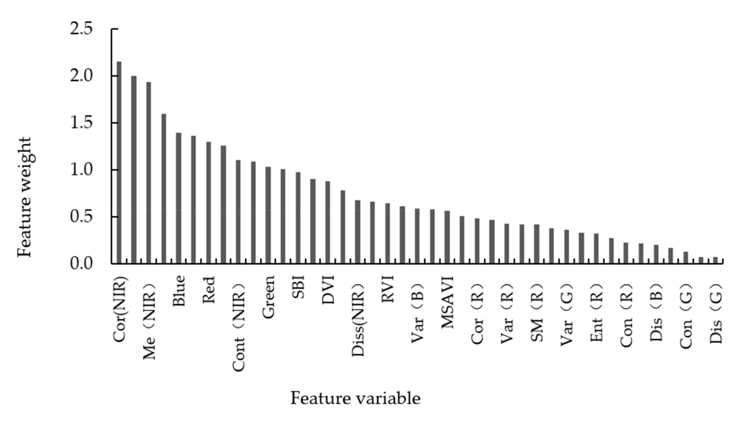
3.1. Feature Space Optimization

The initial feature space contains a total of 41 feature variables (9 spectral and 32 textural feature variables). A large number of feature variables will generate redundant data, increasing the model complexity and affecting the classification accuracy. We employed the RF algorithm to evaluate the importance of the 41 feature variables in the initial feature space, ranking their importance based on the feature variable weights. Figure 2 presents the importance rankings of the target feature variables, whereby the first 12 feature weights are greater than 1, the middle 12 feature weights range between 0.5 and 1, and the latter 17 feature weights are less than 0.5. Then, according to the order of feature importance, the first k (i = 1, 2, ……, 41) feature variables were selected to construct the random forest classification model of arecanut, and the overall classification accuracy was subsequently calculated. The overall classification accuracy is maximized to 88.3% when the number of feature variables equals 14. Therefore, the first 14 feature variables (CorNIR, VarNIR, MeNIR, MeR, RB, EntNIR, RR, RNIR, ConNIR, MeB, RG, NDVI, SBI, and HomNIR) were selected to construct the optimized feature space.

3.2. Extraction of Arecanut Planting Information

In this study, two feature spaces (i.e., initial feature space and optimized feature space) were used as the input of three machine learning algorithms (i.e., SVM, BPNN, and RF) to extract the arecanut planting information, respectively. A total of six classification models were constructed based on SVM, BPNN, and RF to extract the arecanut planting area in the study region, denoted as SVM-1, BPNN-1, and RF-1 for the initial feature space input and SVM-2, BPNN-2, and RF-2 for the optimized feature space as input. Ground survey data were used to evaluate the classification accuracy of the initial and optimized feature space inputs, and the impact of feature optimization on the extraction accuracy of arecanut planting area was then analyzed.
Table 5 reports the classification accuracy of arecanut based on the different classification models. Following RF feature optimization, the user’s and producer’s accuracy of SVM-2 are observed to exceed those of SVM-1 by 10.35% and 7.54%, respectively. The producer’s accuracy for BPNN-2 remained changed, while the user’s accuracy increased from 81.86% to 87.50%. In addition, the user’s and producer’s accuracy of the RF-2 model is 0.60% and 7.58% higher than those of the SVM-1 and RF-1 models, respectively. The overall accuracy of SVM-2, BPNN-2, and RF-2 is determined as 74.82%, 83.67%, and 88.30%, respectively, which is 3.90%, 7.77%, and 7.45% higher than that of SVM-1, BPNN-1, and RF-1. Moreover, the Kappa coefficients of SVM-2, BPNN-2, and RF-2 are 0.680, 0.795, and 0.853, respectively, exceeding those of SVM-1, BPNN-1, and RF-1.
In order to compare the extraction effects of SVM, BPNN, and RF on the arecanut planting area, we further compared and analyzed the classification results of SVM-2, BPNN-2, and RF-2 following feature space optimization (Table 5). RF-2 is observed to have the highest overall accuracy, improving on those of BPNN-2 and SVM-2 by 5.53% and 18.02%, respectively. In summary, the classification model following feature space optimization has the ability to improve the extraction accuracy of the arecanut planting area, with the feature optimized RF-2 model identified as the most suitable for arecanut planting information extraction, effectively improving the extraction accuracy of arecanut.
In order to verify the influence of different classification algorithms on the extraction accuracy of arecanut, we further constructed a confusion matrix for the classification results of SVM-2, BPNN-2, and RF-2 (Table 6) and investigated the omission and misclassification of arecanut. The SVM-2 results reveal that 17.19% of the identified arecanut are misclassified forest land and farmland, while 19.70% are misclassified as forest land. The BPNN-2 and RF-2 models reduced the omission and commission errors of arecanut compared to SVM-2, with RF-2 exhibiting the lowest omission and commission errors. Thus, the optimized RF-2 model is identified to have the greatest separability for arecanut, forest, and farmland.

3.3. Regional Application

In order to visually compare the classification effect of the study area images under different methods, we selected the central area of the study area image and employed SVM-2, BPNN-2, and RF-2 to determine the distribution map of the arecanut extraction results on a regional scale (Figure 3). Table 6 and Figure 3 reveal that the SVM-2 model has a serious leakage of cultivated land in the study area, almost all of which is classified as forest and arecanut. Furthermore, a large extent of forest is wrongly divided into arecanut. The BPNN model effectively overcomes the mixed separation of farmland and other vegetation, and the distinction between arecanut and forest is more obvious. The classification results of the RF model are generally consistent with those of the BPNN model, while the former improves on the misclassification of farmland in the northern region. In summary, based on the feature variables following RF feature optimization, the application of the RF method can extract the arecanut planting area in the study region more effectively compared to the BPNN and SVM models.
Arecanut planting area extraction models based on the support vector machine (SVM), BP neural network (BPNN), and random forest (RF) classification algorithms were then constructed. The overall classification accuracies of the SVM, BPNN, and RF models optimized by the RF features were determined as 74.82%, 83.67%, and 88.30%, with Kappa coefficients of 0.680, 0.795, and 0.853, respectively.

4. Discussion

The fusion of spectral and textural features to construct a classification model presented in the current paper has been demonstrated to achieve promising results in the extraction of arecanut planting area. However, numerous spectral features have not been considered. Follow-up research should include additional spectral features based on the extraction method of arecanut planting area employed in this paper. In addition, more data sources should be adopted to construct a more accurate method for the extraction of arecanut planting area.
The selection of characteristic variables is crucial for the construction of a classification model. In particular, the presence of irrelevant, weakly related, or redundant features in the primary selected features will directly affect the classification accuracy and generalization ability of the model [33]. Therefore, feature selection is required to remove such features. The RF feature variable optimization algorithm can determine each feature variable weight, reducing the redundancy of the feature variables and improving the classification accuracy and generalization ability. However, this optimization approach does not consider the correlation between various features, thus further improvement is required. Future research will focus on determining the feature correlations while removing the redundancy between the features. In addition, simpler and more efficient feature selection algorithms are required for the model input selection.
The choice of modeling method affects the accuracy of the classification model. Although SVM, BPNN, and RF have strong applications in research, they are associated with several limitations. For example, although the SVM method is able to deal with various nonlinear problems through the selection of the kernel function, determining the kernel function and related parameters proves to be a difficult task, thus restricting its application [34]. The work presented in the current paper is not based on certain theoretical standards and only the linear kernel function is selected. The next step should consider other kernel functions in order to select the optimal function, which can then allow for the further optimization of the model parameters to obtain a higher precision model. The BPNN method has strong nonlinear fitting and generalization abilities, and the established network model is stable. However, the BPNN method also faces limitations, for example, the accurate determination of the number of hidden layer nodes. In particular, the network fails to converge for small node numbers and the fault tolerance is poor, while for a large number of nodes, the network has a long learning time and is prone to overfitting. Although RF has a strong tolerance to noise and is not prone to overfitting, its parameters are more complicated and features with more value divisions are likely to have a greater impact on RF decision-making, thereby affecting the accuracy of the model. Determining how to improve these methods is reserved for future work.

5. Conclusions

Current methods based on low- and medium-resolution satellite images are not able to meet the demand for the high-precision extraction of arecanut area in Hainan due to the cloudy and rainy climate and severe land fragmentation. In the current paper, a high-precision extraction method for arecanut planting area was proposed based on image feature space optimization using PlanetScope satellite imagery. Results demonstrate the ability of the spectral and texture features of PlanetScope satellite data to effectively extract the planting distribution of arecanut. The Kappa coefficients of the SVM, BPNN, and RF models following the RF feature optimization were determined as 0.680, 0.795, and 0.853, with overall classification accuracies of 74.82%, 83.67%, and 88.30%, respectively. The application of feature optimization improves the overall accuracy by 3.90%, 7.77% and 7.45%, respectively. This indicates the strong applicability of feature space optimization based on PlanetScope satellite imagery for the extraction of arecanut planting area. The research results provide theoretical and technical references for the remote sensing extraction of agricultural and forestry information.

Author Contributions

Conceptualization, information analysis, and writing of original draft, Y.J. and J.G.; methodology, W.H. and J.Z.; software, B.C.; investigation, writing—review and editing and funding acquisition, H.Y. All authors have read and agreed to the published version of the manuscript.

Funding

This research was funded by Hainan Provincial Major Science and Technology Program of China (ZDKJ2019006); Youth Innovation Promotion Association CAS (2021119); Future Star Talent Program of Aerospace Information Research Institute, Chinese Academy of Sciences (2020KTYWLZX08); National special support program for high-level personnel recruitment (Wenjiang Huang).

Institutional Review Board Statement

Not applicable.

Informed Consent Statement

Not applicable.

Data Availability Statement

The data are available from the corresponding author, at reasonable request.

Conflicts of Interest

The authors declare no conflict of interest.

References

  1. Graham, P. Traditional medical treatments III: Betel nut (Areca catechu). Ann. ACTM Int. J. Trop. Travel Med. 2005, 6, 13–14. [Google Scholar] [CrossRef]
  2. Hainan Provincial Bureau of Statistics, Survey Office of National Bureau of Statistics in Hainan. Hainan Statistical Yearbook 2020; China Statistical Publishing House: Beijing, China, 2020. (In Chinese)
  3. Sun, H.; Gong, M. Current development status and countermeasures of arecanut planting and processing industry in Hainan. Chin. J. Trop. Agric. 2019, 39, 91–94, (In Chinese with English abstract). [Google Scholar] [CrossRef]
  4. Noguchi, N.; O’Brien, J.G. Remote sensing technology for precision agriculture. Environ. Control Biol. 2003, 41, 107–120. [Google Scholar] [CrossRef]
  5. Hayes, M.J.; Decker, W.L. Using satellite and real-time weather data to predict maize production. Int. J. Biometeorol. 1998, 42, 10–15. [Google Scholar] [CrossRef]
  6. Onojeghuo, A.O.; Blackburna, G.A.; Huang, J.; Kindredc, D.; Huang, W. Applications of satellite ‘hyper-sensing’ in Chinese agriculture: Challenges and opportunities. Int. J. Appl. Earth Obs. Geoinf. 2018, 64, 62–86. [Google Scholar] [CrossRef] [Green Version]
  7. Zheng, H.; Zhou, X.; He, J.; Yao, X.; Tian, Y. Early season detection of rice plants using rgb, nir-g-b and multispectral images from unmanned aerial vehicle (UAV). Comput. Electron. Agric. 2020, 169, 105223. [Google Scholar] [CrossRef]
  8. Shen, K.; Li, W.; Pei, Z.; Fei, W.; Sun, G.; Zhang, X.; Chen, X.; Ma, S. Crop area estimation from UAV transect and MSR image data using spatial sampling method. Procedia Environ. Sci. 2015, 26, 95–100. [Google Scholar] [CrossRef] [Green Version]
  9. Fu, Z.; Jiang, J.; Gao, Y.; Krienke, B.; Liu, X. Wheat growth monitoring and yield estimation based on multi-rotor unmanned aerial vehicle. Remote Sens. 2020, 12, 508. [Google Scholar] [CrossRef] [Green Version]
  10. Ládai, A.D.; Barsi, Á. Analysing automatic satellite image classification in the desert of Sudan. Period. Polytech. Civ. Eng. 2008, 52, 23–27. [Google Scholar] [CrossRef]
  11. Pan, Y.; Li, L.; Zhang, J.; Liang, S.; Zhu, X.; Sulla-Menashe, D. Winter wheat area estimation from modis-evi time series data using the crop proportion phenology index. Remote Sens. Environ. 2012, 119, 232–242. [Google Scholar] [CrossRef]
  12. Zhang, M.; Lin, H. Object-based rice mapping using time-series and phenological data. Adv. Space Res. 2019, 63, 190–202. [Google Scholar] [CrossRef]
  13. Liu, J.; Tian, Q.; Huang, Y.; Du, L.; Wang, L. Extraction of the corn planting area based on multi-temporal HJ-1 satellite data. In Proceedings of the 19th International Conference on Geoinformatics, Shanghai, China, 24–26 June 2011; IEEE: Piscataway, NJ, USA, 2011. [Google Scholar] [CrossRef]
  14. IUSS Working Group WRB. World Reference Base for Soil Resources 2006; World Soil Resources Reports No. 103; FAO: Rome, Italy, 2006. [Google Scholar]
  15. Planet Team. Planet Application Program Interface: In Space for Life on Earth; Planet Labs Inc.: San Francisco, CA, USA, 2018; Available online: https://api.planet.com (accessed on 2 March 2018).
  16. Huang, Z.; Cao, C.; Chen, W.; Xu, M.; Dang, Y.; Singh, R.P.; Bashir, B.; Xie, B.; Lin, X. Remote sensing monitoring of vegetation dynamic changes after fire in the Greater Hinggan Mountain Area: The algorithm and application for eliminating phenological impacts. Remote Sens. 2020, 12, 156. [Google Scholar] [CrossRef] [Green Version]
  17. Zhang, J.; Pu, R.; Yuan, L.; Huang, W.; Nie, C.; Yang, G. Integrating remotely sensed and meteorological observations to forecast wheat powdery mildew at a regional scale. IEEE J. Sel. Top. Appl. Earth Observ. Remote Sens. 2017, 7, 4328–4339. [Google Scholar] [CrossRef]
  18. Zeng, C.; Binding, C. The effect of mineral sediments on satellite chlorophyll-a retrievals from line-height algorithms using red and near-infrared bands. Remote Sens. 2019, 11, 2306. [Google Scholar] [CrossRef] [Green Version]
  19. Jordan, C.F. Derivation of leaf area index from quality of light on the forest floor. Ecology 1969, 50, 663–666. [Google Scholar] [CrossRef]
  20. Qi, J.; Chehbouni, A.; Huete, A.R.; Kerr, Y.H.; Sorooshian, S. A modified soil adjusted vegetation index. Remote Sens. Environ. 1994, 48, 119–126. [Google Scholar] [CrossRef]
  21. Rouse, J.W.; Haas, R.H.; Deering, D.W.; Schell, J.A. Monitoring the Vernal Advancement of Retrogradation of Natural Vegetation; NASA/GSFC, Type III, Final Report; NASA/GSFC: Greenbelt, MD, USA, 1974. Available online: https://ntrs.nasa.gov/api/citations/19740004927/downloads/19740004927.pdf (accessed on 20 December 2020).
  22. Huete, A.R.; Jackson, R.D. Suitability of spectral indices for evaluating vegetation characteristics on arid rangelands. Remote Sens. Environ. 1987, 23, 213–232. [Google Scholar] [CrossRef]
  23. Ren, C. Study on Extraction of Mango Forest with High Resolution Remote Sensing Image; Institute of Remote Sensing and Digital Earth, Chinese Academic of Sciences: Beijing, China, 2017; (In Chinese with English abstract). [Google Scholar]
  24. Soares, J.V.; Rennó, C.D.; Formaggio, A.R.; Yanasse, C.C.F.; CesarFrery, A. An investigation of the selection of texture features for crop discrimination using SAR imagery. Remote Sens. Environ. 1997, 59, 234–247. [Google Scholar] [CrossRef]
  25. Haralick, R.M.; Shanmugam, K.; Dinstein, I. Textural features for image classification. Stud. Media Commun. 1973, 3, 610–621. [Google Scholar] [CrossRef] [Green Version]
  26. Kwok, S.W.; Carter, C. Multiple decision trees. Mach. Intell. 2013, 9, 327–335. [Google Scholar] [CrossRef]
  27. Pavlov, Y.L. Limit distributions of the height of a random forest. Theor. Probab. Appl. 2006, 28, 471–480. [Google Scholar] [CrossRef]
  28. Rodriguez-Galiano, V.F.; Chica-Olmo, M.; Abarca-Hernandez, F.; Atkinson, P.M.; Jeganathan, C. Random forest classification of mediterranean land cover using multi-seasonal imagery and multi-seasonal texture. Remote Sens. Environ. 2012, 121, 93–107. [Google Scholar] [CrossRef]
  29. Wang, S.; Zhang, N.; Wu, L.; Wang, Y. Wind speed forecasting based on the hybrid ensemble empirical mode decomposition and GA-BP neural network method. Renew. Energy 2016, 94, 629–636. [Google Scholar] [CrossRef]
  30. Mavroforakis, M.E.; Theodoridis, S. A geometric approach to support vector machine (SVM) classification. IEEE Trans. Neural Networks 2006, 17, 671–682. [Google Scholar] [CrossRef] [PubMed]
  31. Lesser, B.; Mücke, M.; Gansterer, W.N. Effects of reduced precision on floating-point SVM classification accuracy. Procedia Comput. Sci. 2011, 4, 508–517. [Google Scholar] [CrossRef] [Green Version]
  32. He, Q.; Xie, Z.; Hu, Q.; Wu, C. Neighborhood based sample and feature selection for SVM classification learning. Neurocomputing 2011, 74, 1585–1594. [Google Scholar] [CrossRef]
  33. Dash, M.; Liu, H. Feature selection for classification. Intell. Data Anal. 1997, 1, 131–156. [Google Scholar] [CrossRef]
  34. Wang, L.; Zhang, S. Incorporation of texture information in a SVM method for classifying salt cedar in western China. Remote Sens. Lett. 2014, 5, 501–510. [Google Scholar] [CrossRef]
Figure 1. Geographic location of the study area with the spatial distribution of land use/cover type survey sites.
Agriculture 11 00371 g001
Figure 2. Importance ranking of the first 14 feature variables for constructing the optimized feature space.
Agriculture 11 00371 g002
Figure 3. The distribution map of arecanut extracted based on different classification models with the feature space optimization of PlanetScope imagery. (a) SVM-2, (b) BPNN-2, and (c) RF-2.
Agriculture 11 00371 g003
Table 1. Specifications of PlanetScope satellite.
ParameterParameter Value
TrackInternational Space Station OrbitSun-synchronous orbit
Orbital inclination52°, 98°
Spatial resolution3–4 m
Spectral bandBand1: Blue (455–515 nm)
Band2: Green (500–590 nm)
Band3: Red (590–670 nm)
Band4: NIR (780–860 nm)
Track height400 km, 475 km
Sensor typeBayer filter CCD camera
Width24.6 km × 16.4 km
Table 2. Visual interpretation signs of features in the study area.
Feature CategoryImage CharacteristicsFeature Description
Water Agriculture 11 00371 i001Light green, the larger the water body, the darker the color. Pit ponds are small in area, with clear boundaries and irregular shapes; rivers are in regular curved strips; lakes have large water areas, darker colors, and irregular shapes.
Impervious surface Agriculture 11 00371 i002Light purple and brown with irregular shapes, bare soil, and less vegetation coverage.
Forest Agriculture 11 00371 i003Dark green, the plots are irregularly distributed, with uniform tone and clear texture.
Farmland Agriculture 11 00371 i004Light green, with clear stripes, regular continuous distribution, and uniform texture.
Arecanut Agriculture 11 00371 i005Light green, granular canopy distributed in a large area, irregular plot shape, uniform texture, and small amount of soil exposure.
Table 3. Description of the spectral characteristic variables selected in this study.
Spectral CharacteristicFormula 1Reference
Blue bandRB[16]
Green bandRG[16]
Red bandRR[17]
Near-infrared bandRNIR[18]
Difference Vegetation Index (DVI) R N I R R R [19]
Modified Soil Adjusted Vegetation Index (MSAVI) 1 2 [ 2 R N I R + 1 2 R N I R + 1 2 8 R N I R R R ] [20]
Normalized Difference Vegetation Index (NDVI) ( R N I R R R ) / ( R N I R + R R ) [21]
Ratio Vegetation Index (RVI) R N I R / R R [22]
Soil Brightness Index (SBI) R N I R 2 + R R 2 [23]
1RR, RG, RB, and RNIR denote the red, green, blue, and near-infrared band.
Table 4. Description of the texture features selected in this study.
Texture FeatureFormula 1Description
Mean i j P i , j × i Reflects the regular degree of texture.
Variance i j i M e a n 2 × P i , j Reflects the deviation between the pixel and mean values; the larger the grayscale change, the larger the value.
Homogeneity i j P i , j × 1 1 + i j 2 Reflects the local gray uniformity of the image; the more uniform the local, the larger the value.
Contrast i j P i , j × i j 2 Reflects the sharpness of the image and the depth of the texture.
Dissimilarity i j P i , j × i j Similar to contrast, with greater linearity; the higher the local contrast, the higher the dissimilarity.
Entropy i j P i , j × l o g   P i , j Reflects the texture complexity; the larger the value, the more complex the texture.
Second Moment i j P i , j 2 Reflects the uniformity of the image distribution and texture thickness.
Correlation i j i M e a n × j M e a n × P i , j 2 V a r i a n c e Reflects the image local relevance.
1P(i, j) is the element value of the image at point (i, j).
Table 5. The classification accuracy of arecanut based on different classification models with different feature subsets.
ModelOmission Error/%Commission Error/%User’s Accuracy/%Producer’s Accuracy/%Overall Accuracy/%Kappa Coefficient
SVM-124.2427.5472.4675.7670.920.630
BPNN-115.1518.8481.1684.8575.900.698
RF-113.648.0691.9486.3680.850.760
SVM-219.7017.1982.8183.3074.820.680
BPNN-215.1512.5087.5084.8583.670.795
RF-26.067.4692.5493.9488.300.853
Table 6. Confusion matrix of the classification results based on SVM-2, BPNN-2 and RF-2 models.
Model.Land Use TypeWaterImpervious SurfaceForestFarmlandArecanutTotal
SVM-2Water49000049
Impervious surface05000050
Forest10594613119
Farmland000000
Arecanut00745364
Total5050665066282
BPNN-2Water49000049
Impervious surface05000050
Forest005015469
Farmland101231650
Arecanut00445664
Total5050665066282
RF-2Water49000049
Impervious surface05000050
Forest005717175
Farmland10631341
Arecanut00326267
Total5050665066282
Publisher’s Note: MDPI stays neutral with regard to jurisdictional claims in published maps and institutional affiliations.

