
Classification of Amanita Species Based on Bilinear Networks with Attention Mechanism

College of Mechanical and Electrical Engineering, Sichuan Agricultural University, Ya’an 625000, China
*
Author to whom correspondence should be addressed.
Agriculture 2021, 11(5), 393; https://0-doi-org.brum.beds.ac.uk/10.3390/agriculture11050393
Submission received: 8 April 2021
/
Revised: 20 April 2021
/
Accepted: 22 April 2021
/
Published: 26 April 2021
(This article belongs to the Special Issue Image Analysis Techniques in Agriculture)
Abstract
:The accurate classification of Amanita is helpful to its research on biological control and medical value, and it can also prevent mushroom poisoning incidents. In this paper, we constructed the Bilinear convolutional neural networks (B-CNN) with attention mechanism model based on transfer learning to realize the classification of Amanita. When the model is trained, the weight on ImageNet is used for pre-training, and the Adam optimizer is used to update network parameters. In the test process, images of Amanita at different growth stages were used to further test the generalization ability of the model. After comparing our model with other models, the results show that our model greatly reduces the number of parameters while achieving high accuracy (95.2%) and has good generalization ability. It is an efficient classification model, which provides a new option for mushroom classification in areas with limited computing resources.
1. Introduction
Amanita is a large fungus, which is an important part of natural medicine resources. At present, using the characteristics of amatoxins to control and treat tumors is a promising method [1,2,3]. Amanita muscaria is a famous hallucinogenic mushroom, which can be used to develop special drugs for anesthesia and sedation [4]. In terms of biological control, the toxins contained in Amanita albicans and Amanita muscaria have certain trapping and killing effects on insects or agricultural pests [3,5]. At present, there is no artificially cultivated Amanita, the amatoxins needed in scientific research can only be extracted from fruit bodies collected in the field [6,7,8]. Moreover, due to the lack of knowledge and ability to identify poisonous mushrooms, there are a number of cases of poisoning death from eating wild mushrooms every year [9,10,11,12,13]. In Europe, 95% of mushroom poisoning deaths are caused by poisonous Amanita [14,15]. Therefore, it is necessary to accurately classify and identify them both in terms of use value and poisoning prevention.
Many researchers have contributed to the classification of mushrooms. For example, Ismail [16] studied the characteristics of mushrooms, such as the shape, surface and color of the cap, roots and stems, and used the principal component analysis (PCA) algorithm to select the best features for the classification experiment using the decision tree (DT) algorithm. Pranjal Maurya [17] used a support vector machine (SVM) classifier to distinguish edible and poisonous mushrooms, with an accuracy of 76.6%. Xiao [18] used the Shuf-fleNetV2 model to quickly identify the toxicity of wild bacteria. The accuracy of the model is 55.18% for Top-1 and 93.55% for Top-5. Chen [19] used the Keras platform to build a convolutional neural network (CNN) for end-to-end model training and migrated to the Android end to realize mushroom recognition on the mobile end, but the recognition effect of his model was poor. Preechasuk J [20] proposed a new model of classifying 45 types of mushrooms including edible and poisonous mushrooms by using a technique of CNN, which gives the results of 0.78, 0.73 and 0.74 of precision, recall and F1 score, respectively. Dong J [21] proposed a CNN model that can detect qualified and three common types of substandard enoki mushroom caps and achieved 98.35% accuracy. However, this model is suitable for few types of mushrooms, and the cap must be detected.
Since the method based on the visual attention mechanism [22,23] can locate the distinguishable areas in the image without additional annotation information, it has been widely used in the field of fine-grained classification of images in recent years. At present, the mainstream attention mechanism can be divided into the following three types: channel attention, spatial attention and self-attention.
Channel attention aims to show the correlation between different channels. In a convolutional neural network, each image is initially represented by three channels (R, G, B) [24]. After different convolution kernels are processed, each channel will generate a new channel with different information. Channel attention automatically obtains the importance of each feature channel through network learning, and finally assigns different weight coefficients to each channel. It can achieve the purpose of strengthening important channels and suppressing non-important channels.
Spatial Attention is designed to enhance the spatial characteristics of expression of critical areas. DeepMind designed a Spatial Transformer Layer (STL) to realize spatial invariance [25,26]. Its principle is to transform the spatial information in the original picture into another space and retain the key information through STL. Then, generate a weight mask for each position and weigh the output. This method can enhance the specific target area of interest while weakening the irrelevant background area to extract the key information.
Self-attention reduces the dependence on external information and uses the inherent information within the feature to interact with attention as much as possible [27,28]. However, the disadvantage of this method is that every point must capture global contextual information, which will cause a lot of computational complexity and memory capacity, and the information on the channel is not considered.
In this paper, a method of CNN combined with an attention mechanism is proposed to solve the problem of difficult classification and identification of Amanita. The specific contributions and innovations are as follows:
- (1)
- A self-built Amanita dataset that is 3219 Amanita images obtained from the Internet and divided.
- (2)
- The Bilinear convolutional neural networks model was built and fine-tuned to make the model more suitable for the dataset.
- (3)
- The Bilinear convolutional neural networks model is combined with the attention mechanism to improve the model. This method can quickly obtain the most effective information.
2. Materials and Methods
2.1. Image Dataset
In this paper, the original dataset comes from two sources. On the one hand, it is a downloaded mushroom dataset from the Kaggle platform. The data on Kaggle are a public data source and have a certain degree of authority. Special thanks are owed to the Nordic Society of Mycologists, who provided the most common mushroom sources in the region on Kaggle and checked the data and labels. We choose the Amanita dataset based on the label of the mushroom dataset. Another dataset of mushroom images was collected from http://www.mushroom.world (accessed on 24 September 2020). We searched the mushroom database on this website based on the name of the mushroom. Then, we recorded the color and structure of the cap of Amanita (such as egg-shaped, unfolded cap, umbrella-shaped, spherical) according to [29] to confirm the type of Amanita again. Finally, the dataset of Amanita was obtained, as shown in Table 1.
In the paper, in order to make the model more applicable to the wild environment, most of the data pictures are Amanita growing in the wild environment, but also include some pictures of Amanita that were picked by hand.
2.2. Data Augmentation
There are seven kinds of Amanita in the original dataset, a total of 3219 pictures. All samples are randomly divided into training and test dataset according to a ratio of 8:2.
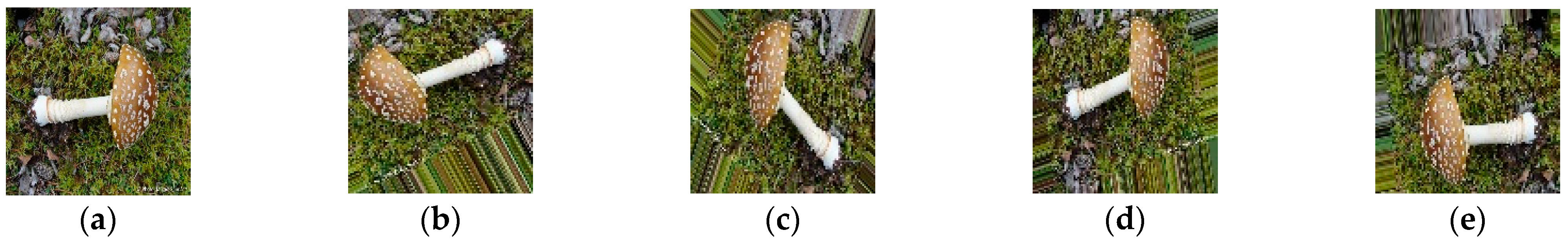
Training convolutional neural networks requires a lot of image data to prevent overfitting. Therefore, in this paper, the input image data are enhanced by using the built-in ImageDataGenerator [30,31] interface of Tensorflow2.0. The purpose of increasing the number of images is achieved by combining random rotation, translation, cutting and other operations, as shown in Figure 1b–e. This method roughly increases the number of images by 6 times.
2.3. Method
2.3.1. The Efficient Net Model
The Efficient Net [32] was proposed by the google team in 2019. Through comprehensive optimization of network width, depth, and input image resolution to achieve the goal of index improvement. It has fewer model parameters, but higher accuracy.
2.3.2. Bilinear Convolutional Neural Networks
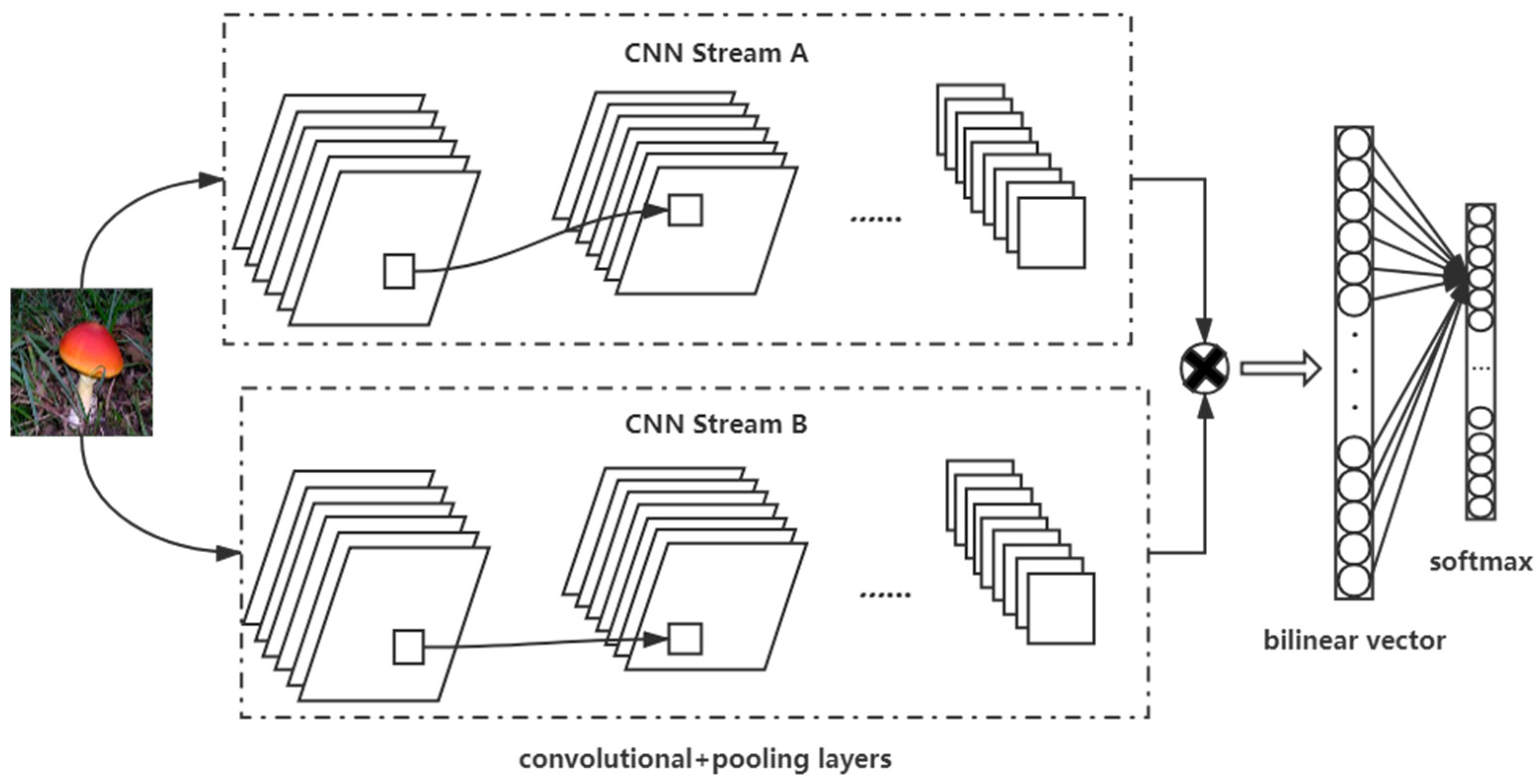
The Bilinear convolutional neural networks (B-CNN) [35,36] proposed by Lin in 2015 is a representative of weakly supervised fine-grained classification. Its network structure is shown in Figure 3. It used two A and B two-way convolutional neural networks to extract two features at each position of the image, then multiply the outer product, and finally classify through the classification layer.
The models are coordinated with each other through the CNN A and CNN B networks. The function of CNN A is to locate the feature parts of the image, and CNN B is used to extract the features of the feature regions detected by CNN A [37]. In this way, the local detection and feature extraction tasks in the fine-grained image classification process can be completed.
2.3.3. Visual Attention Mechanism
In this paper, we chose to use Mixed attention, which combines multiple attention mechanisms. It can bring better performance to a certain extent. An excellent work in this area is the Convolutional Attention Mechanism Module (CBAM) [38], which is based on the channel attention module (CAM) and connected with a spatial attention module (SAM). CAM and SAM are shown in Figure 4.
CAM uses the max-pooling output and the average-pooling output through the shared network [39]. SAM generates two feature maps representing different information by performing global average pooling and global maximum pooling operations. After merging the two feature maps, the feature fusion is performed through a 7 × 7 convolution with a larger receptive field, and finally the weight map is generated by the Sigmoid operation and superimposed back onto the original input feature map [40]. It achieves the purpose of enhancing the target area.
2.3.4. Our Model
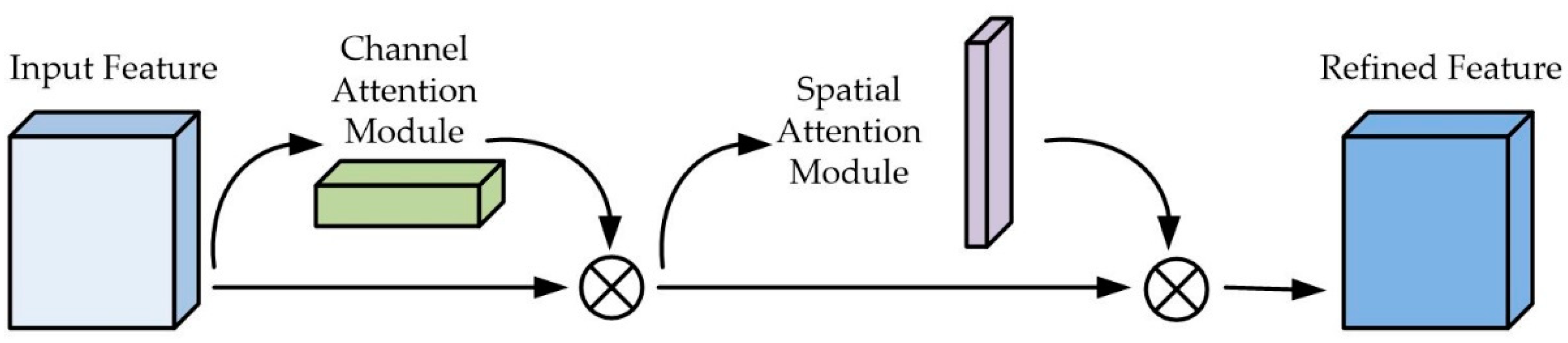
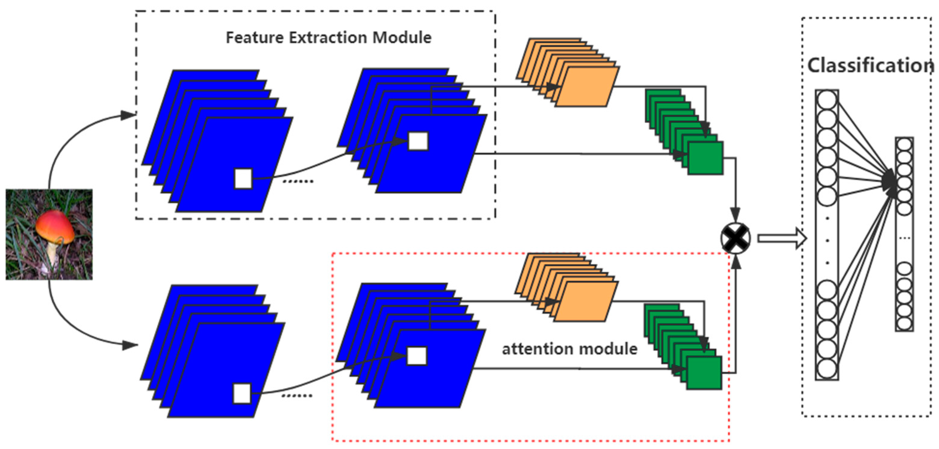
In this paper, a bilinear EfficientNet-B4 model is built and combined with the convolutional attention mechanism module (CBAM), CBAM as shown in Figure 5, which is a combination of spatial and channel modules. The structure of adding the attention mechanism to the bilinear model is shown in Figure 6.
The overall process of using the model is:
- (1)
- Use the EfficientNet-B4 network architecture to extract the feature layer after data expansion of the input image.
- (2)
- Combining the output result of the convolutional layer with CBAM, it will first pass a channel attention module to obtain the weighted result, then pass through a spatial attention module, and finally obtain the extracted result by weighting.
- (3)
- Multiply the extraction results obtained by CBAM with the feature layer one by one.
- (4)
- Join the fully connected layer for classification to obtain the final classification result.
2.4. Parameters and Index
In the choice of the optimizer, we compared the two optimizers stochastic gradient descent (SGD) [41] and adaptive moment estimation (Adam) [42], and found that the performance of the model decreased by about 1% when the SGD optimizer with a set learning rate of 0.001 and momentum of 0.95 was used, so we choose the Adam optimizer with hyperparameters beta_1 = 0.9, beta_2 = 0.999, epsilon =1 × 10⁻⁸, decay = 0.0 as the optimizer of models. In order to compare the accuracy and efficiency of different models, we used unified hyperparameters to train different network models (Table 2).
The simplest and most commonly used metric for evaluating classification models is accuracy, but precision and recall are also needed to evaluate the quality of the model. Precision [43] can be understood as the number of correctly predicted Amanita species images divided by the number of Amanita images predicted by the classifier. Recall [44] is the percentage of the number of correctly predicted Amanita species images to the total number of images actually belonging to the category of Amanita images. is the harmonic mean of precision and recall. Accuracy, Precision, Recall, and are defined as follows:
where TP and TN represent the Amanita image correctly classified; FP and FN indicate that the image of Amanita is misclassified.
3. Experimental Results and Discussion
3.1. Model Training
In this paper, the experimental environment is on the Google Colaboratory platform, which uses Tesla K80 GPU resources. The programming environment is Python3, and the framework structure is Keras 2.1.6 and Tensorflow 1.6.
The specific model training steps are as follows:
- Data loading;
A batch of Amanita pictures (32 pictures) were randomly loaded from the training dataset for subsequent data processing.
- Image preprocessing;
Preprocess the image to change the image size to 224 × 224 × 3. Then, put it through the Tensorflow2.0 built-in ImageDataGenerator for data enhancement.
- Define the model structure and load the pre-training weights;
Load the model (such as EfficientNet-B4) and fine-tune the model. Change the fully connected layer to a custom layer and modify the Softmax layer to seven layers according to the number of classifications required. In this paper, different layers are frozen according to the different models, and the method of transfer learning [45] is used to perform pre-training with Imagenet weights.
- Start training;
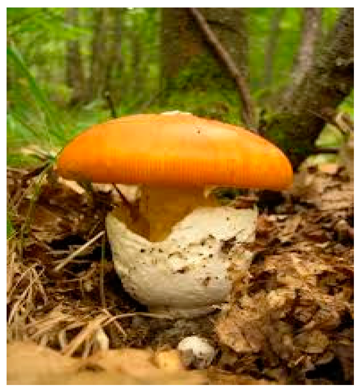
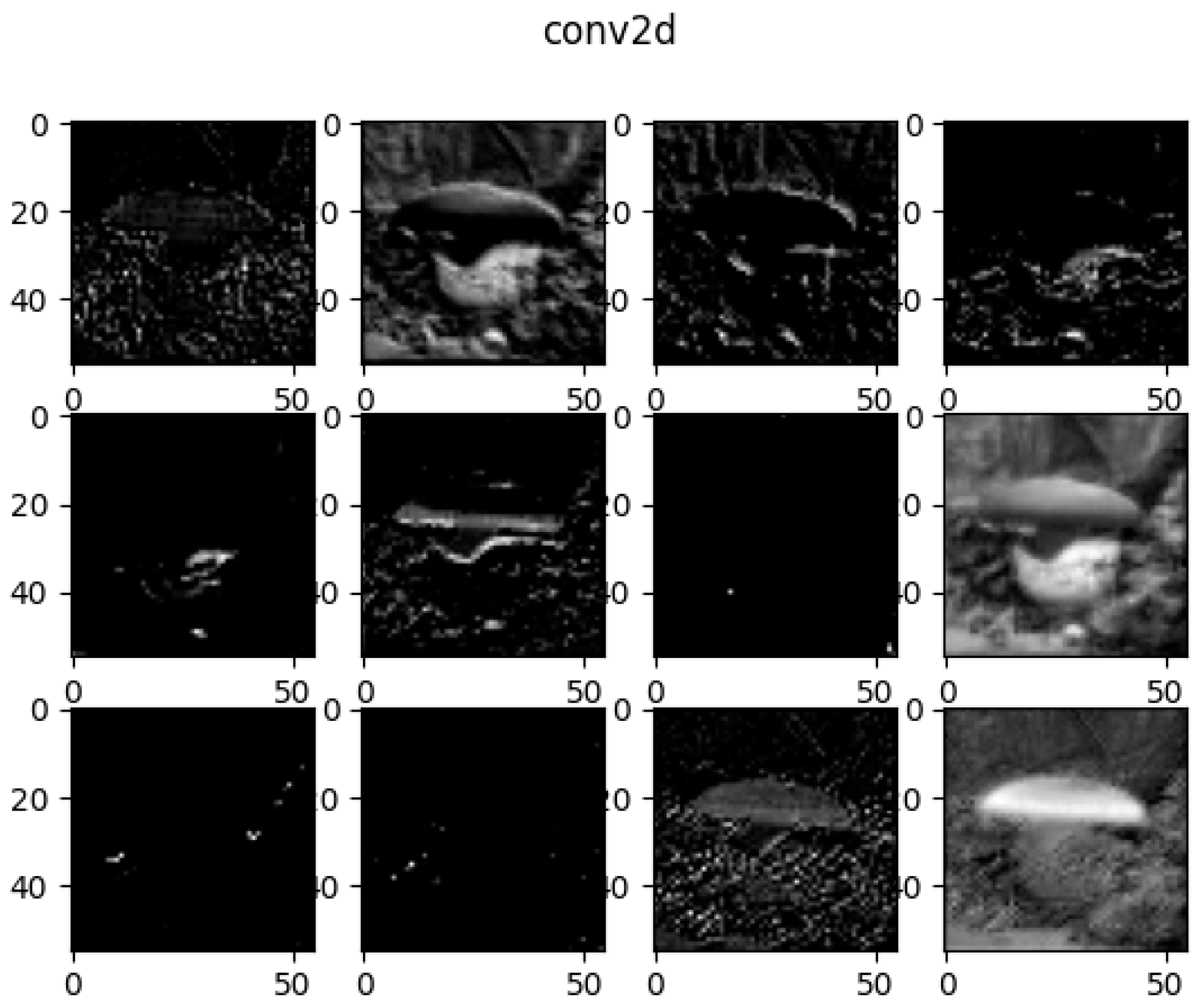
Before training the model, it is necessary to set the hyperparameters and optimizers related to the network structure. Pass the training dataset pictures (as shown in Figure 7) to the neural network for training. Among them, the feature map of the first convolutional layer (as shown in Figure 8), after one round of model training, obtains the loss and accuracy of the training dataset.
- Stop training;
This experiment is to avoid overtraining the network. An early stopping strategy is set, and the loss is verified by monitoring the training process. When the verification loss does not change within five rounds or the model training reaches the preset value, the model will stop training.
3.2. Comparison of Modeling Methods
In order to verify the performance of the model, we compared the proposed model with other CNN models on the dataset. The structure and parameters of these models are shown in Table 3.
In this paper, the steps of the comparison experiment are: (1) Use the VGGnet model with 16 layers (VGG-16) [46], the Residual Network with 50 layers (ResNet-50) [47], compare these two network models with EfficientNet-B4. (2) Combine the bilinear model to build a bilinear EfficientNet-B4, compare the bilinear VGG-16 model (B-CNN(VGG-16, VGG-16)) and the B-CNN(VGG-16, ResNet-50) model. (3) Add an attention mechanism to the model, conduct a comparative experiment, and discuss the effect of adding an attention mechanism.
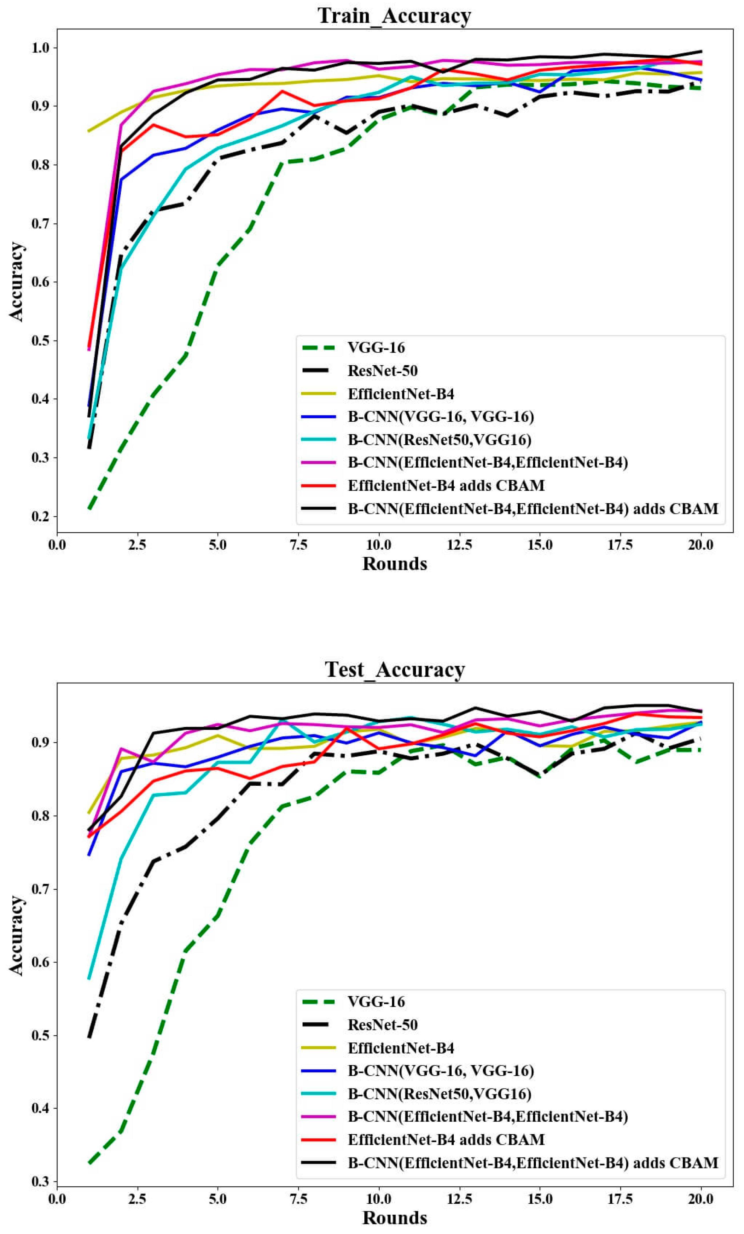
Figure 9 shows the changes in loss and accuracy during training and testing. Table 4 compares the results of different methods. The comprehensive chart can be used to draw the following conclusions:
- (1)
- The EfficientNet-B4 is superior to VGG-16 and Resnet-50 in terms of accuracy, model parameters and model size.
- (2)
- On this basis, the bilinear structure was studied and used, and it was found that B-CNN(VGG-16, ResNet-50) has good accuracy. However, it has the largest number of parameters in the model used, and the size of the model is also very large. However, Bilinear EfficientNet-B4 has a good performance in accuracy, model size and number of parameters.
- (3)
- For EfficientNet-B4 (accuracy rate is 92.76%), after adding the attention mechanism, its accuracy rate is 93.53%, which improves the accuracy rate by 0.77%; after combining the bilinear structure and attention mechanism, its accuracy rate is 95.2%, an increase of 1.77%. In general, adding an attention mechanism to the model will increase the accuracy by about 1% and can reduce the time by 0.5 s.
In addition, by comparing the first five rounds of training and testing in Figure 9, it can be found that the accuracy of the test is slightly higher than that of the training. The main reason is that the network is initialized with pre-trained weights. Therefore, the model has better feature extraction capabilities in the first few rounds of testing.
3.3. Model Test Results
Not all objects are equally difficult to classify, so it is necessary to observe the accuracy of each category and the confusion between categories. In the test dataset, there are 638 pictures, and the Bilinear EfficientNet-B4 with the attention model is used to obtain the confusion matrix as shown in Figure 10.
It can be seen from Figure 10 that it is difficult to classify among the three types of Amanita vaginata, Amanita bisporigera and Amanita phalloides, resulting in the lowest accuracy and recall rate of Amanita vaginata. Observing the dataset found that there are three main reasons:
- (1)
- Amanita vaginata and pure white Amanita bisporigera are similar in shape and feature, except for the difference in color on the surface of the fungus cap. The shapes of Amanita vaginata, Amanita bisporigera and Amanita phalloides are very similar in their juvenile period.
- (2)
- Some pictures of Amanita vaginata are overexposed and the pictures are white. At this time, the characteristics are very similar to Amanita bisporigera, so part of Amanita vaginata is classified as Amanita bisporigera.
- (3)
- The base of this category in the test dataset is not large.
In addition, the accuracy and recall rate of Amanita muscaria reached 1.0 and 0.959, indicating that this model is most suitable for identifying this type of Amanita.
In order to test the robustness of the classifier, we used other types of mushroom pictures and non-mushroom pictures for classification. Since the unknown class is not added to the data set at the beginning of training, when the classifier classifies an unknown category, it will be forced to be classified as a class in the data set. Therefore, the robustness of the model can be identified according to the probability of the unknown class classification.
The test results of non-mushrooms are shown in Table 5. Combining the classification results with the data set pictures, it can be found that when, the shape is different from the Amanita, it will be divided according to the color of the object. For example, when a white cat image is used for the classification test, the test result is Amanita bisporigera. This is because the color of Amanita bisporigera is white. However, its predicted value is 53%. Using seven kinds of pictures for classification, it can be found that the predicted value is relatively low (<55%).
Common edible fungi were used for classification prediction and the test results are shown in Table 6. We can see that when using other mushroom images for classification, their predicted values are generally higher than those in Table 5. This is because they have a higher degree of similarity in appearance. However, in general, when we use the pictures of the Amanita species in the data set for classification prediction, the prediction probability is often more than 97%. Therefore, when the prediction probability is less than a certain value, we can treat the prediction result as an unknown class.
4. Conclusions
In this paper, eight different convolutional neural networks are used to classify seven different Amanita species. In order to select Amanita suitable for growing in the wild environment, the speed and accuracy of eight classification models were compared. These results show that the classifier based on deep learning is quite suitable for Amanita classification.
In this paper, we used simple models (VGG, ResNet, EfficientNet) for classification and found that the accuracy of these models is not particularly good. Therefore, the Bilinear Networks model is proposed. After building the B-CNN, we found that, although the accuracy of the model has improved, the size of the model is larger and the training time is longer. Therefore, we chose to add an attention mechanism to the model to improve the speed and accuracy of model training.
After comprehensive comparison of models, we found that the best model is B-CNN (EfficientNet-B4, EfficientNet-B4) which adds CBAM. After training, the accuracy of the training set is 99.3%, and the accuracy of the test set is 95.2%, which can solve the problem of difficult image classification of Amanita in the complex environment of the wild to a certain extent. It can provide a certain basis for future classification and identification of mushrooms with high similarity, and its model size is 130 MB. The presented model processed pictures in 4.56 s, which facilitates its application in mobile devices.
Author Contributions
Conceptualization, P.W. and J.L.; methodology, Z.K.; software, P.W.; validation, P.W.; formal analysis, P.H.; investigation, P.W.; resources, L.X.; data curation, L.X.; writing—original draft preparation, P.W. and X.L.; writing—review and editing, P.W. and Z.K.; visualization, Y.H.; supervision, Z.K.; project administration, P.H.; funding acquisition, Z.K. All authors have read and agreed to the published version of the manuscript.
Funding
This work was supported by the Subject double support program of Sichuan Agricultural University (Grant NO. 035-1921993093).
Institutional Review Board Statement
Not applicable.
Informed Consent Statement
Not applicable.
Data Availability Statement
Publicly available datasets were analyzed in this study. This data can be found here: https://www.kaggle.com/maysee/mushrooms-classification-common-genuss-images (accessed on 20 September 2020); http://www.mushroom.world (accessed on 24 September 2020).
Conflicts of Interest
The authors declare no conflict of interest.
References
- Deng, W.; Xiao, Z.; Li, P.; Li, T. The in vitro anti-tumor effect of lethal Amanita peptide toxins. J. Edible Fungi 2012, 19, 71–78. [Google Scholar]
- Bas, C. Morphology and subdivision of Amanita and a monograph of its section Lepidella. Pers. Mol. Phylogeny Evol. Fungi 1969, 5, 285–573. [Google Scholar]
- Michelot, D.; Melendez-Howell, L.M. Amanita muscaria: Chemistry, biology, toxicology, and ethnomycology. Mycol. Res. 2003, 107, 131–146. [Google Scholar] [CrossRef]
- Dong, G.R.; Zhang, Z.G.; Chen, Z.H. Amanita toxic peptides and its theory. J. Biol. 2000, 17, 1–3. [Google Scholar]
- Chilton, W.S.; Ott, J. Toxic metabolites of Amanita pantherina, A. cothurnata, A. muscaria and other Amanita species. Lloydia 1976, 39, 150–157. [Google Scholar] [PubMed]
- Drewnowska, M.; Falandysz, J.; Chudzińska, M.; Hanć, A.; Saba, M.; Barałkiewicz, D. Leaching of arsenic and sixteen metallic elements from Amanita fulva mushrooms after food processing. LWT 2017, 84, 861–866. [Google Scholar] [CrossRef]
- Wu, F.; Zhou, L.-W.; Yang, Z.-L.; Bau, T.; Li, T.-H.; Dai, Y.-C. Resource diversity of Chinese macrofungi: Edible, medicinal and poisonous species. Fungal Divers. 2019, 98, 1–76. [Google Scholar] [CrossRef]
- Wang, Y.; Bao, H.; Xu, L.; Bau, T. Determination of main peptide toxins from Amanita pallidorosea with HPLC and their anti-fungal action on Blastomyces albicans. Acta Microbiol. Sin. 2011, 51, 1205–1211. [Google Scholar]
- Klein, A.S.; Hart, J.; Brems, J.J.; Goldstein, L.; Lewin, K.; Busuttil, R.W. Amanita poisoning: Treatment and the role of liver transplantation. Am. J. Med. 1989, 86, 187–193. [Google Scholar] [CrossRef]
- Faulstich, H. New aspects of Amanita poisoning. J. Mol. Med. 1979, 57, 1143–1152. [Google Scholar] [CrossRef]
- Wieland, T. Peptides of Poisonous Amanita Mushrooms; Springer: Berlin/Heidelberg, Germany, 2012. [Google Scholar]
- Garcia, J.C.; Costa, V.M.; Carvalho, A.; Baptista, P.; De Pinho, P.G.; Bastos, M.D.L.; Carvalho, F. Amanita phalloides poisoning: Mechanisms of toxicity and treatment. Food Chem. Toxicol. 2015, 86, 41–55. [Google Scholar] [CrossRef] [Green Version]
- Aji, D.Y.; Çalişkan, S.; Nayir, A.; Mat, A.; Can, B.; Yaşar, Z.; Ozşahin, H.; Cullu, F.; Sever, L. Haemoperfusion in Amanita phalloides poisoning. J. Trop. Pediatrics 1995, 41, 371–374. [Google Scholar] [CrossRef]
- Wang, Y. The Taxonomy of Amanita from Jilin and Shandong Provinces and Detection of Peptide Toxins. Jilin Agricultural University. 2011. Available online: https://kns.cnki.net/kcms/detail/detail.aspx?FileName=1011150549.nh&DbName=CMFD2011 (accessed on 24 September 2020).
- Wu, F. Research on the identification and prevention of poisoning mushroom poisoning. Sci. Technol. Innov. 2018, 107, 61–62. [Google Scholar]
- Ismail, S.; Zainal, A.R.; Mustapha, A. Behavioural features for mushroom classification. In Proceedings of the 2018 IEEE Symposium on Computer Applications & Industrial Electronics (ISCAIE), Penang, Malaysia, 28–29 April 2018; pp. 412–415. [Google Scholar]
- Maurya, P.; Singh, N.P. Mushroom Classification Using Feature-Based Machine Learning Approach. In Proceedings of the 3rd International Conference on Computer Vision and Image Processing, Jaipur, India, 27–29 September 2019; pp. 197–206. [Google Scholar]
- Xiao, J.; Zhao, C.; Li, X. Research on mushroom image classification based on deep learning. Softw. Eng. 2020, 23, 21–26. [Google Scholar]
- Chen, Q. Design of Mushroom Recognition APP Based on Deep Learning under Android Platform; South-Central University for Nationalities: Wuhan, China, 2019; Available online: https://kns.cnki.net/kcms/detail/detail.aspx?FileName=1019857927.nh&DbName=CMFD2020 (accessed on 24 September 2020).
- Preechasuk, J.; Chaowalit, O.; Pensiri, F.; Visutsak, P. Image Analysis of Mushroom Types Classification by Convolution Neural Net-works. In Proceedings of the 2019 2nd Artificial Intelligence and Cloud Computing Conference, New York, NY, USA, 21–23 December 2019; pp. 82–88. [Google Scholar]
- Dong, J.; Zheng, L. Quality classification of Enoki mushroom caps based on CNN. In Proceedings of the 2019 IEEE 4th International Conference on Image, Vision and Computing (ICIVC), Xiamen, China, 5–7 July 2019; pp. 450–454. [Google Scholar]
- Chikkerur, S.; Serre, T.; Tan, C.; Poggio, T. What and where: A Bayesian inference theory of attention. Vis. Res. 2010, 50, 2233–2247. [Google Scholar] [CrossRef] [PubMed] [Green Version]
- Xu, H.; Saenko, K. Ask, Attend and Answer: Exploring Question-Guided Spatial Attention for Visual Question Answering. In Proceedings of the European Conference on Computer Vision, Amsterdam, The Netherlands, 8–16 October 2016. [Google Scholar]
- Yang, X. An Overview of the Attention Mechanisms in Computer Vision. J. Phys. Conf. Ser. 2020, 1693, 012173. [Google Scholar] [CrossRef]
- Jaderberg, M.; Simonyan, K.; Zisserman, A.; Kavukcuoglu, K. Spatial transformer networks. arXiv 2015, arXiv:1506.02025. [Google Scholar]
- Sønderby, S.K.; Sønderby, C.K.; Maaløe, L.; Winther, O. Recurrent spatial transformer networks. arXiv 2015, arXiv:1509.05329. [Google Scholar]
- Humphreys, G.W.; Sui, J. Attentional control and the self: The Self-Attention Network (SAN). Cogn. Neurosci. 2016, 7, 5–17. [Google Scholar] [CrossRef]
- Shen, T.; Zhou, T.; Long, G.; Jiang, J.; Wang, S.; Zhang, C. Reinforced Self-Attention Network: A Hybrid of Hard and Soft Attention for Sequence Modeling. In Proceedings of the Twenty-Seventh International Joint Conference on Artificial Intelligence, Stockholm, Sweden, 13–19 July 2018; pp. 4345–4352. [Google Scholar]
- Yang, Z.L. Flora Fungorum Sinicorun—Amanitaceae; Science Press: Beijing, China, 2005; Volume 27, pp. 1–257. (In Chinese) [Google Scholar]
- Chollet, F. Building Powerful Image Classification Models Using Very Little Data. Keras Blog. 2016. Available online: https://blog.keras.io/building-powerful-image-classification-models-using-very-little-data.html (accessed on 24 September 2020).
- Kawakura, S.; Shibasaki, R. Distinction of Edible and Inedible Harvests Using a Fine-Tuning-Based Deep Learning System. J. Adv. Agric. Technol. 2019, 6, 236–240. [Google Scholar] [CrossRef]
- Tan, M.; Le, Q.V. Efficientnet: Rethinking model scaling for convolutional neural networks. arXiv 2019, arXiv:1905.11946. [Google Scholar]
- Duong, L.T.; Nguyen, P.; Di Sipio, C.; Di Ruscio, D. Automated fruit recognition using EfficientNet and MixNet. Comput. Electron. Agric. 2020, 171, 105326. [Google Scholar] [CrossRef]
- Zhang, P.; Yang, L.; Li, D. EfficientNet-B4-Ranger: A novel method for greenhouse cucumber disease recognition under natural complex environment. Comput. Electron. Agric. 2020, 176, 105652. [Google Scholar] [CrossRef]
- Lin, T.Y.; Roy, C.A.; Maji, S. Bilinear CNN models for fine-grained visual recognition. In Proceedings of the IEEE interna-Tional Conference on Computer Vision, Santiago, Chile, 7–13 December 2015; pp. 1449–1457. [Google Scholar]
- Chowdhury, A.R.; Lin, T.Y.; Maji, S.; Learned-Miller, E. One-to-many face recognition with bilinear CNNs. In Proceedings of the 2016 IEEE Winter Conference on Applications of Computer Vision (WACV), Lake Placid, NY, USA, 7–10 March 2016; pp. 1–9. [Google Scholar]
- Zhu, Y.; Sun, W.; Cao, X.; Wang, C.; Wu, D.; Yang, Y.; Ye, N. TA-CNN: Two-way attention models in deep convolutional neural network for plant recognition. Neurocomputing 2019, 365, 191–200. [Google Scholar] [CrossRef]
- Woo, S.; Park, J.; Lee, J.-Y.; Kweon, I.S. CBAM: Convolutional Block Attention Module. In Proceedings of the European Conference on Computer Vision (ECCV), Munich, Germany, 8–14 September 2018; pp. 3–19. [Google Scholar]
- Lee, H.; Park, J.; Hwang, J.Y. Channel Attention Module with Multi-scale Grid Average Pooling for Breast Cancer Segmentation in an Ultrasound Image. IEEE Trans. Ultrason. Ferroelectr. Freq. Control. 2020, 67, 1344–1353. [Google Scholar] [CrossRef] [PubMed]
- Fu, X.; Bi, L.; Kumar, A.; Fulham, M.; Kim, J. Multimodal Spatial Attention Module for Targeting Multimodal PET-CT Lung Tumor Segmentation. IEEE J. Biomed. Health Inf. 2021. [Google Scholar] [CrossRef]
- Zhang, J.; Karimireddy, S.P.; Veit, A.; Kim, S.; Reddi, S.J.; Kumar, S.; Sra, S. Why ADAM beats SGD for attention models. arXiv 2019, arXiv:1912.03194. [Google Scholar]
- Kingma, D.P.; Ba, J. Adam: A method for stochastic optimization. In Proceedings of the International Conference Learn, Represent (ICLR), San Diego, CA, USA, 5–8 May 2015. [Google Scholar]
- Sun, J.; He, X.; Ge, X.; Wu, X.; Shen, J.; Song, Y. Detection of Key Organs in Tomato Based on Deep Migration Learning in a Complex Background. Agriculture 2018, 8, 196. [Google Scholar] [CrossRef] [Green Version]
- Hong, S.J.; Kim, S.Y.; Kim, E.; Lee, C.-H.; Lee, J.-S.; Lee, D.-S.; Bang, J.; Kim, G. Moth detection from pheromone trap images using deep learning object detectors. Agriculture 2020, 10, 170. [Google Scholar] [CrossRef]
- Pan, S.J.; Yang, Q. A Survey on Transfer Learning. IEEE Trans. Knowl. Data Eng. 2009, 22, 1345–1359. [Google Scholar] [CrossRef]
- Wang, L.; Wang, P.; Wu, L.; Xu, L.; Huang, P.; Kang, Z. Computer Vision Based Automatic Recognition of Pointer Instruments: Data Set Optimization and Reading. Entropy 2021, 23, 272. [Google Scholar] [CrossRef] [PubMed]
- He, K.; Zhang, X.; Ren, S.; Sun, J. Deep residual learning for image recognition. In Proceedings of the IEEE Conference on Computer Vision and Pattern Recognition, Honolulu, HI, USA, 21–26 July 2017; pp. 770–778. [Google Scholar]
Figure 1.
Images after data augmentation. (a) Original image; (b–e) effect image after data augmentation.
Figure 1.
Images after data augmentation. (a) Original image; (b–e) effect image after data augmentation.

Figure 2.
The network structure of EfficientNet-B4.

Figure 3.
Image classification using a B-CNN.

Figure 4.
Diagram of each attention sub-module.

Figure 5.
Structure of CBAM.

Figure 6.
B-CNN adds the attention mechanism.

Figure 7.
Input image diagram.

Figure 8.
The first layer of convolutional layer feature map.

Figure 9.
The accuracy of models during training and testing.

Figure 10.
Confusion matrix of Amanita dataset.


Table 1.
Seven species of Amanita and the number of samples of each species.
| Varieties | Amanitabisporigera | Amanitavaginata | Amanita caesarea | Amanita echinocephala | Amanita muscaria | Amanita phalloides | Amanita pantherina |
|---|---|---|---|---|---|---|---|
| Sample |  |  |  |  |  |  |  |
| Quantity (pieces) | 725 | 303 | 289 | 463 | 731 | 400 | 299 |
Table 2.
Training parameters of models.
| Item | Optimization Method | Initial Learning Rate | Loss | Batch Size | Training Epochs | Metrics |
|---|---|---|---|---|---|---|
| Value | Adam | 0.0001 | Categorical-Crossentropy | 32 | 20 | Accuracy |
Table 3.
Some parameters of these models.
| Model | Classification Layer | Number of Parameters, M | Size, MB | |
|---|---|---|---|---|
| Total | Trainable | |||
| VGG-16 | 2 *(Fc 2048) | 70.3 | 68.6 | 268 |
| ResNet-50 | Fc 2048 | 229.1 | 228.9 | 874 |
| ENB4 * | Fc 2048 | 21.4 | 21.1 | 82 |
| VGG-16 + VGG-16 | Fc 1024 | 283.2 | 275.6 | 1080 |
| VGG-16 + ResNet-50 | Fc 1024 | 305.7 | 277.8 | 1167 |
| ENB4 + ENB4 | Fc 1024 | 19.6 | 19.4 | 130 |
| ENB4 + CBAM | Fc 1024 | 19.6 | 19.4 | 75 |
| ENB4 + ENB4 + CBAM | Fc 1024 | 19.7 | 19.4 | 130 |
* ENB4 = EfficientNet-B4.
Table 4.
Comparison of 8 models’ Amanita classification results.
| Model | Accuracy (%) | Precision (%) | Recall (%) | Time, s/Frame | ||
|---|---|---|---|---|---|---|
| Train | Test | |||||
| VGG-16 | 93.89 | 89.66 | 90.03 | 88.01 | 89.01 | 2.41 |
| ResNet-50 | 94.19 | 89.98 | 90.1 | 90.24 | 90.17 | 2.63 |
| ENB4 * | 95.7 | 92.76 | 92.01 | 92.13 | 92.07 | 5.06 |
| VGG-16 + VGG-16 | 94.77 | 92.94 | 91.09 | 91.76 | 91.42 | 6.89 |
| VGG-16 + ResNet-50 | 96.94 | 93.27 | 92.19 | 93.6 | 92.89 | 7.21 |
| ENB4 + ENB4 | 97.57 | 94.35 | 93.61 | 93.9 | 93.76 | 5.14 |
| ENB4 + CBAM | 97.13 | 93.53 | 92.83 | 93.67 | 93.25 | 4.47 |
| ENB4 + ENB4 + CBAM | 99.4 | 95.2 | 94.5 | 94.6 | 94.6 | 4.56 |
* ENB4 = EfficientNet-B4.
Table 5.
Non-mushroom classification.
| Varieties |  |  |  |  |  |  |  |
|---|---|---|---|---|---|---|---|
| Result | A.bisporigera | A.caesarea | A.vaginata | A.muscaria | A.echinocephala | A.bisporigera | A.muscaria |
| Probability | 0.53 | 0.513 | 0.466 | 0.42 | 0.469 | 0.457 | 0.395 |
Table 6.
Classification of other mushrooms.
| Varieties |  |  |  |  |  |  |  |
|---|---|---|---|---|---|---|---|
| Result | A. pantherina | A.vaginata | A. vaginata | A. bisporigera | A.bisporigera | A.phalloides | A.caesarea |
| Probability | 0.826 | 0.812 | 0.786 | 0.702089 | 0.417 | 0.663 | 0.857 |
Publisher’s Note: MDPI stays neutral with regard to jurisdictional claims in published maps and institutional affiliations. |
© 2021 by the authors. Licensee MDPI, Basel, Switzerland. This article is an open access article distributed under the terms and conditions of the Creative Commons Attribution (CC BY) license (https://creativecommons.org/licenses/by/4.0/).
Share and Cite
MDPI and ACS Style
Wang, P.; Liu, J.; Xu, L.; Huang, P.; Luo, X.; Hu, Y.; Kang, Z. Classification of Amanita Species Based on Bilinear Networks with Attention Mechanism. Agriculture 2021, 11, 393. https://0-doi-org.brum.beds.ac.uk/10.3390/agriculture11050393
AMA Style
Wang P, Liu J, Xu L, Huang P, Luo X, Hu Y, Kang Z. Classification of Amanita Species Based on Bilinear Networks with Attention Mechanism. Agriculture. 2021; 11(5):393. https://0-doi-org.brum.beds.ac.uk/10.3390/agriculture11050393
Chicago/Turabian StyleWang, Peng, Jiang Liu, Lijia Xu, Peng Huang, Xiong Luo, Yan Hu, and Zhiliang Kang. 2021. "Classification of Amanita Species Based on Bilinear Networks with Attention Mechanism" Agriculture 11, no. 5: 393. https://0-doi-org.brum.beds.ac.uk/10.3390/agriculture11050393
Note that from the first issue of 2016, this journal uses article numbers instead of page numbers. See further details here.