Classification of Grain Storage Inventory Modes Based on Temperature Contour Map of Grain Bulk Using Back Propagation Neural Network

Abstract

Inventory modes classification can reduce the workload of grain depot management and it is time-saving, not labor-intensive. This paper proposed a method of using a temperature contour map converted from digital temperature data to classify stored grain inventory modes in a large bulk grain warehouse, which mainly included detection of inventory changes and routine operations performed (aeration). The back propagation (BP) neural network was used in this method to identify and classify grain storage inventory modes based on the temperature contour map for helping grain depot management work. The method extracted and combined color coherence vector (CCV), texture feature vector (TFV) and smoothness feature vector (SFV) of temperature contour maps as the input vector of the BP neural network, and used inventory modes as the output vector. The experimental results indicated that the accuracy of the BP neural network with vector (CCV and TFV and SFV) as the input vector was about 93.9%, and its training time and prediction time were 320 and 0.12 s, respectively.

1. Introduction

Deterioration of grain quality during storage, such as condensation [1], self-heating, mold [2,3], and insects [4,5,6], is related to improper control of temperature and humidity/moisture in the grain storage facilities. It has been estimated that 15–20 million tons of grain are lost every year during storage because of inappropriate management [7,8].

To facilitate grain monitoring and management, all state-owned grain depots in China are equipped with temperature sensors to continuously monitor grain temperature [9]. This system detects a massive volume of temperature data locally at the grain depots and nationally in the government agencies responsible for stored grain owned by the government. These agencies conduct inspections of grain storage warehouses manually every year to identify and confirm grain quality and quantity changes. The manual inspections are time-consuming and labor-intensive since grain depots are widely distributed and have large reserves [10]. Researchers have attempted to analyze the massive datasets of grain temperature to automate the inspection processes. Xiao [11] summarized the temporal and spatial changes of grain temperature, and proposed three strategies to detect when abnormal temperatures occurred.

Based on what Xiao did, the work associated with this research had been done. Cui et al. [12] analyzed the temporal and spatial distributions of grain temperature in flat warehouses and confirmed the feasibility of using temperature data recorded in local grain depots to remotely and timely analyzing grain storage conditions changes. Researchers also presented measured temperatures in contour maps of RGB color and used the color patterns to analyze grain conditions, specifically to detect abnormal temperature changes during storage [13]. These methods can detect when the abnormal temperature changes occurred, but they cannot distinguish the causes of the problems. Thus, in this study, we try to analyze which grain storage inventory modes lead to the abnormal temperature changes by using RGB temperatures contour maps.

A RGB temperature contour map of stored grain is essentially a color image, which can be analyzed with methods developed for image classification, such as the deep learning [14,15,16] and support vector machines [17,18]. The deep learning algorithm is a high-latitude matrix operation. It requires relatively high computer performance [19,20,21,22]. The support vector machines is suitable and are commonly used to solve binary classification problems [23,24]. Classification of grain inventory modes is a multi-class problem with large-scale training samples, and high-performance computers are generally not available on site. A more suitable method is the back-propagation (BP) neural network, which can handle multiple classification issues and does not require high-performance computers. Many researchers used the BP neural network to achieve their research goals of classification [25,26,27]. For example, Huang et al. proposed an improved BP neural network method to assess the wood grades for Chinese zither panels [28] and Yuan et al. put forward a novel method to detect fingerprint liveness based on BP neural network, which was used for the first time in the fingerprint liveness detection [29]. However, few studies have applied the BP neural network to inspect grain storage conditions. Therefore, development of a BP neural network model, whose inputs are the features combinations of temperature contour maps, is suggested to obtain inspecting and monitoring results of the main grain storage inventory.

The objective of this research is to develop a BP neural network for classification of grain storage inventory modes based on the measured temperature contour maps. Five classes of grain inventory modes are considered, namely, empty storage, new grain addition, aeration, self-heating and normal mode. The color coherence vector (CCV), texture feature vector (TFV) and smoothness feature vector (SFV) of temperature contour maps are extracted and combined as the input matrix of the BP neural network to classify the five conditions.

2. Methodology

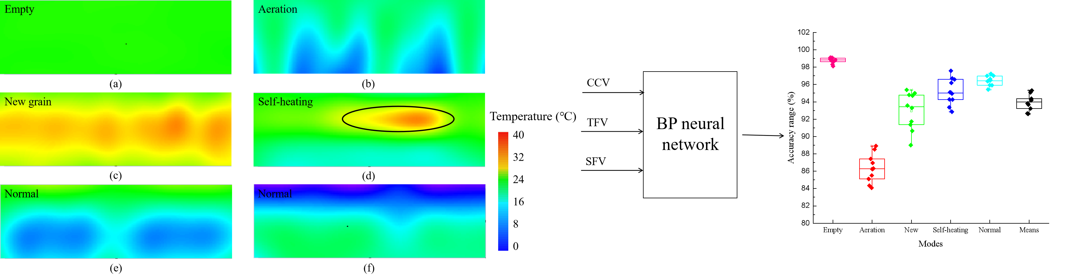
2.1. Virtual Coordinate System of Temperature Sensors and Preprocessing of Temperature Data

In order to generate temperature contour maps, a virtual coordinate system was first established to define the locations of temperature sensors (Figure 1a), with m_x, n_y and l_z representing the temperature measurement points in the X, Y and Z directions, respectively. Temperature sensors were grouped based on the planes that are parallel to XY, XZ, and YZ planes, respectively. For example, 108 sensors in a grain storage warehouse formed 4 planes (layers) parallel to the XY plane, 3 planes to the XZ plane and 9 planes to the YZ plane, as shown in Figure 1.

Outliers (or missing points) in the temperature data that affected the generation of temperature contour maps were mostly caused by software and hardware (sensors) failure. These outliers typically appeared as values exceeding the physically possible temperature range (e.g., 99 °C), or simply a non-numerical error code. Once found, we first determined the location (m_x, n_y, l_z) and time t3 where and when the outliers occurred. After that, we selected the temperature T (m_x, n_y, l_z)_t1 and T (m_x, n_y, l_z)_t2 at the two adjacent times t2 and t1 before t3, and then calculated the temperature T (m_x, n_y, l_z)_t3 by Equation (1).

$$T{(m_x,n_y,l_z)}_{t3}=T{(m_x,n_y,l_z)}_{t2}+\frac{T{(m_x,n_y,l_z)}_{t2}-T{(m_x,n_y,l_z)}_{t1}}{t2-t1}$$

(1)

Typically, direction of airflow during aeration is upward from the bottom of grain bulk, so it is expected that large temperature changes would occur in the planes parallel to YZ or XZ. Since the planes parallel to XZ contained more temperature sensors, it was selected to generate temperature contour maps (Figure 1b). It should be noted that no sensors were installed near the wall in a typical grain warehouse and the grain temperatures near the wall (points 2 in Figure 1b) were extrapolated from the temperatures of three consecutive adjacent points (points 1). Similarly, the average temperature of two adjacent points (points 2) was used to approximate the grain temperature at the corner (point 3).

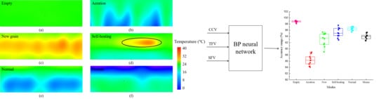
2.2. Generation of RGB Temperature Contour Maps

The discrete temperature data points consisted of the measured temperature values and the approximated values near the walls were interpolated by using splines to generate a temperature contour map. The temperatures from the minimum to the maximum were divided into 765 grades for the (R, G, B) color intervals. The color (R, G, B) values corresponding to the maximum temperature were assigned (255, 0, 0), and the minimum (0, 0, 255) [30]. Then, a RGB temperature contour map for each plane with a resolution of 496 × 158 pixels was generated.

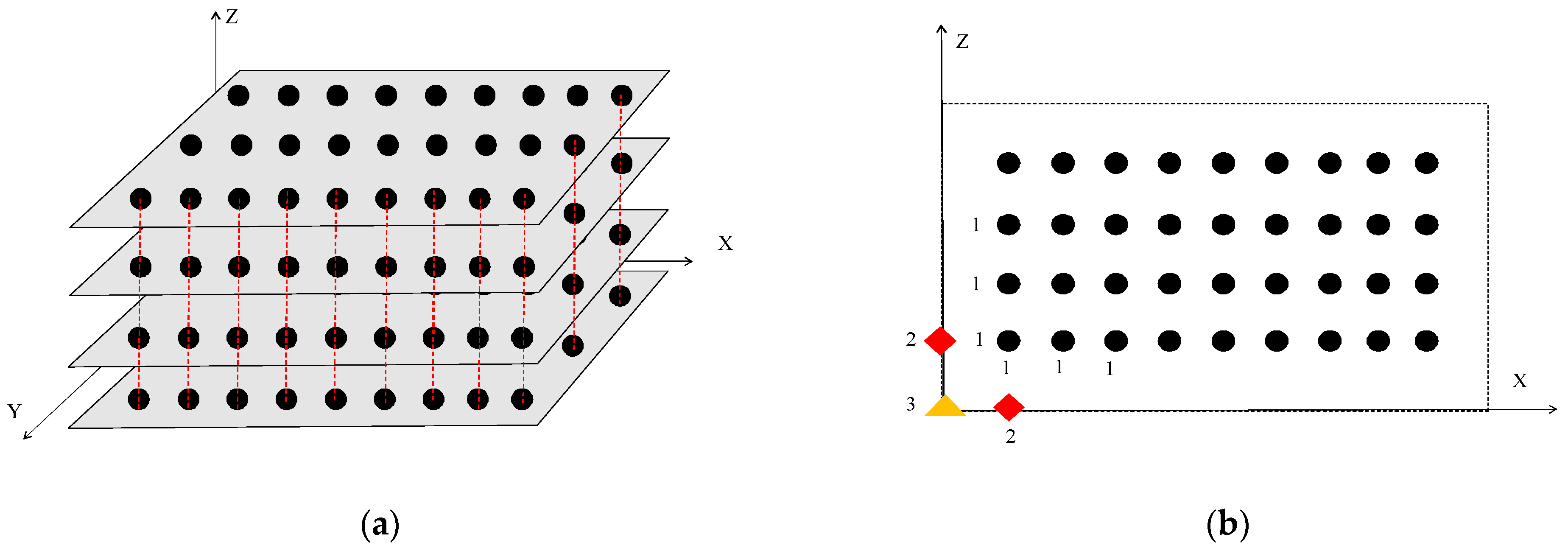
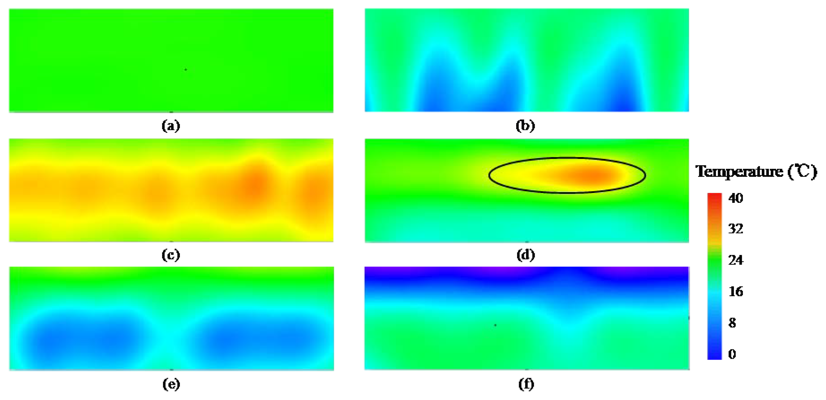
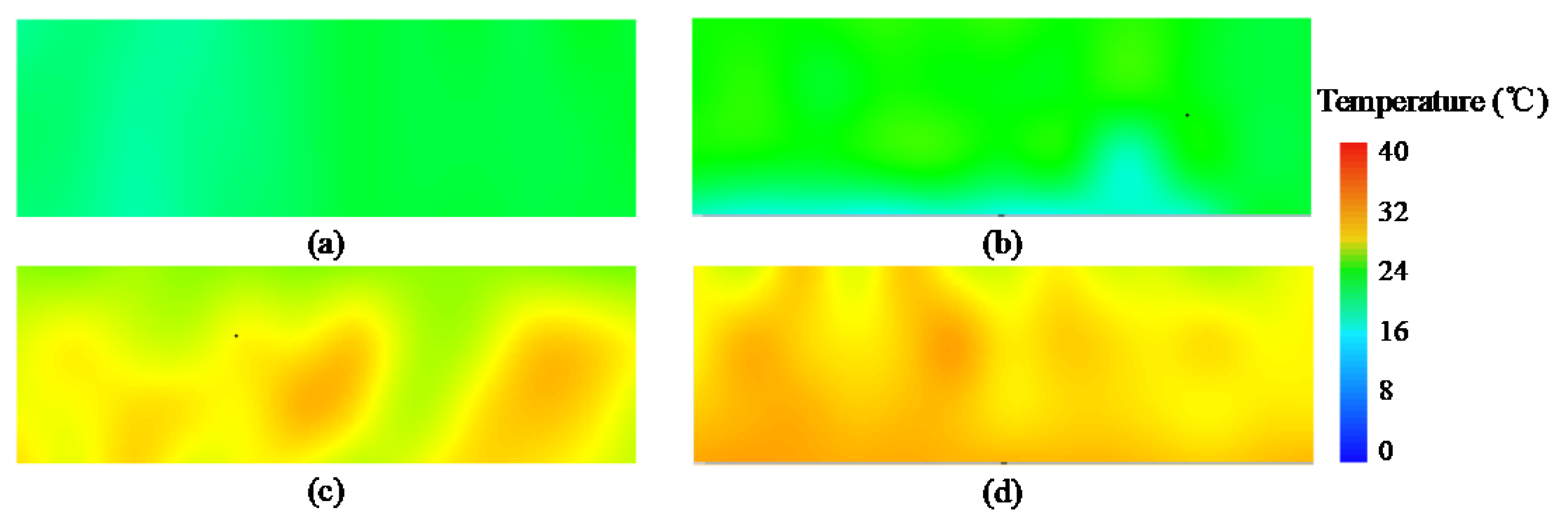
2.3. Classification of Storage Conditions

The storage period of grain is usually more than 6 months in China [31]. Grain conditions changes are shown in Figure 2. When a shipment arrives, grain is loaded into an empty warehouse till it is filled. Then, grain stays in the warehouse for the entire storage period. During storage, grain conditions may change due to the effects of ambient environment and physical (e.g., aeration) and biological (e.g., mold growth) activities within the grain bulk. After about 2–4 years of storage, grain is unloaded from the warehouse (the warehouse returns to being empty again).

According to Figure 2, the storage conditions of grain in a warehouse may be categorized into five modes: normal, empty (warehouse), new grain addition, aeration, and self-heating. These five modes are reflected by the temperature distribution (spatial) and variation (temporal) patterns. Specifically, the empty mode corresponds to uniform temperature distribution through the warehouse (Figure 3a); aeration resulted in the rapid change of temperatures in local areas or the whole grain bulk (Figure 3b). New grain addition indicates that grain was just loaded into an empty warehouse. After a while when the warehouse was filled, the grain temperature at the bottom and surface has dropped. But grain temperature in the middle was still very high. Then a hot core that ran through the entire grain bulk formed in the middle of the contour map (Figure 3c). This condition was named as new grain addition. The self-heating mode is associated with increased temperature in the local region due to biological activities such as mold and insect’s growth (Figure 3d). Several temperature patterns existed for the normal storage conditions which depended on several factors, including the geographical location, the time and the type of warehouse (Figure 3e,f). From spring to summer, the surrounding area of grain bulk was affected by the external temperature, where temperature rises faster and the temperature inside rose slowly. Until summer, the contour map was characterized by high temperature at the surrounding area of the grain bulk, and a cold core formed at the bottom of the contour map (Figure 3e). From summer to winter, the temperature around the grain bulk decreased rapidly. But inside the grain bulk decreased slowly. Until winter, it was characterized by low temperatures at the surrounding areas. Then a hot core formed at the bottom of the grain bulk (Figure 3f). Contour maps in the spring and autumn are also normal mode.

2.4. Datasets for Training and Validation

Grain temperatures data were obtained from 37 flat grain storage warehouses from the second to the seventh stored grain ecological regions between 1 June 2017 and 1 December 2018. Different grain storage warehouses used different types of temperature measurement sensors from different manufacturers. The sensors had accuracies typically within 1 °C, as per the National Standards of the People’s Republic of China [9]. The types of grains stored in these warehouses included corn, wheat and paddy. Those warehouses are located at 23–53° north latitude and 101–133° east longitude, and most of them are located in the subtropical monsoon climate and temperate monsoon climate. Grain temperature data of different inventory modes were selected. After that, the sample set of temperature contour map data was generated by the methods in Section 2.1 and Section 2.2. The sample set was composed of 4000 temperature contour maps of empty mode, 2800 temperature contour maps of aeration mode, 1400 temperature contour maps of new grain addition, 1500 temperature contour maps of self-heating mode and 8000 temperature contour maps of normal mode. In order to train the network, the labels of the empty mode, new grain addition, aeration, self-heating and normal mode were set as 1, 2, 3, 4 and 5, respectively. In different literatures, researchers set different proportions of training samples and test samples, such as 70:30 [32], 80:20 [33]. Taking into account the diversity of temperature contour maps, in this study we increased the proportion of training samples to 85% of the total dataset, and the remaining proportion (15%) was the test samples.

2.5. Features Extraction of Temperature Contour Maps

A key step in using a BP neural network to classify the grain conditions during storage is selecting the suitable input to the network. Several features of the RGB temperature contour maps are considered, including the color, texture and smoothness features.

2.5.1. Color Coherence Vector Extraction

As can be seen from Figure 3, there are noticeable differences in the color features of different modes. Thus, color feature was considered to classify the modes. In the color feature, the color distribution histogram is often extracted to reflect the color feature distribution of the image, but the color distribution histogram ignores the position information of the color in the image, so the color coherence vector (CCV) was selected to analyze the color feature of the temperature contour map. Pass proposed a color coherence vector for analyzing the spatial distribution of color [34,35]. The first step is to quantize the image into N bins with the uniform quantization method. Then, the quantized image is divided into several connected regions. If pixels in connected regions are greater than the given threshold, they are treated as coherent pixels; otherwise, incoherent pixels. Based on the above procedures, the color coherence vector of a RGB temperature contour map could be expressed as $\langle ({\alpha }_1,{\beta }_1),({\alpha }_2,{\beta }_2),\dots ({\alpha }_N,{\beta }_N)\rangle$, where α_x and β_x represent the number of coherent pixels and incoherent pixels in the x_th bin, respectively. In order to easily combine with other feature vectors, the color coherence vector was expressed as $\langle {\alpha }_1,{\beta }_1,{\alpha }_2,{\beta }_2,\dots {\alpha }_N,{\beta }_N\rangle$. To minimize the color loss in the quantization process, we set the range of N between [60, 80] according to the discussion of literature [36]. The CCV was extracted from each sample, and concatenated into a matrix with 2 N columns, which was used as the input of the network alone or combined with other matrices as the input matrix of the network.

2.5.2. Texture Feature Extraction

A statistical method is used to calculate the area with multiple pixels to analyze the statistical law of the image, which is suitable for irregular arrangement. The arrangement of texture features of the temperature contour map was not regular, so in this study, we selected and extracted several commonly used statistical features in a gray histogram as the texture feature vector. Texture features of the image histogram commonly used include the gray mean M, variance ${\sigma }^2$, standard deviation s, skewness S, kurtosis K, and entropy ER, whose definitions and calculation methods can be found in the literature [37,38,39]. These six features of each component’s histograms (three component histogram R, G, B in each RGB temperature contour map) were extracted and connected, respectively. Then, they formed a texture feature vector (TFV) with 18 elements. The TFV was extracted from all contour maps and concatenated into a matrix with 18 columns that were used as the input matrix of the network alone or combined with other matrices as the input matrix of the network.

2.5.3. Smoothness Feature Extraction

It can be seen from Figure 3 that the temperature contour map of the empty mode is smoother than that of other modes. Therefore, the characteristics that can represent the smoothness of the image were selected to analyze the temperature contour map. Smoothness usually represents the smoothness level/roughness of image intensity. Different studies have different definitions of smoothness. Sinaga defined features S_m as the smoothness of color histograms [40] and Deutsch used O_s to define it [41]. In this research, these two features of each component’s histogram were extracted respectively and formed the smoothness feature vector (SFV) with 6 elements. The SFV was extracted from all contour maps and was concatenated into a matrix with 6 columns that was utilized as the input alone, or combined with others as the input matrix of the network.

2.6. Construction of BP Neural Network

As a supervising learning neural networks, the BP neural network is used most widely and successfully to classify image dataset which includes different objects [42,43,44,45]. A BP neural network usually consists of input layer, hidden layer and output layer [46]. Determination of the number of neurons in the hidden layers and each hidden layer is important to define the overall neural network architecture. A considerable amount of literature suggested that a neural network with two hidden layers can approximate any smooth mapping to any accuracy [47]. Therefore, this study designed a four-layer BP neural network in MATLAB toolbox (2016b, MathWorks, Massachusetts, USA), including one input layer, two hidden layers and one output layer. The number of neurons in the input layer was linked to the input matrix, and the best input matrix was determined through experiments. The number of neurons in the output layer was set to five corresponding to the five modes. Based on the numbers of neurons in the input and output layers, the number of neurons in the hidden layers could be calculated by the empirical formula Equation (2) [46].

$$l=\sqrt{m+n}+a$$

(2)

where l is the number of neurons in the hidden layer, n is the number of neurons in the input layer, m is the number of neurons in the output layer, and a is a trial parameter ranging from 1 to 10 [48].

Apart from the number of nodes in the hidden layer, some other training parameters, such as the training function, transfer function, learning rate and momentum coefficient, are related to the training speed and network generalization capability as well [46]. The ‘Levenbverg_Marquardt’ trainlm was selected as the training function, and ‘Log-Sigmoid function’ was used as transfer function [49], and the learning rate, momentum coefficient and target error were set to 0.01, 0.9 and 0.0001, respectively through preliminary comparing experiments [48,50]. The hardware environment of the models and programs running in this study is Thinkpad X1 Extreme (Lenovo, Beijing, China), whose system version is Win 10-64, and processor is Intel Core (TM) i5-9300H CPU 2.40 GHz.

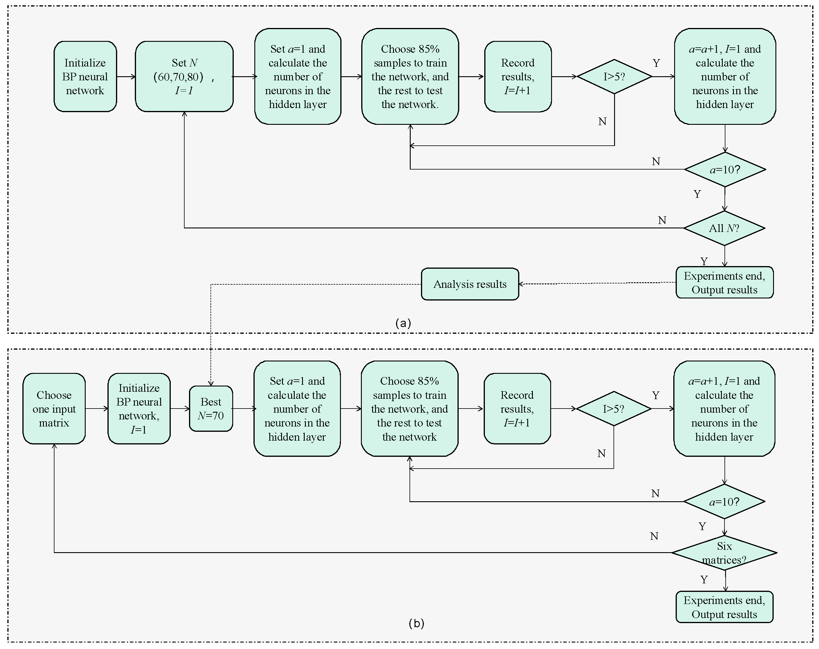
2.7. Experiments Method

2.7.1. Optimization Experiments of Neural Network Input

Many researchers have analyzed the influence of input matrix on prediction accuracy [51]. To optimize input matrix for better classification accuracy, training time (time for the network to complete training) and prediction time (time for the network to predict), six matrices were used as the input matrix of BP neural network individually and sequentially, including CCV, TFV, SFV, combination matrix of CCV and TFV (CCV&TFV), combination matrix of CCV and SFV (CCV&SFV) and combination matrix of CCV and TFV and SFV (CCV&TFV&SFV).

Since the number of N (CCV quantified the image into N bins) had an effect on the accuracy of the network, we first adjusted N to 60, 70, 80 successively to calculate CCV, and then combined it with TFV and SFV as input matrix to conduct experiments. The procedure is shown in Figure 4a and results are presented in Figure 5. After the most suitable N was selected, we used the above six matrices to perform optimization experiments for better input matrix. The procedure is shown in Figure 4b and the results are shown in Figure 6 and Figure 7. During all experiments, the training time and prediction time were recorded.

2.7.2. Classification Experiments of Neural Network

According to optimization experimental results, combination matrix of CCV (N = 70), TFV and SFV was chosen as the input matrix of the neural network. Classification experiments by BP neural network were conducted 10× since a was from 1 to 10. After a test ended, we reset a value to obtain a new and different number of neurons in the hidden layer. Then, the test was repeated five times again, and the average of results was considered as the results of the classification experiment with the a value.

2.7.3. Comparative Experiment

The support vector machine (SVM) is also a commonly used classification method [52,53]. Thus, SVM was chosen as the method of comparative experiments. A library for support vector machine (LIBSVM) is an integrated software for support vector classification, regression and distribution estimation [54]. The function ‘svmtrain’ in it was used to classify the five grain inventory modes. The kernel function of SVM chose the function ‘linear’, ‘polynomial’ and ‘radial basis’. Five tests were conducted for each kernel function.

3. Results and Discussion

3.1. Optimization Experiments Results of Neural Network Input

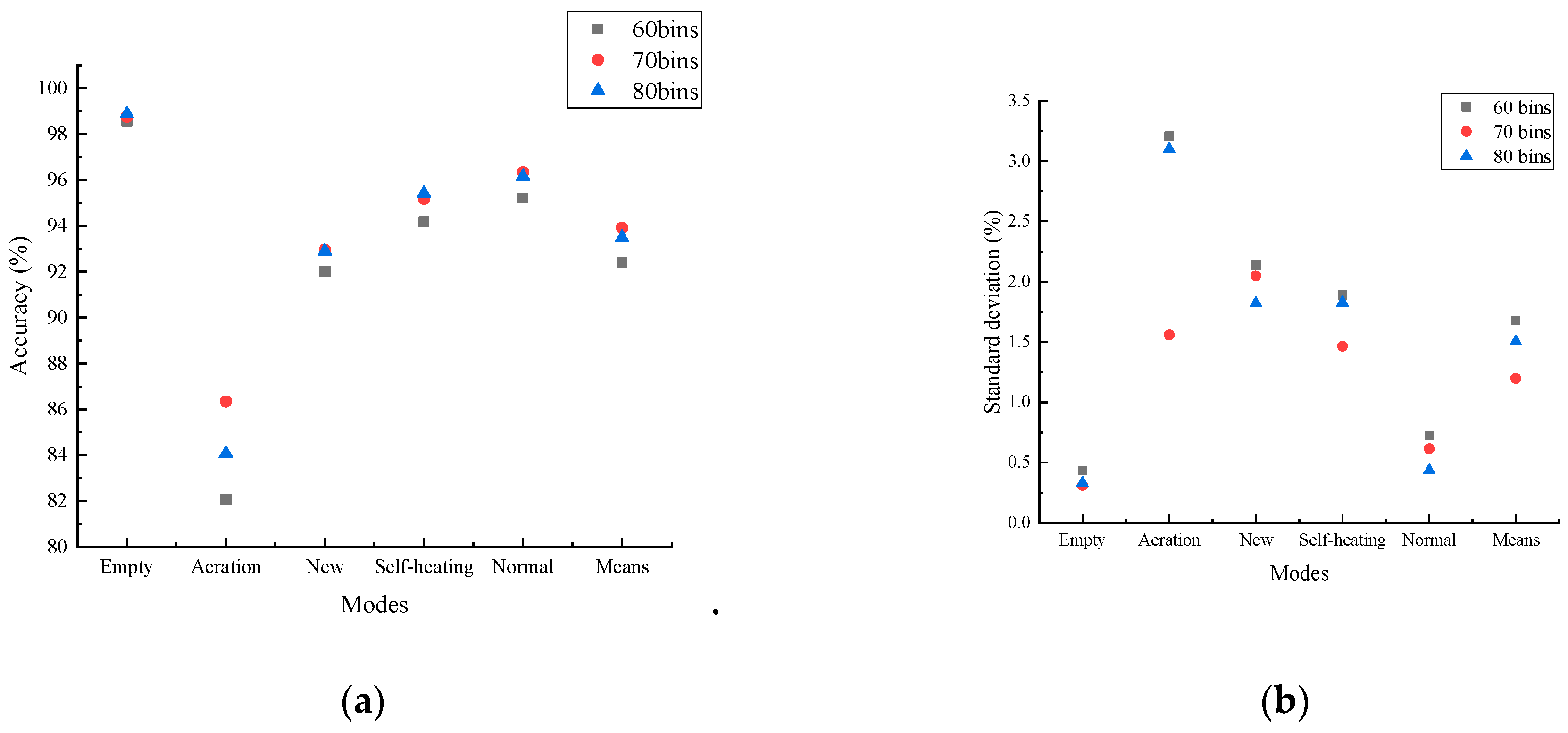
3.1.1. Effect of Color Quantification on Classification Accuracy

To assess the effect of the number N of color quantification bins in CCV on classification accuracy, colors were quantified into 60, 70 and 80 bins. Combination of CCV, TFV and SFV was used as the input matrix. The results are shown in Figure 5.

Figure 5a shows that classification accuracies of empty mode are the highest (about 98%) when colors are quantized into 60, 70, and 80 bins, that of aeration mode is the lowest (about 84%) and that of new grain addition, self-heating and normal is between 91–96%. Figure 5b shows that standard deviation of classification accuracies of empty mode is the lowest (only about 0.4%). However, for aeration mode, the standard deviation of classification accuracies is obviously different when colors are quantized into 60, 70, and 80 bins, and among them, standard deviation when 70 bins is the lowest (about 1.5%) and standard deviations when 60 and 80 bins are the same (about 3.2%). Figure 5 also shows that when colors are quantized into 60 bins, classification accuracies are the lowest except for the empty mode and the standard deviations of classification accuracies are higher than that when 70 and 80 bins. This is due to the fact that the smaller number of bins could not contain widely distributed colors. However, too many bins may contain too much noise, resulting in lower classification accuracies and higher standard deviation of classification accuracies, which is evidenced by the difference between 70 and 80 bins for aeration mode in Figure 5. It also can be seen that, when colors are quantized into 70 bins, the mean of classification accuracy is the highest and standard deviation is lowest. Thus, when colors were quantified into 70 bins, CCV&TFV&SFV could make the neural network get better classification results. It appeared that 70-bin color quantification was optimal in this study.

3.1.2. Effect of Training Features on Classification Accuracy

To optimize the input matrix for better classification accuracy, training time and prediction time, the six combinations of the input matrix (CCV (70 bins), TFV, and SFV) were tested. The results are shown in Figure 6.

Figure 6 shows that accuracies are the highest (near 99%) when CCV&TFV&SFV or CCV&TFV is the input matrix, and no noticeable differences between these two combinations. This is owing to the fact that the distinguishes between these two matrices CCV&TFV&SFV (CCV 140 columns + TFV 18 columns + SFV 6 columns) and CCV&TFV (CCV 140 columns + TFV 18 columns) is SFV (6 columns) that contains much less image information that it has little influence on accuracy. This also can explain why the classification accuracies are the lowest when only SFV is used as the input matrix (except for new grain addition), and why the classification accuracies when CCV&SFV is the input matrix are slightly higher than that when CCV is alone. In particular, for new grain addition, classification accuracy when SFV is the input matrix is slightly higher than that when TFV is. This is owing to the fact that SFV contains more representative features for new grain addition since most of temperature contour maps of new grain addition is not smooth because of grain loaded in different ways at different times, while for other modes, the features SFV contained are not representative.

The computation time is an important factor to be considered when a large amount of grain temperature data need to be processed to offer timely on-site assessment of grain conditions. Additionally, if new (different) datasets suddenly became available on-site, the BP neural network would need to be retrained in a limited time. Thus, training times and prediction times of neural network with different input matrices were measured when experiments were done.

From Figure 7, it can be seen that when CCV&TFV&SFV is the input matrix, training time and prediction time are the highest, which are about 320 and 0.12 s respectively. In addition, when CCV&TFV is the input matrix, training time and prediction time are slightly smaller than that when CCV&TFV&SFV. Additionally, when SFV is the input matrix, training time and prediction time are the smallest, which are 10 and 0.11 s. Figure 7 also shows that prediction time for different input matrices is between 0.11 and 0.12 s (the difference can be ignored). It should be noted that when the number of neurons in the input layer decreases, both training time and prediction time decreases. The decrease of the number of columns in the input matrix was equivalent to the decrease of the number of neurons in the input layer. Thus, input matrices affected the training time and prediction time. It can interpret why training and prediction time increase with the increase of the number of neurons in the input layer.

Combined classification accuracies and times are shown in Figure 6 and Figure 7, whereby it should be noted that increasing the number of neurons in the input layer would prolong the training time, while its classification accuracy would be higher. Simultaneously, it can be noted that the accuracies are very similar when CCV&TFV&SFV and CCV&TFV are the input matrix, while training time of CCV&TFV is shorter (the difference can be ignored). Thus, if the network was to be retrained on site, CCV&TFV could be chosen as the input matrix for economizing in time. In summary, the BP neural network with CCV&TFV&SFV or CCV&TFV as inputs possessed better accuracy, and the training time and prediction time were about 320 and 0.12 s, respectively.

3.2. Classification Accuracy

According to the training results of neural network in the above section, CCV&TFV&SFV was chosen as the input matrix of the BP neural network. The classification results are shown in Figure 8. When constant a was re-selected from 1 to 10, the number of hidden layer neurons was reset. Thus, ten experiments were done. Classification accuracies of ten experiments are shown in Figure 8 and

Table 1. Analysis of classification accuracies when constant a was selected from 1 to 10.

Constant a	1	2	3	4	5	6	7	8	9	10
Accuracy (%)	92.61	92.66	93.22	94.26	94.36	93.67	95.32	95.07	94.17	93.81
SD (%)	4.32	4.56	4.23	3.76	3.94	4.51	3.42	4.28	5.09	5.14

Note: “SD” represents the standard deviation, %.

.

From all the boxes in Figure 8, the classification accuracy for empty mode is the highest (>98%). It is due to the fact that color distribution of the contour maps of empty mode is relatively monotonous, which is obviously different from the contour maps of other modes. In addition, the aeration is the lowest (82–89%), which is due to the fact that color distribution of the contour maps of aeration mode is influenced by many factors, such as the aeration time, the location of grain warehouse, the external air temperature during aeration and so on. Thus, temperature contour maps of aeration mode are so different that the accuracies are the lowest. The accuracies for new grain addition, self-heating and normal mode range between 89% and 98%, and the mean accuracies are about 93.9% in Figure 8. From the upper and lower limits of all boxes in Figure 8, it can be seen that the height of box is the smallest for empty mode and the highest for new grain addition, which means that the fluctuation of accuracies was the smallest for empty mode and highest for new grain addition. The reason that caused the accuracies fluctuated greatly is that the training samples were reselected as the number of hidden layer neurons reset (since constant a was reset from 1 to 10). The color distribution of the contour maps of empty mode was so different from that of other modes that the training samples of empty mode, selected before and after, had less effect on the classification accuracy (smallest fluctuation). The contour maps of new grain addition were quite different from each other, which is due to the time and method for grain loaded into the warehouse, thus the training samples selected before and after were very different, which lead to a large fluctuation of classification accuracies.

Table 1 demonstrates that different a make classification accuracies and standard deviations of five modes of the BP neural network different. Among the results, when constant a was 1, the average of classification accuracies of five modes was the lowest at about 92.61%. In addition, when constant a was 7, the average of classification accuracies was the highest at about 95.32%, and the standard deviation was smallest (about 3.42%). Thus, constant a was set as 7. Then the most suitable number of hidden layer neurons was 20. When constant a was 7, the BP neural network owned the best classification effect with accuracies of 99.10%, 88.91%, 95.37%, 96.59% and 96.62% for the five modes. Examples of the inaccurate classification are shown in Figure 9.

All the temperature sensors measured similar air temperatures when the warehouse was empty. That formed temperature contour maps with a uniform color (Figure 9a). This uniform pattern could be easily identified, resulting in a high accuracy. Some temperature contour maps for aeration (Figure 9b) were similar to the empty mode, which lead to misclassification of the aeration to the empty mode, and vice versa. A temperature contour map of new grain addition may be misclassified as self-heating (Figure 9c) since temperatures of new grain could be higher than 35 °C at the time when grain was just loaded into the warehouse in the summer. The temperature contour map (Figure 9d) of self-heating mode was misidentified as that of new grain addition. The reason is that grain temperature was still very high (beyond 35 °C) one month after grain loaded, and temperature contour maps at the time were similar with that of new grain addition.

3.3. Comparative Experimental Results

The classification results with the SVM are shown in

Table 2. Classification results with the SVM.

Kernel Function	Empty (%)		Aeration (%)		New (%)		Self-Heating (%)		Normal (%)		Overall (%)
	Mean	SD	Mean	SD	Mean	SD	Mean	SD	Mean	SD	Mean	SD
Linear	88.6	1.2	76.0	2.0	68.4	2.8	80.9	3.0	78.6	0.6	80.2	0.8
Radial basis	94.0	1.1	91.3	0.8	87.2	1.5	92.3	1.6	91.1	0.6	91.6	0.6
Polynomial	93.1	1.4	92.3	1.8	87.7	2.7	92.5	1.9	93.4	0.4	92.6	0.6

Note: Linear, polynomial and radial basis represent the kernel function of support vector machine [55]. “SD” represents the standard deviation.

to compare with the results of the BP network.

Classification accuracies of the SVM with the linear kernel function were lower than 90% for all five modes, and the polynomial and radial kernel functions resulted in classification accuracies around 91.6% and 92.6%, respectively. Through comparison with Figure 8, accuracies of the BP neural network (overall accuracy about 93.9%) were higher than that of the SVM, except for the aeration mode when the polynomial and radial kernel functions were used. The training time and prediction time of SVM were 25.6 and 5.02 s, respectively. Then, the training time of the BP neural network (320 s) was longer than that of SVM, and prediction time (0.12 s) shorter than that of SVM.

Considering the accuracy, training time and prediction time, the BP neural network needs to obtain a large number of image samples in advance and complete the training of the network before application. After arriving at the detection site, the trained network can be directly used, which can save training time and possess a higher accuracy. In addition, grain temperatures data in this study were obtained from 37 flat grain storage warehouses. Since China’s grain depots are widely distributed, temperature contour maps in the different regions are different. In the future, more grain temperature data could be obtained to generate more temperature contour maps in order to test or improve the accuracy of the BP neural network.

4. Conclusions

A back propagation (BP) neural network was presented to classify the grain conditions, including inventory changes and routine operations performed (aeration), based on the temperature contour map of the stored grain. The grain inventory modes were categorized into five modes, namely, empty (no grain in storage), aeration, new grain addition, self-heating and normal conditions, with which the temperature contour maps sample set was established. The color coherence vector (CCV), texture feature vector (TFV) and smoothness feature vector (SFV) of the temperature contour map were extracted and combined as the input of the BP neural network, and the five modes were used as the output vector. The experimental results showed that classification accuracy for the empty mode was the highest (>98%) and the aeration the lowest (82–89%). The accuracies for the new grain addition, self-heating and the normal mode ranged between 89% and 98%, with a mean accuracy about 93.9%. The results also showed that the BP neural network with CCV&TFV&SFV or CCV&TFV as input possessed better accuracy, and its training time and prediction time were about 320 and 0.12 s, respectively. Comparative experimental results showed that the BP neural network had slightly better classification accuracies than the SVM (93.9% vs. 92.6% on average) and a shorter prediction time (0.12 vs. 5.02 s), but a longer training time (320 vs. 25.6 s). In the future, more grain temperatures from more different grain depots could be collected to generate more temperature contour maps in order to improve the accuracy of the BP neural network.

References

1. Zhang, C.; Tian, X.G.; He, R.; Ju, X.R.; Yuan, J.; Song, X.Y. Causes and research progress of condensation in grain heap. Grain Storage 2018, 47, 1–5. [Google Scholar]
2. Xue, F.; Qu, C.; Wang, R.W.; Li, H.L. Progress on the fever and moldy of paddy during storage. Sci. Technol. Food Ind. 2016, 38, 338–340. [Google Scholar]
3. Yang, S.; Cao, Y.; Zhao, H.; Fei, M. Research progress of rapid detection technology in grain mildew. Grain Oil 2018, 31, 21–23. [Google Scholar]
4. Zhang, Y.Y.; Cai, J.P.; Jiang, P. Detection techniques for mold harm activities in stored-grain. Food Mach. 2013, 29, 267–272. [Google Scholar]
5. Geng, Z.F.; Liu, Z.L.; Wang, C.F.; Liu, Q.Z.; Shen, S.M.; Liu, Z.M.; Du, S.S.; Deng, Z.W. Feeding Deterrents against Two Grain Storage Insects from Euphorbia fischeriana. Molecules 2011, 16, 466–476. [Google Scholar] [CrossRef] [Green Version]
6. Liu, S.S.; Arthur, F.H.; VanGundy, D.; Phillips, T.W. Combination of Methoprene and Controlled Aeration to Manage Insects in Stored Wheat. Insects 2016, 7, 25. [Google Scholar] [CrossRef] [Green Version]
7. Wang, S.; Wu, T.; Shao, T.; Peng, Z. Integrated model of BP neural network and CNN algorithm for automatic wear debris classification. Wear 2019, 426, 1761–1770. [Google Scholar] [CrossRef]
8. Manandhar, A.; Milindi, P.; Shah, A. An Overview of the Post-Harvest Grain Storage Practices of Smallholder Farmers in Developing Countries. Agriculture 2018, 8, 57. [Google Scholar] [CrossRef] [Green Version]
9. China National Standards Management Committee. Technical criterion for grain and oil-seeds storage-GB/T 29890-2013; China Standards Press: Beijing, China, 2013. [Google Scholar]
10. Nie, Z.B. Director of the State Administration of Grain, Answers Questions about the “Interim Measures for the Inspection of Grain Stocks” on the Chinese Government Website. 2006. Available online: http://www.gov.cn/ztzl/yzn/content_479484.htm (accessed on 26 October 2020).
11. Xiao, Q. Research on the Strategies and Methods of Storing Grain Digital Supervision Based on the Grain Monitoring; Jilin University: Changchun, China, 2018. [Google Scholar]
12. Cui, H.; Wu, W.; Wu, Z.; Han, F.; Zhu, H.; Qin, X. Reserves monitoring method for grain storage based on temporal and spatial correlation of grain temperature. Trans. Chin. Soc. Agric. Mach. 2019, 50, 321–330. [Google Scholar]
13. Cui, H.W.; Wu, W.F.; Wu, Z.D.; Han, F. A Method for Detecting Abnormal Changes in the Temperature Field of Grain Bulk Based on HSV Features of Cloud Maps. Trans. ASABE 2020, 63, 1181–1191. [Google Scholar]
14. Zheng, Y.; Li, G.; Li, Y. Survey of application of deep learning in image Recognition. Comput. Eng. Appl. 2019, 55, 20–36. [Google Scholar]
15. Chen, Y.; Huang, L.; Zhu, L.; Yokoya, N.; Jia, X. Fine-grained classification of hyperspectral imagery based on deep learning. Remote Sens. 2019, 11, 2690. [Google Scholar] [CrossRef]
16. Yin, C.; Chen, Z. Developing sustainable classification of diseases via deep learning and semi-supervised learning. Healthcare 2020, 8, 291. [Google Scholar] [CrossRef] [PubMed]
17. Ragab, D.A.; Sharkas, M.; Marshall, S.; Ren, J. Breast cancer detection using deep convolutional neural networks and support vector machines. PeerJ 2019, 7, e6201. [Google Scholar] [CrossRef] [PubMed]
18. Costa, N.L.; Llobodanin, L.A.G.; Castro, I.A.; Barbosa, R. Geographical classification of tannat wines based on support vector machines and feature selection. Beverages 2018, 4, 97. [Google Scholar] [CrossRef] [Green Version]
19. Fan, Y.; Wang, B.; Wang, W.; Tang, Y. A Summary of Research on Deep Learning in China. Distance Educ. China 2015, 6, 27–33+79. [Google Scholar]
20. Li, J.; Pan, Z. Network Traffic Classification Based on Deep Learning. KSII Trans. Internet Inf. Syst. 2020, 14, 4246–4267. [Google Scholar]
21. Chen, Y.; Wang, Y.; Gu, Y.; He, X.; Ghamisi, P.; Jia, X. Deep Learning Ensemble for Hyperspectral Image Classification. IEEE J. Sel. Top. Appl. Earth Obs. Remote Sens. 2019, 12, 1882–1897. [Google Scholar] [CrossRef]
22. Liu, P.; Zhang, H.; Eom, K.B. Active Deep Learning for Classification of Hyperspectral Images. IEEE J. Sel. Top. Appl. Earth Obs. Remote Sens. 2017, 10, 712–724. [Google Scholar] [CrossRef] [Green Version]
23. Cervantes, J.; Garcia-Lamont, F.; Rodríguez-Mazahua, L.; Lopez, A. A comprehensive survey on support vector machine classification: Applications, challenges and trends. Neurocomputing 2020, 408, 189–215. [Google Scholar] [CrossRef]
24. Zhang, Y. Support Vector Machine Classification Algorithm and Its Application. In Information Computing and Applications; Pt II; Liu, C.F., Wang, L.Z., Yang, A.M., Eds.; Springer: Berlin/Heidelberg, Germany, 2012; pp. 179–186. [Google Scholar]
25. Wang, Y.; Wang, J.; Chang, S.; Sun, L.; An, L.; Chen, Y.; Xu, J. Classification of Street Tree Species Using UAV Tilt Photogrammetry. Remote Sens. 2021, 13, 216. [Google Scholar] [CrossRef]
26. Zhou, F.; Su, Z.; Chai, X.; Chen, L. Detection of Foreign Matter in Transfusion Solution Based on Gaussian Background Modeling and an Optimized BP Neural Network. Sensors 2014, 14, 19945–19962. [Google Scholar] [CrossRef] [PubMed] [Green Version]
27. Wu, S.; Liu, J.; Yu, Y. Prediction of cut size for pneumatic classification based on a back propagation (BP) neural network. ZKG Int. 2016, 69, 64–71. [Google Scholar]
28. Huang, Y.; Meng, S.; Hwang, S.; Kobayashi, K.; Sugiyama, J. Neural Network for Classification of Chinese Zither Panel Wood via Near-infrared Spectroscopy. BioResources 2020, 15, 130–141. [Google Scholar]
29. Yuan, C.; Sun, X.; Wu, Q.J. Difference co-occurrence matrix using BP neural network for fingerprint liveness detection. Soft Comput. 2019, 23, 5157–5169. [Google Scholar] [CrossRef]
30. Cui, H.W.; Wu, W.F.; Wu, Z.D.; Han, F. Monitoring method of stored grain quantity based on temperature field cloud maps. Trans. Chin. Soc. Agric. Eng. 2019, 35, 290–298. [Google Scholar]
31. Duan, S.; Yang, W.; Wang, X.; Mao, S.; Zhang, Y. Grain pile temperature forecasting from weather factors: A support vector regression approach. In Proceedings of the 2019 IEEE/CIC International Conference on Communications in China (ICCC), Changchun, China, 11–13 August 2019. [Google Scholar]
32. Gholami, V.; Chau, K.; Fadaee, F.; Torkaman, J.; Ghaffari, A. Modeling of groundwater level fluctuations using dendrochronology in alluvial aquifers. J. Hydrol. 2015, 529, 1060–1069. [Google Scholar] [CrossRef]
33. Alqahtani, A.; Whyte, A. Artificial neural networks incorporating cost significant items towards enhancing estimation for (life-cycle) costing of construction projects. Constr. Econ. Build. 2013, 13, 51–64. [Google Scholar] [CrossRef] [Green Version]
34. Pass, G.; Zabih, R.; Miller, J. Comparing images using color coherence vectors. In Proceedings of the Fourth ACM International Multimedia Conference, Boston, MA, USA, 1 February 1997. [Google Scholar]
35. Moslehi, M.; de Barros, F.P. Using color coherence vectors to evaluate the performance of hydrologic data assimilation. Water Resour. Res. 2019, 55, 1717–1729. [Google Scholar] [CrossRef]
36. Ramella, G.; Di Baja, G.S. A new method for color quantization. In Proceedings of the 2016 12th International Conference on Signal-Image Technology & Internet-Based Systems (SITIS), Naples, Italy, 28 November–1 December 2016. [Google Scholar]
37. Djemal, R.; AlSharabi, K.; Ibrahim, S.; Alsuwailem, A. EEG-based computer aided diagnosis of autism spectrum disorder using wavelet, entropy, and ANN. BioMed Res. Int. 2017, 2017, 9816591. [Google Scholar] [CrossRef] [Green Version]
38. Vécsei, A.; Fuhrmann, T.; Uhl, A. Towards automated diagnosis of celiac disease by computer-assisted classification of duodenal imagery. In Proceedings of the 4th IET International Conference on Advances in Medical, Signal and Information Processing (MEDSIP 2008), Santa Margherita Ligure, Italy, 14–16 July 2008. [Google Scholar]
39. Navarro, C.F.; Perez, C.A. Color—Texture pattern classification using global—Local feature extraction, an SVM classifier, with bagging ensemble post-processing. Appl. Sci. 2019, 9, 3130. [Google Scholar] [CrossRef] [Green Version]
40. Sinaga, A.S. Texture Features Extraction of Human Leather Ports Based on Histogram. Indones. J. Artif. Intell. Data Min. 2018, 1, 92–98. [Google Scholar] [CrossRef] [Green Version]
41. Deutsch, C.V. Constrained smoothing of histograms and scatterplots with simulated annealing. Technometrics 1996, 38, 266–274. [Google Scholar] [CrossRef]
42. Liu, P.; Zhang, W. A fault diagnosis intelligent algorithm based on improved bp neural network. Int. J. Pattern Recognit. Artif. Intell. 2019, 33, 1959028. [Google Scholar] [CrossRef]
43. Cao, J.; Chen, L.; Wang, M.; Shi, H.; Tian, Y. A Parallel Adaboost-Backpropagation Neural Network for Massive Image Dataset Classification. Sci. Rep. 2016, 6, 38201. [Google Scholar] [CrossRef] [Green Version]
44. Zhang, C.W.; Chen, S.R.; Gao, H.B.; Xu, K.J.; Yang, M.Y. State of Charge Estimation of Power Battery Using Improved Back Propagation Neural Network. Batteries 2018, 4, 69. [Google Scholar] [CrossRef] [Green Version]
45. Liang, P.; Shi, W.; Zhang, X. Remote Sensing Image Classification Based on Stacked Denoising Autoencoder. Remote Sens. 2017, 10, 16. [Google Scholar] [CrossRef] [Green Version]
46. Wang, L.; Wang, P.; Liang, S.; Qi, X.; Li, L.; Xu, L. Monitoring maize growth conditions by training a BP neural network with remotely sensed vegetation temperature condition index and leaf area index. Comput. Electron. Agric. 2019, 160, 82–90. [Google Scholar] [CrossRef]
47. Heaton, J. The Number of Hidden Layers. 2017. Available online: https://www.heatonresearch.com/2017/06/01/hidden-layers.html (accessed on 26 October 2020).
48. Zhao, Z.; Xin, H.; Ren, Y.; Guo, X. Application and comparison of BP neural network algorithm in MATLAB. In Proceedings of the 2010 International Conference on Measuring Technology and Mechatronics Automation, Changsha, China, 13–14 March 2010. [Google Scholar]
49. Qu, S.L.; Sun, Z.F.; Fan, H.F.; Li, K. BP neural network for the prediction of urban building energy consumption based on Matlab and its application. In Proceedings of the 2010 Second International Conference on Computer Modeling and Simulation, Sanya, China, 22–24 January 2010. [Google Scholar]
50. Pan, R.; Gao, W.; Liu, J.; Wang, H. Automatic recognition of woven fabric pattern based on image processing and BP neural network. J. Text. Inst. 2011, 102, 19–30. [Google Scholar] [CrossRef]
51. Wei, Y.; Xia, L.; Pan, S.; Wu, J.; Zhang, X.; Han, M.; Zhang, W.; Xie, J.; Li, Q. Prediction of occupancy level and energy consumption in office building using blind system identification and neural networks. Appl. Energy 2019, 240, 276–294. [Google Scholar] [CrossRef]
52. Huang, Y.; Zhao, L. Review on landslide susceptibility mapping using support vector machines. Catena 2018, 165, 520–529. [Google Scholar] [CrossRef]
53. Zhu, X.; Li, N.; Pan, Y. Optimization Performance Comparison of Three Different Group Intelligence Algorithms on a SVM for Hyperspectral Imagery Classification. Remote Sens. 2019, 11, 734. [Google Scholar] [CrossRef] [Green Version]
54. Chang, C.; Lin, C. LIBSVM: A library for support vector machines. ACM Trans. Intell. Syst. Technol. Cereals Oils Foods 2011, 2, 1–27. [Google Scholar] [CrossRef]
55. Mehdipour, V.; Memarianfard, M. Ground-level O3 sensitivity analysis using support vector machine with radial basis function. Int. J. Environ. Sci. Technol. 2018, 16, 2745–2754. [Google Scholar] [CrossRef]
Figure 1. Temperature measurement sensors distribution in a grain warehouse: (a) Schematic diagram of temperature measurement sensors distribution in the grain warehouse. (b) Calculation process of temperatures near the wall and corner.
Agriculture 11 00451 g001
Figure 2. Grain storage conditions change process.
Agriculture 11 00451 g002
Figure 3. RGB temperature contour maps of different modes. (a) Empty mode, (b) aeration mode, (c) new grain addition, (d) self-heating, (e, f) normal mode.
Agriculture 11 00451 g003
Figure 4. Optimization experiments flow chart of neural network input. (a) Optimization experiments flow chart of the number of N; (b) Optimization experiments flow chart of input matrix.
Agriculture 11 00451 g004
Figure 5. Classification results when colors were quantized into 60, 70, and 80 bins. (a) Classification accuracy when colors were quantized into 60, 70, and 80 bins; (b) standard deviations of classification accuracies. “Empty” represents empty mode. “Aeration” represents aeration mode. “New” represents new grain addition. “Self-heating” represents self-heating mode. “Normal” represents normal mode. “Means” represents means of accuracies. These are the same as below.
Agriculture 11 00451 g005
Figure 6. Classification accuracies of the neural network for different input matrices.
Agriculture 11 00451 g006
Figure 7. Training times and prediction times of the neural network with different input matrices. Different input matrices can represent the number of neurons in the input layer. From left to right, the number of neurons in the input layer gradually deceases with the number of columns in the matrix decreases.
Agriculture 11 00451 g007
Figure 8. Box-plot of classification results by the BP neural network. The middle line of the box is the median of the accuracies and represents the average level of the accuracies. The upper and lower limits of the box are the upper quartile and the lower quartile of the accuracies. Above and below the box, two lines represent the maximum and minimum values, respectively.
Agriculture 11 00451 g008
Figure 9. Examples of temperature contour maps misconceived. (a) Temperature contour map of empty mode, (b) temperature contour map of aeration mode, (c) temperature contour map of new grain addition, and (d) temperature contour map of self-heating mode.
Agriculture 11 00451 g009