Intercropping—Evaluating the Advantages to Broadacre Systems

Abstract

Intercropping is considered by its advocates to be a sustainable, environmentally sound, and economically advantageous cropping system. Intercropping systems are complex, with non-uniform competition between the component species within the cropping cycle, typically leading to unequal relative yields making evaluation difficult. This paper is a review of the main existing metrics used in the scientific literature to assess intercropping systems. Their strengths and limitations are discussed. Robust metrics for characterising intercropping systems are proposed. A major limitation is that current metrics assume the same management level between intercropping and monocropping systems and do not consider differences in costs of production. Another drawback is that they assume the component crops in the mixture are of equal value. Moreover, in employing metrics, many studies have considered direct and private costs and benefits only, ignoring indirect and social costs and benefits of intercropping systems per se. Furthermore, production risk and growers’ risk preferences were often overlooked. In evaluating intercropping advantage using data from field trials, four metrics are recommended that collectively take into account all important differences in private costs and benefits between intercropping and monocropping systems, specifically the Land Equivalent Ratio, Yield Ratio, Value Ratio and Net Gross Margin.

1. Introduction

Interest in the combined goals of increasing food production while simultaneously mitigating environmental impacts has gained increasing attention over recent decades, and sustainable intensification (SI) of agricultural systems is now widely accepted as a guiding principle to progressive farmers, agricultural scientists e.g., [1] and agricultural economists [2] alike. Sustainable intensification of agriculture equates to greater production from the same or fewer inputs whilst maintaining or enhancing natural ecosystems services. This differs from conventional assessments of agricultural productivity [3,4], in which growth can be achieved with rising inputs, so long as the increase in outputs is even greater. Spill-overs (‘negative externalities’) of agricultural production are often overlooked.

Sustainable intensification is consistent with the concept of ‘land sparing’, i.e., raising yields on existing farmed land [5]. This is relevant in the Australian context as agriculture competes with other potential land-uses, such as urbanization, rural residential, forestry, wind-farming, solar farming, mining, tourism and environmental conservation. Furthermore, with land prices outpacing returns per hectare, especially in locations inflated by amenity values, landholders may be looking to improve returns from existing land even before investing in additional land [6,7].

Intercropping is proposed as a potential cropping system that is environmentally sound and may solve the conundrum of greater production from ‘less’ or equivalent land. Intercropping is the practice of growing two or more crops simultaneously in the same field for the entire or a part of their growing period. Intercropping can be among annual crops only, perennial crops only, or the mixture of annual and perennial crops. It aims to capture the complementary and facilitative interactions between species to improve capture and efficiency in the use of resources, and yield and profit per unit land [8,9,10,11].

Intercropping has been widely practised in smallholder cropping systems and has been found to increase resource use efficiency, improve agricultural productivity, reduce business risk, and reduce negative externalities compared to monocultures [5,12,13,14]. To date, intercropping systems have not been widely adopted by landholders in broadacre (broadacre is a term used to describe farms involved in the production of crops on a large scale) production systems in countries such as Australia [13], where agricultural systems are dominated by intensive monocultures managed in the context of crop rotations, and where livestock can be integrated as mixed farming enterprises. This is based on the economic perspective of specialization and economies of scale which arises when a producer increases the scale of production, thereby spreading fixed costs over many production units and lowering the per-unit costs of production. The economic rationale of intercropping is based on the theory of economies of scope which arises when a producer can use the same inputs in producing two or more products which lower the cost of producing them separately [2,15].

The objective of this paper is to review existing methods for assessing the direct and indirect advantages of intercropping systems over the short and long term and develop appropriate methods that are applicable in broadacre agriculture. The paper provides a comprehensive discussion on the benefits, costs and risks of adopting intercropping systems. The rest of the paper is organized as follows: the next section conceptualizes the various costs and benefits of intercropping systems in comparison to monoculture. Section 3 reviews and discusses the commonly used intercropping metrics. Section 4 recommends appropriate metrics based on the objectives of adopting intercropping systems. Section 5 presents a worked example of an application of the suggested metrics. Section 6 summarizes the review and draws conclusions.

2. Intercropping Systems

Intercropping systems are complex and varied, making evaluation problematic. To reduce this complexity, a conceptualisation of the primary system is outlined in Figure 1, with a focus on the potential costs and the private and public net benefits of adopting intercropping systems. Intercropping can enhance nutrient, radiation and water use efficiencies thereby increasing crop yields and profits [16,17,18,19,20,21]. Increased groundcover due to intercropping may also reduce runoff and soil erosion [22,23]. Other reported benefits of intercropping include reduction in pest and disease infestation [24,25], increase in soil organic matter, earthworm and soil microbial activity and improvement in soil structure [26,27,28,29]. Furthermore, incorporating legumes in intercropping promotes nitrogen fixation and improves soil fertility [30,31]; growing crops with different root depths further enhances the efficient use of below-ground resources [32,33]. On-farm crop diversification through intercropping can enhance the outputs and stability of agricultural production in the face of seasonal variability and changing climates [24,34]. This is because different species react differently under different environmental conditions, thus if one species is negatively affected by adverse seasonal weather, other component species within the mixture may still produce a viable yield.

Some challenges associated with intercropping systems include weed control, harvesting, and grain separation [12,35,36]. It can be expected that the adoption of intercropping demands more skill and knowledge of crop species when grown as mixtures, increased machinery costs for sowing, harvesting and grain separation; and costs of herbicide application can increase, as existing herbicides and application methods may not be applicable to crop mixtures. In addition, there can be a reduction in the quality of harvested grain due to species cross-contamination, and damage during harvesting and separation.

For intercropping systems to be adopted more broadly within broadacre agriculture, clear production and economic advantages over the monoculture need to be demonstrated. It is relatively easy to compare the outputs of cropping systems that produce similar products and use similar resources. Within intercropping systems, the yield of different crop species cannot simply be added together. As shown in Figure 1, the intercropping systems have different resource dynamics compared with monocropping systems, thus introducing complexity in evaluating intercropping systems. One of the most important factors leading to the adoption of intercropping strategies is the demonstration of improved yields and profits [12,37].

The direct benefits of intercropping such as increased yield and reduction in inputs can be quantified using market-based methods. But the question remains as to whether the environmental benefits such as improved soil and water quality, carbon sequestration, and biodiversity conservation have a longer-term value to the production system and global impacts more broadly? Depending on how stakeholders perceive these potential benefits of intercropping systems, different methods can be employed to quantify the associated values. For any cropping system (intercropping or monoculture) we proposed that it is important to consider the total economic value (TEV) generated by the cropping systems. The TEV can be classified into ’use’ value (values that people obtain from the use of the services) and ’non-use’ value (values people place on the resources for its existence and the opportunity to pass it on intact to the next generation) [38]. However, the challenge is to quantify the non-use values of the benefits generated by intercropping systems.

Intercropping systems are adopted with different objectives in different contexts. The choice of crop species in the mixture and the proportion of each species etc. depend on the requirements of growers, and industry. Consequently, the method employed in evaluating intercropping systems in one context might not be appropriate in another. The approaches must have the ability to express the advantages from different cropping systems using metrics that are measurable, quantitative and meaningful, where these may also vary according to growers’ values. For instance, some growers might be interested more in long-term yields, where others more on short and medium-term profits and risk. Thus, the development of evaluation methods (criteria) applicable to the broadacre agriculture context needs to be meaningful to a range of stakeholders.

3. Review of Intercropping Metrics

Currently, a variety of metrics are available to compare intercropping and monocropping systems. Despite the method of evaluation, the underlying basis is always a comparison of the direct short-run performance of the intercrop to the monoculture. In most research designs, all the intercropped species are also represented as monocultures so a relative comparison of the advantages of intercropping can be made to monoculture context.

Table 1. Commonly used metrics in the evaluation of intercropping advantages. Example metrics show two species intercrops.

Metrics	Description	How to Measure?	Decision Criteria	Reference
Land Equivalent Ratio (LER)	Measures the relative land area required to grow the same quantity of both crop species in the mixture if they were grown as monocultures rather than as companions.	$LE{R}_1=\frac{Y{1}_c}{Y{1}_m}$, $LE{R}_2=\frac{Y{2}_c}{Y{2}_m}$, $LER=LE{R}_1+LE{R}_2$	LER > 1 indicates intercropping advantage.	Willey and Osiru [39]; Mead and Willey [40]
Land Equivalent Coefficient (LEC)	Measures the interaction between component crops in the mixture.	$LEC=LE{R}_1 \mathrm{X} LE{R}_2$	For a two-crop mixture, a yield advantage is obtained if the LEC value is > 0.25.	Adetiloye et al. [41]
Crop Performance Ratio (CPR)	Measures the performance of intercrops relative to the component sole crops.	$CP{R}_1=\frac{Y{1}_c}{Z{1}_{C }Y{1}_m}$, $CP{R}_2=\frac{Y{2}_c}{Z{2}_{C }Y{2}_m}$, CPR $=\frac{Y{1}_c+Y{2}_c}{Z{1}_{C }Y{1}_{m }+ Z{2}_{C }Y{2}_m}$	CPR > 1 indicates intercropping advantage.	Harris et al. [42]
Relative Yield of Mixture (RYM)	Measures the relative yield from the intercropping system compared to that of the monocropping system.	RYM $=\frac{Y{1}_c+Y{2}_c}{[(Y{1}_{m }+ Y{2}_m)/2]}$	RYM > 1 indicates intercropping advantage.	Wilson [43]
System Productivity Index (SPI)	Converts the yield of a component crop in terms of another crop in the mixture utilizing monocrops yields ratio.	$SPI=\frac{Y{1}_m}{Y{2}_m}Y{2}_c+Y{1}_c$	Intercropping is advantageous if SPI of intercrops > SPI of monocrops.	Odo [44]
Crop Equivalent Yield (CEY)	Standardizes the yield of a component crop in the mixture in terms of another component crop based on the prices.	$CE{Y}_1=Y{1}_c+Y{2}_c\frac{P_2}{P_1}$	Intercropping is advantageous if CEY of intercrops > CEY of monocrops.	Francis [45]
Relative Value Total (RVT)	Measures the relative value from the intercropping system compared to that of the most valuable of the two monocultures.	RVT = $\frac{P_{1}Y{1}_c+P_2 Y{2}_c}{ P_{1 }Y{1}_m}$ If P1Y1m > P2Y2m	RVT > 1 indicates intercropping advantage.	Vandermeer [46]

Where, Y1_c or Y2_c = Expected yield of crop 1 or 2 as a companion; Y1_m or Y2_m = Expected yield of crop 1 or 2 as a monoculture; Z1_c and Z2_c = proportional sown area of crops 1 and 2 in the intercrop; $P_1 \mathrm{and} P_2$ are the expected market prices of crops 1 and 2.

summarizes the commonly used metrics along with their formulae that have been employed in evaluating intercropping advantage.

3.1. Land Equivalent Ratio

For the various intercropping metrics considered, the land equivalent ratio (LER) is the most common for assessing the relative response of intercropping compared with monocultures (

Table 2. Diversity of intercropped metrics used throughout the world in the evaluation of intercropping advantages.

Literature	Intercropping System	Assessment Method	Major Findings	Countries
Soetedjo et al. [47]	Field pea-Canola	LER	Intercropping significantly out yielded monocroppings with LER equals 1.79. Intercropping significantly lowered the incidence of black spot of field pea and, also lowered the harvest losses.	Australia
Jahansooz et al. [48]	Wheat-Chickpea	LER	LER based on grain yields were 1.01 in 1994 and 1.02 in 1995. Neither radiation use efficiency nor water use efficiency was improved by intercropping.	Australia
Eyre et al. [49]	Maize-Mungbean	LER	Intercropping yields were comparable to that of monoculture with no significant difference.	Australia
Craig [50]	Grain-Perennial pasture	LER, GM	Crop-pasture intercropping can improve grain yield and pasture production on mixed farms in the higher rainfall zone of southern Australia.	Australia
Malhi [51]	Pea-Barley Pea-Canola	LER, Net returns	Intercrop of barley or canola with pea improved crop yield, N uptake and net returns, and reduced land requirements compared to barley, canola or pea as sole crops.	Canada
Schultz [52]	Cucumber-Tomato	LER, RVT	Intercropping improved yield per unit area.	USA
Dutra et al. [53]	Castor bean-Peanut	LER, LEC, GM	Intercropping was advantageous if the peanut is sowed 20 days after castor in the spaces 2.0 × 0.5 (castor) and 2.0 × 0.2 (peanut).	Brazil
Ngwira et al. [54]	Maize-Legume	GM	Intercropping had a positive effect on yield. Total variable costs were higher in intercropping systems compared to conventional practice. However, intercropping resulted in a higher gross margin compared to monocropping.	Malawi
Azam-Ali [55]	Sorghum-Groundnut	LER, CPR	There was little increase in the overall productivity of the intercrop compared with the combined sole crops with LER = 1.06 and CPR = 1.08.	India
Choudhary et al. [56]	Maize-Soybean Maize-Peanut	LER, LEC, CEY	Intercropping increased land-use efficiency by 17–53% and land-equivalent coefficient by 0.21–0.56.	India
Wang et al. [57]	Maize-Faba bean, Maize-Soyabean, Maize-Chickpea, Maize-Turnip	WM of crops yields	Grain yields were significantly greater in all four intercropping systems than the corresponding monocropping over two years.	China
Lithourgidis et al. [58]	Pea-Wheat, Pea-Rye, Pea-Triticale	LER, SPI	Pea-triticale and pea-wheat mixtures were more productive than other mixtures.	Greece
Pelzer et al. [59]	Pea-Wheat	LER, GM	Pea–wheat intercropping is a promising way to produce cereal grains in an efficient, economically sustainable and environmentally friendly way.	France
Kermah et al. [60]	Maize-Legume (Cowpea, Soybean, Groundnut)	LER, Net benefit (Total revenue − Total cost)	LERs of all intercrops were greater than unity. Intercropping was found more beneficial in less fertile fields and more marginal environments compared with fertile fields. Costs of production were higher in intercropping systems, however, the greater grain yield in intercropping resulted in larger net benefits than in monoculture systems.	Ghana
Huang et al. [61]	Maize-Watermelon	LER, GM, returns to labour	Compared to the conventional cropping system, the integration of watermelon into the system increased revenues by 60%, variable costs by 79% and the gross margin by 53%. Labour use in the intercropping system was more than three times than in the conventional cropping system.	China
Li et al. [62]	Maize-Faba bean, Maize-Wheat, Maize-Barley	LER, RYM	Maize was overyielding when intercropped with Faba bean, but under yielding when intercropped with Wheat or Barley.	China
Chai et al. [63]	Maize-Wheat, Maize-Rape, Maize-Pea, Soybean-Wheat	Relative yield	Yield increase of 27 % for maize–wheat, 41 % for maize–rape, and 42 % for maize–pea versus sole crops were obtained.	China
Moghbeli [64]	Onion-Fenugreek	LER, RVT	Intercropping improved yield per unit area.	Iran
Harris et al. [42]	Sorghum-Groundnut	CPR	Intercrop gave more yield than the two crops separately.	India

LER = land equivalent ratio, GM = gross margin, RVT = relative value total, LEC = land equivalent coefficient, CPR = crop performance ratio, CEY = crop equivalent yield, WM = weighted means, SPI = System Productivity Index, RYM = Relative yield of Mixtures. .

). The LER is an index that describes the relative land area required to grow the same quantity of both crop species in the mixture (species 1 and 2) if grown as monocultures rather than as mixtures. The quantity could be in terms of biomass, yield, energy equivalent etc. The advantage of LER is that it provides a standardized basis so that the relative yield of a crop grown as a monoculture can be added to form a combined index. When LER < 1, the intercropping system has a disadvantage in land productivity compared to the monocultures. When the LER > 1, there is a land-use advantage in intercropping. For example, an LER of 1.15 requires 15% more area when grown as monocultures to produce the equivalent yield as the mixture.

When calculating the LER from field experiments, the question arises as to which of the monocrop yields should be used. This will depend on the type and objectives of the production systems and whether the mixture is designed to provide additive or substitutive benefits [46]. Options include (1) monocrop yields from the corresponding replicate, (2) arithmetic means over replicates, (3) mixtures sown with the objective of sacrificing one species for the other when only one species is of interest, (4) maximum yield of each sole crop averaged over all replicates, (5) mean responses for sole crops external to the experiment, (6) farmers’ yields of the two crops. Oyejola and Mead [65] suggested using the means of the sole crops across the experimental site (Option 2) as the standardisation factor instead of the sole crop yield of corresponding replicates (Option 1). Options 5 and 6 are problematic because of the well-known gap between experimental and farm yields that exists for economic, rather than technical, reasons [66].

Although the LER is based on land area, it is often misinterpreted as a measure of the relative yield of the crop mixture over its monoculture. Interpretation of the practical value of LER requires ’relative yield of component species’ and ’absolute yield of monoculture species’. Implicit in the LER calculation is the assumption that each species is of equal weight or unit value therefore it is useful if the value of each species is identical. Although all crop yields are denominated in a common unit, e.g., t/ha, a change in one crop component of an intercrop does not have the same weight or value as a change in another. This criticism applies to whether the yield-based metric is additive (e.g., LER) or multiplicative (e.g., LEC). Account of the enterprise mix area ratio is necessary when they are not equal.

A further criticism of the LER is its inability to reflect the absolute yields as this is calculated relative to monocropping yields. Species mixtures with the highest LER values do not necessarily have the highest absolute total yield [12,67]. Thus, it is equally important to report absolute yields together with the LERs if LER is used as a measure of relative advantage from intercropping. Graphical representations of the partial LERs (LER1 and LER2 in Table 1) superimposed over a line representing no yield advantage or disadvantage of the intercrop would also be informative.

3.2. Other Yield-Based Measures

Adetiloye et al. [41] proposed the land-equivalent coefficient (LEC) which is a multiplicative measure of the interaction between the two crop species in the intercropping system. They state that the component crop yields within intercropping are influenced by interacting demands for environmental resources, thus, the LER of each crop component in the intercropping system is not independent of the others. The partial LERs (i.e., relative yields) are therefore not strictly additive quantities as employed in the calculation of total LER.

Harris et al. [42] proposed the crop performance ratio (CPR) that measures the performance of intercrops relative to the component sole crops. This indicates the efficiency with which resources such as radiation, water and nutrients were used to produce dry matter/yield. As the sole crop yields are multiplied by their sown proportions in the intercrop, this gives their expected productivity if a unit area of land had been sown with sole crops in the same proportions as in the intercrops. If the value is greater than unity, the intercrop is advantageous compared to the monocrop.

Wilson [43] proposed another measure of the intercropping advantage as relative yield of mixtures (RYM) which is defined as the ratio of the total yield of the intercrop to the mean yield of the pure crops. Similarly, Odo [44] proposed another index named as system productivity index (SPI) that standardizes the yield of one component crop in terms of another crop in the mixture.

3.3. Value Measures

As different crops are normally valued differently, it is more appropriate to compare yields based on some commodity value to which all component yields can be directly converted, and which has a practical context. This can be achieved by placing a value on each crop species and calculating the total value per unit of area. If the values of two crops are assumed to be V₁ and V₂, then, the total value (V) from the intercropping system producing average yields of Y_1c and Y_2c is equal to V₁Y1_c + V₂Y2_c. The value could be based on monetary value, dry matter, protein content etc., where the most used index is monetary value.

Francis [45] proposed crop equivalent yield (CEY), a measure that standardizes the yield of the component crop 2, in terms of crop 1 based on the market prices of produce. Intercropping is advantageous if the CEY of the intercrop is greater than that of monocrops. However, Vandermeer [46] suggested that when a producer is concerned about monetary value, the intercrop should be compared to the most valuable of the two monocultures. Such an index is named ‘relative value total’ (RVT) and measures the relative value from the intercropping system compared to that of the most valuable of the two monocultures.

3.4. Profit Measures

LER is a relevant indicator to quantify the land-sparing of the mixtures compared with the sole crops. However, there can also be differences in the use of other factors of production such as labour, and capital (fertilizer, pesticides, energy) between the two systems, which can complicate interpretation. In practice, there can be large differences in the level of management for intercrop compared with sole crop in terms of sowing, weeding, fertilizer application, harvesting and even post-harvest grading. In the case of subsistence agriculture, these inputs may be of less importance—where village labour is used and there are no alternative employment opportunities, and other inputs such as electricity, fertilizers, pesticides, farm machinery are not used significantly. Nevertheless, in the case of broadacre agriculture such as in Australia, where inputs such as hired labour, machinery, fertilizer are intensively used, comparing land productivity alone does not adequately account for the differences between the two cropping systems. In the context where farmers are time-poor, any practice that involves greater complexity demanding more time would be less preferable. Moreover, a specialised cropping system can outperform a diversified farm in terms of labour productivity. This is because, in a specialised cropping farm, one worker can farm a larger area, harvesting higher yields, compared to one worker in a diversified farming system where it is more difficult to have a streamlined workflow. Thus, we suggest that intercropping outputs should be assessed not just per unit of area, but on all factors of production, using an appropriate measure of net returns.

In recent years, studies have increasingly compared net returns, as measured by the activity gross margin (GM), between the intercropping and monocropping systems [50,54,59,61]. The GM is defined as income from the sales of crops, less variable costs used in production. An economic advantage of intercropping exists if the GM from intercropping is higher than that of monocropping [12,50,54].

GMs are suitable for evaluating annual crop mixtures. However, in comparing GMs between the two systems, most studies do not consider the mixture in a rotational context, which is the usual commercial practice. Rotations enable disease breaks and are opportunities for selective weed control. For example, in a wheat-canola rotation, the wheat phase allows control of broad-leafed weeds through selective herbicides and a disease break for brassica diseases, while the canola phase allows control of grass weeds and a disease break for grass diseases. Such control opportunities are lost if either grass or brassica is a component of the intercrop mixture. One study that considered the rotational context [50] assessed perennial pasture (lucerne, chicory) mixes with annual crops. Investment in the perennial pasture is a capital investment that is expected to last for 2–5 years. After Trapnell and Malcolm [68], the annualised (or ‘annuity’ of the) net present value (NPV), rather than the GM should more correctly be used to evaluate these investments as NPV takes into account the time value of money.

3.5. Risk Measures

Farming is a high-risk business [69,70,71,72], where intercropping may be one system that mitigates production risk (Figure 1). None of the studies on intercropping advantage accommodate risk and risk aversion by the decision-maker. In economic analyses, the assessment of risk normally involves a comparison of cumulative probability distributions (CPD) of net returns (e.g., GM) from a set of agricultural management alternatives. Risk should include both the downside and upside of uncertain outcomes within the business enterprise [73], and the full range of possible prices and yields are treated as stochastic variables when calculating cumulative income. Mean-variance/mean-standard deviation analyses and stochastic dominance approaches e.g., [74,75] typically have been used, but may not be sufficiently discriminating between many high-risk alternatives [76]. Today, the Stochastic Efficiency with Respect to a Function (SERF) method developed and popularised by Hardaker et al. [77,78] is being used more frequently [79,80,81]. The SERF method ranks alternatives based on the certainty equivalent (CE) for a specified range of attitudes to risk. For a risk-neutral decision-maker, the CE is no different to the expected value. Conceptually, the CE of a risky prospect is an amount of money that a risk-averse decision-maker would accept that would make that person indifferent to facing the risk of accepting the sure sum. Mathematically, the CE is determined from the inverse of the utility function. Subtracting the CE for the monocultures from the CE for the intercrop alternative produces the cost of risk, as measured by the risk premium (RP).

3.6. Measures of Indirect Benefits

In assessing economic differences, studies have largely focused on the within season, farm-level outputs of intercropping systems. Figure 1 illustrates the potential indirect benefits of intercropping systems that can be realized beyond the current growing season and beyond the farm. The challenge is to quantify these benefits.

Table 3. Potential benefits of intercropping and associated valuation methods.

Expected Benefits	Valuation Method	Comment/Assumption
Increase in crop yield	Calculate revenue (price X yield)	Use rule-based simulation modelling to determine the change in yield.
Yield stability, reduced risk of crop failure	Mean-Variance analysis	As above, but price and yields are stochastic variables. Crop yields not highly correlated.
Increase in nutrient accumulation in soil resulting in fertilizer savings for subsequent seasons	Production input method	Estimates are available in the literature for N build-up and release. Amount of nitrogen released to subsequent crops multiplied by the value of N in fertiliser.
Reduction in pest and diseases infestation thus cost savings for pesticide use	Production input method	Amount of reduction in pesticides multiplied by respective prices.
Improvement in soil quality	Hedonic analysis of land price OR Production input method for calculating the Annual Value of Nutrients Supplied by soil organic matter (SOM).	Here the assumption is that improved soil quality is expressed in land prices. OR Estimates are available in the literature for nutrient build-up and release as SOM gradually breaks down. As above (for N), but for all nutrients: nitrogen, phosphorus, potassium, sulphur, and carbon.
Climate regulation Increased biodiversity (crop species richness, habitat for above and below ground microorganisms)	Contingent valuation, choice experiments	The assumption is that the public understands the relationship between improved agricultural practices such as intercropping and environmental benefits.
Water quality improvement (due to reduced soil erosion, reduced leaching etc.)	Contingent valuation, choice experiments	As above.
Income stability	A method of stochastic dominance called stochastic efficiency with respect to a function (SERF).	The SERF method allows a non-biased comparison of risk and return trade-offs with reasonable assumptions about how a farmer might value them.

presents the potential methods that can be applied in quantifying the total economic value of adopting intercropping systems. The production input method can be utilized if a benefit generated by the intercropping system can substitute for an existing marketed input. For example, the nitrogen fixation benefit by incorporating legumes in the intercropping system can be calculated by the fertilizer replacement value (i.e., savings due to reduced fertilizer use). Other changes that can be quantified using this method include reduction in disease and pest infestation. The value can be obtained from the changes in the pesticide costs. Similar methods can be used if the intercropping system contributes to the measurable marketed output. For instance, many benefits discussed previously such as improved water, nutrient and radiation use efficiency contribute to an increase in crop yield.

Proposed environmental benefits or services such as climate regulation, biodiversity conservation, improvement in soil and water quality [82,83] that may be generated by intercropping systems lack the direct market link, thus the economic valuation of these services is challenging. For example, more soil cover due to intercropping can reduce soil erosion and species interaction, can support nutrient cycling and limit the rate of soil and environmental degradation. In such cases, economic values depend on the wider communities’ willingness to pay a premium for commodities grown under such systems. Stated preference methods such as contingent valuation and choice experiment can be employed to quantify the value of such environmental benefits. For instance, Alcon et al. [82] employed the choice experiment approach in valuing diversification benefits through intercropping in Mediterranean agroecosystems. The benefits included are an increase in biodiversity, soil erosion reduction, increment in soil organic carbon, maintenance of traditional agricultural practices, and enhanced landscape biodiversity.

The question arises as to how growers might weigh the trade-off between increased private production costs and increased public benefits [38]. Private costs and benefits are those that accrue to growers whereas public costs and benefits are those that accrue to the public. In circumstances where the net private benefit is negative, but the net public benefit has been proven to be positive, then it may be that governments would need to incentivise growers to adopt intercropping systems. The maximum size of any subsidy could be determined by the RP [77]. Non-market valuation techniques could also be used. For instance, using the stated preference technique, Cooper and Signorello [84] estimated the Italian farmers’ risk premium for the adoption of a package of environmentally sound agricultural practices to be US$125 per hectare. In the context of the EU, the Common Agricultural Policy highlighted the relevance of granting a risk premium to farmers for agro-ecological transition. In recent years, programs that make payments to farmers for the cost of implementing environmentally-friendly agricultural practices are becoming popular in many countries. For example, the Environmental Quality Incentives Program of the United States Department of Agriculture provides an incentive payment to agricultural producers to deliver environmental benefits such as improved water and air quality, reduced soil erosion, and conserved ground and surface water. One such program in Australia is the Agriculture Stewardship Package of the Department of Agriculture, Water and the Environment being implemented from 2018-19 to 2023 that under a pilot program has the provision to make payments to farmers to incentivise the adoption of improved biodiversity practices on farms [85].

4. Selecting the Most Appropriate Intercropping Metric

Looking at the different methods of evaluating crop mixtures, the choice of methods depends on the objective of adopting the crop mixture [39]. If the objective is to maximize production (yield) regardless of the species, we suggest comparing the total yield from different cropping systems (

Table 4. Recommended metrics based on the objectives of adopting intercropping systems. Example metrics show two species intercrops.

Objective	What to Measure?	How to Measure?	Decision Criteria
Reduce or spare land compared to the current yield from monocultures	Partial land equivalent ratios with the assumption of equal value and equal areas and densities.	$Land Equivalent Ratio \left(LER\right)$ $=\frac{Y{1}_c}{Y{1}_m}+\frac{Y{2}_c}{Y{2}_m}$	LER > 1 indicates intercropping advantage.
Maximize production per hectare (yield) accounting for enterprise mix ratio	Total yield from alternative cropping systems.	$Yield Ratio \left(\mathrm{YR}\right)$ $=\frac{\left(Y_{1c}+Y_{2c}\right) }{\left(Z{1}_C\ast Y_{1m}+Z{2}_{C }\ast Y_{2m}\right)}$	YR > 1 indicates intercropping advantage.
Maximize expected gross income per hectare	Total value of production from alternative cropping systems.	$Value Ratio \left(VR\right)$ $=\frac{\left(Y_{1c}\ast P_1+Y_{2c}\ast P_2\right) }{\left(Z{1}_C\ast Y_{1m}\ast P_1+Z{2}_C\ast Y_{2m}\ast P_2\right)}$	VR > 1 indicates intercropping advantage.
Maximize expected net income (profits) per hectare	Net income from alternative cropping systems. Net income is income from the sales of crops, less variable costs (i.e., the activity gross margin or GM).	Net Gross Margin (NetGM) = GMc – GMm GMc = $\left[\left\{\left(Y_{1c}\ast P_1+Y_{2c}\ast P_2\right)+Z_o\right\}-C_3\right]$ GMm = $\left[\right\{Z{1}_{C }\ast \left(Y_{1m}\ast P_1-C_1\right)\}+\{Z{2}_{C }\ast (Y_{2m}\ast P_2-C_2)\}]$ $Profit Ratio \left(PR\right)=\frac{ G{M}_C }{ G{M}_m}$	NetGM > 0 indicates intercropping advantage. PR > 1 indicates intercropping advantage.
Maximise risk-adjusted net income (profit) per hectare.	Certainty Equivalents derived from cumulative distribution functions (CDFs) of the NetGM for a set of risky intercropping systems. Variability in the NetGM may be due to production risk and/or price risk. Useful when statistical dominance techniques are insufficiently discriminating or when a single figure is required for spatial mapping.	The Certainty Equivalent (CE) is evaluated separately for each risky intercropping system under consideration from the inverse of the decision-maker’s utility function with respect to wealth ($U\left(w\right))$. $U\left(w\right)$ $=1-e^{-cw}$ (exponential form) $CE\left(w,r_a\left(w\right)\right)=ln{\left\{\left(\frac{1}{n}{\displaystyle {{\displaystyle \sum }}_i^n}exp\left(-r_a\left(w\right)w_i\right)\right)\right\}}^{-1/r_a\left(w\right)}$ The exact shape of the utility function is unknown. In other words, the decision maker’s exact level of risk aversion is unspecified, so is evaluated for a range of risk attitudes. Decision-maker’s absolute risk aversion coefficient $r_a\left(w\right)=c$ (unknown constant) Decision-maker’s relative risk aversion coefficient $r_r\left(w\right)=cw$ (thought to range between zero for risk-neutral and four for extremely risk-averse). A sample of equally likely values of net income (wis) is obtained from the CDF of the NetGM.	Ranks a set of risky intercropping systems, highest to lowest, for a range of risk attitudes.

Where Y1_c or Y2_c = Expected yield of crop 1 or 2 as a companion; Y1_m or Y2_m = Expected yield of crop 1 or 2 as a monoculture; Z1_c and Z2_c = proportional sown area of crops 1 and 2 in the intercrop; $P_1 \mathrm{and} P_2$ are the expected market prices of crops 1 and 2; C₁, C₂ and C₃ are the variable costs of production for crop 1, crop 2 and intercrop plots respectively; Z_o is the value of benefits other than yield from intercropping system (e.g. value of an increase in nutrient content in the soil that can potentially save fertilizer use for subsequent crops); GM_c = Gross Margin from intercropping, GM_m = Gross Margin from monoculture with same enterprise mix as in the mixture; U(w) is the utility function of a decision-maker with performance criterion w (wealth); CE is the certainty equivalents for a risky intercropping system; $r_a\left(w\right)$ is the absolute risk aversion coefficient for wealth; $r_r\left(w\right)$ is the relative risk aversion coefficient for wealth; n is the size of a random sample of possible values for net income (w_i) for the risky intercropping system.

). In such a case, the yield ratio (YR) would be an appropriate metric. Interpretation of the YR requires enterprise mix ratio to compare the same mix ratio over the same area occupied by monoculture. For example, a 50:50 ratio is two hectares of mixture compared to one hectare of the first monoculture crop and one hectare of the second monoculture. Similarly, a 25:75 ratio is four hectares of mixture compared to one hectare of the first monoculture crop and three hectares of the second monoculture. When relative yields for each species in the mixture are equal or all monoculture crops have equal yield, YR = LER. Unequal relative yield results in an unequal area for each species in the LER and unequal relative yield from a fixed enterprise mix ratio result in YR not equal to LER. Such that, when the highest yielding monoculture has the greatest relative yield, YR > LER, and when the lowest yielding monoculture has the greatest relative yield, YR < LER.

If the objective is to maximize gross returns (income), we suggest comparing the total value of production from different cropping systems. In such a case, the value ratio (VR) would be an appropriate metric. If the objective is to maximize profits, we suggest comparing the net returns from different cropping systems. In such a case, Net Gross Margin (NetGM) would be an appropriate metric. When both intercropping and monocropping have a positive gross margin, the profit ratio (PR) can be calculated to make the comparison between the two systems. Interpretation of the VR and PR require the value and costs of mixture components and monoculture at the given enterprise mix ratio. The differentiation between cropping systems according to the crucial production factor is a useful aspect for the selection of the appropriate metric. If the land is the most important factor of production and the objective is to reduce or spare land compared to the current yield from monocultures, we suggest comparing land equivalent ratios (LER). Nevertheless, if other factors of production such as hired labour and water are the major constraints of crop production in the area and the objective is to increase labour productivity and water productivity, then, labour equivalent ratio and water equivalent ratio etc. can be calculated using a similar concept as LER. When comparing multiple cropping systems, the greater the value of these indices, the more advantageous is the cropping system. For an intercropping system, YR, VR, PR, LER greater than 1, and a NetGM > 0, indicates that the system is advantageous.

Different methods can be useful for different stakeholders depending upon specific objectives. For instance, LER might be of greater interest to scientists aiming to explore the mechanisms of intercropping advantages. However, as LER is a relative figure and does not reflect the absolute yields, we suggest using both LER and YR. From the grower’s perspective, the objective of adopting intercropping within large-scale broadacre agriculture is to increase not only grain production but also the profitability on the farm at a lower or an acceptable risk to the decision-maker. Therefore, our interest is to measure the profitability i.e., the net private benefits of companion cropping in a whole-farm context. In this situation, the YR, VR, NetGM and PR are relevant and are our preferred deterministic metrics. If risk and the growers’ risk preferences are to be considered, then the analysis should be extended to the calculation of the CE and RP. The use of the CE and RP are important to consider only when a set of risky intercropping systems cannot be ranked unambiguously using simpler means.

In calculating these metrics, there are two specific challenges. The first is to place a monetary value on each crop within the mixture. The second challenge is to identify the monoculture systems with which intercropping should be compared [86]. In the case where the price ratio of the intercrop components is 1:1 then the VR=YR. However, it will be unlikely that the two prices are the same. The problem of using monetary value is the fluctuation in prices. One solution for this is to use the long-run average of the prices. However, farmers might not always be interested in average returns. Stability in returns is another important factor to consider in economic analysis. Therefore, we recommend using price distributions in stochastic analysis of the advantages of intercropping systems over time.

The Relative Value Total (RVT) of Vandermeer [46] compared the total returns from the mixture with the returns from the most valuable sole crop. The choice of crops by growers is a complex issue that is affected by several factors. If the grower requires some yield from each species, it is necessary to compare the yield/$value/profit of any given mixture with a combined yield/$value/profit from the species grown separately. An intercropping advantage occurs if the intercrops produce more yield/$value/profit than that obtained by growing the two species separately. A further complication arises if the grower requires certain proportions of two crops in the final yield. In such a situation at the farm scale, a mixture should be compared with pure stands giving the same proportions of the two species in the final yield to provide an equal area-enterprise mix comparison. This is because, in a mixture, with species comprising different proportions of component crops (enterprise mix), intercropping outputs will need to be compared to a monoculture of a similar enterprise mix. This is in addition to the likely different relative yields achieved in the mixture. Whatsoever, the most advantageous cropping system is the one that gives the maximum yield/$value/profit at an equal area-enterprise mix.

For analysis, it can be assumed that a grower is already growing two species in pre-defined proportions as monocultures on a farm in rotation. This can be taken as a reference (base) case to compare all other crop mixtures. It can also be assumed that a grower is growing a single species over the whole area and the total yield/value of intercrop is compared with the yield/value of either of the sole crops. This is a valid comparison to make when the criterion for intercropping is to maximise yield/value. However, diversifying agroecosystems by increasing the number of cultivated species is increasingly recognized to enhance the stability and resilience of the system. Thus, we choose ‘two crop species grown separately in two plots of land equivalent to the enterprise mix area’ as a reference case. Additionally, this is justifiable as farmers grow crops in rotation. Furthermore, this is in line with the global, national and regional goals of agrobiodiversity conservation.

Overall, PR, NetGM, CE and RP are appropriate measures of the relative advantage and riskiness of intercropping in comparison to monocropping from a grower’s perspective. In calculating these measures, it is necessary to account for all the potential within-season and annualised longer-term private costs and benefits indicated in Figure 1, as far as possible. Benefits other than yield, denoted by Z₀ in the PR equation, need to be quantified utilizing appropriate methods as shown in Table 3. If the RP is negative, then the net public benefits would also need to be evaluated and accounted for policy purposes.

5. An Example of Intercropping Evaluation

Table 5. A worked example of an application of metrics used to evaluate two species intercropping systems.

Mix ratio (Z1c:Z2c)	Y1m (t/ha)	Y2m (t/ha)	Y1c (t/ha)	Y2c (t/ha)	P1 ($/t)	P2 ($/t)	C1 ($/ha)	C2 ($/ha)	C3 ($/ha)	LER (ha/ha)	YR (kg/ha)/(kg/ha)	VR ($/ha)/($/ha)	NetGM ($/ha)	Absolute GM ($/ha)	PR ($/ha)/($/ha)
100:0	3.0	1.0	3.0	0	300	0	530	0	0	1.00	1.00	1.00	0	370	1.00
0:100	3.0	1.0	0	1.0	0	570	0	560	0	1.00	1.00	1.00	0	10	1.00
25:75	3.0	1.0	1.2	0.8	300	570	0	0	620	1.20	1.33	1.25	96	196	1.96
25:75	3.0	1.0	1.8	0.4	300	570	0	0	620	1.00	1.47	1.18	48	148	1.48
25:75	3.0	1.0	1.8	0.2	300	570	0	0	620	0.80	1.33	1.00	-66	34	0.34
50:50	3.0	1.0	1.2	0.8	300	570	0	0	550	1.20	1.00	1.11	76	266	1.40
50:50	3.0	1.0	1.8	0.4	300	570	0	0	550	1.00	1.10	1.04	28	218	1.15
50:50	3.0	1.0	1.8	0.2	300	570	0	0	550	0.80	1.00	0.89	-86	104	0.55
75:25	3.0	1.0	1.2	0.8	300	570	0	0	630	1.20	0.80	1.00	-94	186	0.66
75:25	3.0	1.0	1.8	0.4	300	570	0	0	630	1.00	0.88	0.94	-142	138	0.49
75:25	3.0	1.0	1.8	0.2	300	570	0	0	630	0.80	0.80	0.80	-256	24	0.09

Where Y1_c or Y2_c = Expected yield of crop 1 or 2 as a companion; Y1_m or Y2_m = Expected yield of crop 1 or 2 as a monoculture; Z1_c and Z2_c = percentage mix ratio with respect to the sown area of crops 1 and 2 in the intercrop; $P_1 \mathrm{and} P_2$ are the expected market prices of crops 1 and 2; C₁, C₂ and C₃ are the variable costs of production for crop 1, crop 2 and intercrop plots respectively.

presents a worked example of an application of metrics used to evaluate intercropping advantages showing different conclusions of the advantage or disadvantage of intercropping depending on the metric used. This example is for different yielding species with dissimilar relative yields, typical of dryland broadacre farming; it shows the dominant effect of the enterprise mix and different relative yields. Value and profit-based metrics are likely to be preferable. Assumptions are barley and canola are produced at 3.0 and 1.0 t/ha respectively when they are grown as a monocrop. The variable costs of producing barley and canola are $530 and $560 per hectare, respectively. The production from the intercrop mixture of these two crops at different proportions and associated variable costs are detailed (Table 5). For simplicity, environmental benefits (Z₀) generated by intercropping are assumed to be zero. The value of barley and canola are taken as $300 and $570 per tonne, respectively. The preferred metrics of land equivalent ratio (LER), yield ratio (YR), value ratio (VR), net gross margin (NetGM) and profit ratio (PR) are shown. When a grower decides to grow two different crops the option of enterprise mix (mix ratio) will change the value and profit ratios not necessarily in line with the simple equal-value LER metric. As discussed in the previous sections, this case study example supports the proposition that the choice of appropriate metrics depends on the objective of adopting intercropping systems by the end-user.

6. Summary and Conclusions

Several methods have been used to evaluate intercropping systems, with most studies using LER to determine if an intercrop is advantageous compared to its respective monocultures. If the LER is greater than unity, intercropping is preferable. This indicates that increased yield is the main goal of intercropping. However, most often environmental benefits are the main goal of intercropping. If the adoption of intercropping enhances benefits beyond yield such as environmental benefits, an intercropping system with less than one may be preferable. Similarly, if an intercropping system requires more external resources (e.g., labour, machinery etc), LER greater than unity might not be advantageous. Therefore, we argue that the total economic value (direct and indirect, private and public) of the intercropping system need to be valued as far as possible. These potential benefits are shown in Figure 1. It might not be feasible in all cases to value all the stated potential benefits, but at a minimum, these costs and benefits need to be identified and considered.

The goals and the conditions of an intercrop are context-specific. Hence, the choice of methods depends on the researchers’/growers’ objectives. If the objective is to increase the yield irrespective of crop species, then the combined total yield is a good measure. Nevertheless, the profitability of intercropping cannot be judged irrespective of the crop grown. If the land is a major limiting resource and the main objective is to increase the land-use efficiency, a comparison of LER among cropping systems is preferred. If a critical resource is in short supply, the returns to that resource will determine whether the system is attractive or not to the grower. For instance, if labour is in short supply, the rate of returns must be calculated for labour. In the case of dryland agriculture, water returns are of interest. However, all these measures—LER, land productivity, labour productivity and water productivity—are partial productivity measures. If the objective is to maximize income and/or profit, then VR, NetGM, and/or PR are good measures. If the objective is to maximise profit for an acceptable level of risk, then the CE and the RP are the appropriate metrics. In the context of broad-acre agriculture where growers are time-poor, any actions that increase demand on their time would require a substantial productivity premium to be worth the risk associated with the change. In practice, multiple objectives are useful for different decision-makers (farm advisors, growers, policymakers) when assessing the value of adopting/experimenting with intercropping. Consequently, it is necessary to employ more than one measure simultaneously in evaluating intercropping advantages.

Besides yield/value/profit advantages of any cropping systems, it is equally important to consider other factors that could potentially affect the level of adoption by the growers. These factors include the availability of inputs such as machinery (harvesting mixed crops and separating grains), risk implications, growers’ skills, knowledge and values, and consequently the need for awareness-raising and capacity building. As there exists greater complexity with intercropping, multidisciplinary discussion and a clear definition of objectives is needed to make the analysis and interpretation of results easier and more productive. Furthermore, involving growers in the design and implementation will help ensure growers’ needs are addressed in the experiments, thus increasing the likelihood and rate of practice change if the management strategies appear beneficial.

Concluding remarks:

• Though LER is a good measure to indicate how efficiently the given land area is utilized by an intercropping system compared to a monocropping system, LER alone is not adequate to assess the relative advantage of intercropping in terms of productivity and value.
• Unequal area sown to mixtures and their monocultures (enterprise mix ratio) will affect the value, profit and risk needed to be applied to assess intercropping advantage. This needs to be applied to all value, profit and risk metrics.
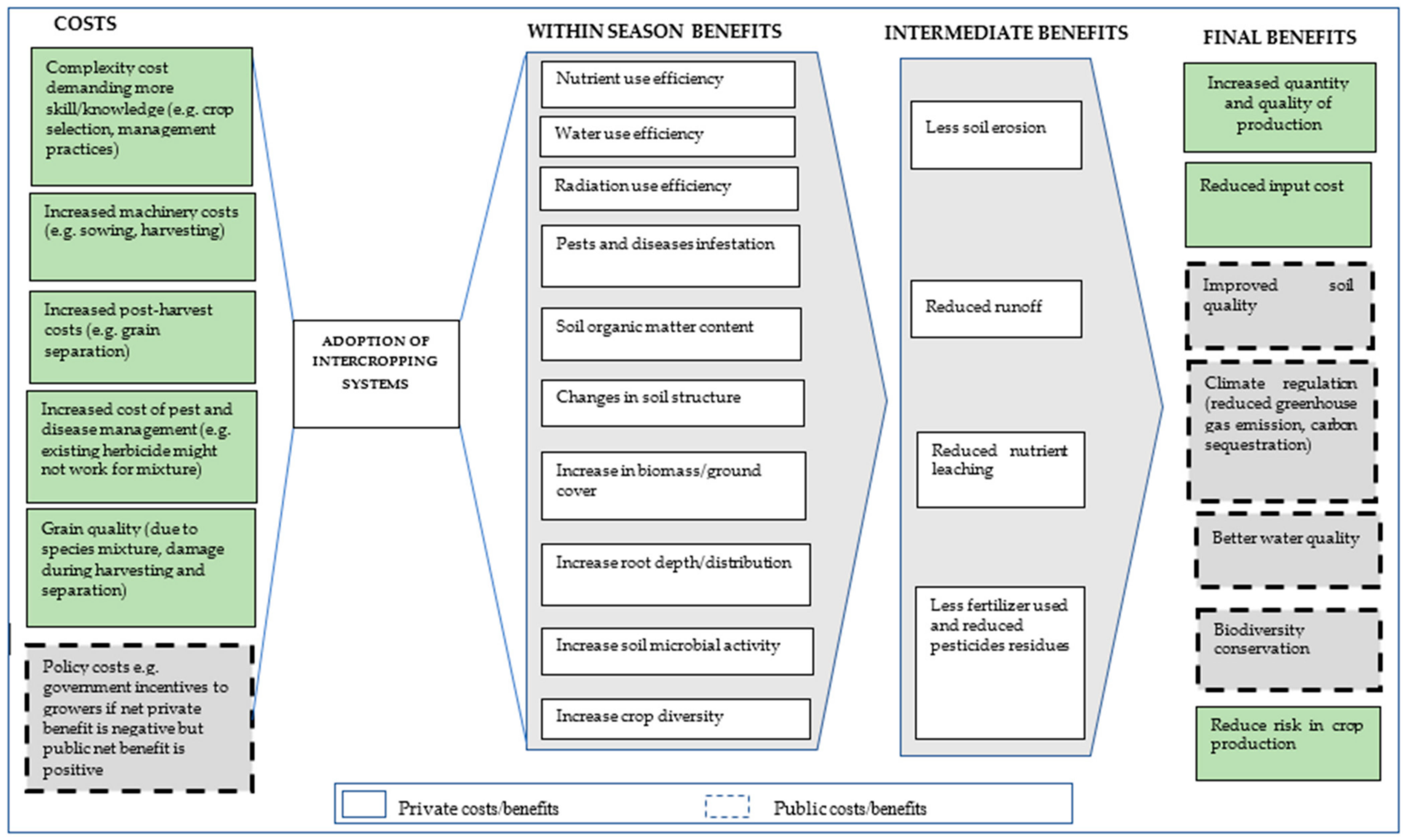
• Valuing the benefits of intercropping beyond crop yield is also necessary, which can affect the choice of cropping strategies. Thus, the researchers’ focus should not only be on increasing the biomass and yield in the short term, but also on how the adoption of intercropping can enhance environmental services and longer-term productivity improvements.
• There are management complexities associated with intercropping which could demand more skills and knowledge, change in machinery and infrastructure etc, thereby increasing the cost of producing intercrops as compared to monocrops. Evaluation of intercropping advantages should consider not only benefits but also costs associated.
• There is a need to use appropriate profit and risk metrics in assessing intercropping. We recommend the use of the net gross margin, profit ratio and the ’certainty equivalent’ that can take into account all possible private differences in costs and benefits between intercropping and monocropping systems, including the implications for business risk and the decision-makers risk tolerance.

References

1. Baulcombe, D.; Crute, I.; Davies, B.; Dunwell, J.; Gale, M.; Jones, J.; Pretty, J.; Sutherland, W.; Toulmin, C. Reaping the Benefits: Science and the Sustainable Intensification of Global Agriculture; The Royal Society: London, UK, 2009. [Google Scholar]
2. Antle, J.M.; Ray, S. Sustainable Agricultural Development An. Economic Perspective. In Palgrave Studies in Agricultural Economics and Food Policy; Christopher, B., Ed.; Cornell University: Ithaca, NY, USA, 2020; Available online: https://0-link-springer-com.brum.beds.ac.uk/book/10.1007%2F978-3-030-34599-0 (accessed on 17 February 2021).
3. Boult, C.; Chancellor, W. Productivity of Australian Broadacre and Dairy Industries, 2018–2019; Research Report; Australian Bureau of Agricultural and Resource Economics and Sciences (ABARES): Canberra, Australia, 2020. [Google Scholar]
4. O’Donnell, C. Productivity and Efficiency Analysis: An Economic Approach to Measuring and Explaining Managerial Performance; Springer Nature: Singapore, 2018. [Google Scholar]
5. Bernard, B.; Lux, A. How to feed the world sustainably: An overview of the discourse on agroecology and sustainable intensification. Reg. Environ. Chang. 2017, 17, 1279–1290. [Google Scholar] [CrossRef]
6. Barr, N. The Social Landscapes of Rural Victoria. In Landscape Analysis and Visualisation: Spatial Models for Natural Resource Management and Planning; Springer Science & Business Media: Berlin/Heidelberg, Germany, 2008; pp. 305–325. [Google Scholar] [CrossRef]
7. Eadie, L.; Stone, C.; Burton, R. Farming Smarter, not Harder: Securing Our Agricultural Economy; Centre for Policy Development: Sydney, Australia, 2012. [Google Scholar]
8. Dowling, A.; Sadras, V.O.; Roberts, P.; Doolette, A.; Zhou, Y.; Denton, M.D. Legume-oilseed intercropping in mechanised broadacre agriculture–A review. Field Crops Res. 2021, 260. [Google Scholar] [CrossRef]
9. Altieri, M.A.; Funes-Monzote, F.R.; Petersen, P. Agroecologically efficient agricultural systems for smallholder farmers: Contributions to food sovereignty. Agron. Sustain. Dev. 2012, 32, 1–13. [Google Scholar] [CrossRef] [Green Version]
10. Sullivan, P. Intercropping Principles and Production Practices. Appropriate Technology Transfer for Rural Areas Publication. 2003. Available online: http://www.attra.ncat.org (accessed on 12 January 2021).
11. Amanullah, F.K.; Muhammad, H.; Jan, A.U.; Ali, G. Land equivalent ratio, growth, yield and yield components response of mono-cropped vs. inter-cropped common bean and maize with and without compost application. Agric. Biol. J. N. Am. 2016, 7, 40–49. [Google Scholar]
12. Bedoussac, L.; Journet, E.P.; Hauggaard-Nielsen, H.; Naudin, C.; Corre-Hellou, G.; Jensen, E.S.; Prieur, L.; Justes, E. Ecological principles underlying the increase of productivity achieved by cereal-grain legume intercrops in organic farming. A review. Agron. Sustain. Dev. 2015, 35, 11–935. [Google Scholar] [CrossRef]
13. Bybee-Finley, K.; Ryan, M.R. Advancing intercropping research and practices in industrialized agricultural landscapes. Agriculture 2018, 8, 80. [Google Scholar] [CrossRef] [Green Version]
14. Tilman, D. Benefits of intensive agricultural intercropping. Nat. Plants 2020, 6, 604–605. [Google Scholar] [CrossRef]
15. De Roest, K.; Ferrari, P.; Knickel, K. Specialisation and economies of scale or diversification and economies of scope? Assessing different agricultural development pathways. J. Rural Stud. 2018, 59, 222–231. [Google Scholar] [CrossRef]
16. Cowger, C.; Weisz, R. Winter wheat blends (mixtures) produce a yield advantage in North Carolina. Agron. J. 2008, 100, 169–177. [Google Scholar] [CrossRef]
17. Kiær, L.P.; Skovgaard, I.M.; Østergård, H. Grain yield increase in cereal variety mixtures: A meta-analysis of field trials. Field Crops Res. 2009, 114, 361–373. [Google Scholar] [CrossRef]
18. Lin, B.B. Resilience in agriculture through crop diversification: Adaptive management for environmental change. BioScience 2011, 61, 183–193. [Google Scholar] [CrossRef] [Green Version]
19. Makate, C.; Wang, R.; Makate, M.; Mango, N. Crop diversification and livelihoods of smallholder farmers in Zimbabwe: Adaptive management for environmental change. SpringerPlus 2016, 5, 1135. [Google Scholar] [CrossRef] [Green Version]
20. Sharma, N.K.; Singh, R.J.; Mandal, D.; Kumar, A.; Alam, N.M.; Keesstra, S. Increasing farmer’s income and reducing soil erosion using intercropping in rainfed maize-wheat rotation of Himalaya, India. Agric. Ecosyst. Environ. 2017, 247, 43–53. [Google Scholar] [CrossRef]
21. Manevski, K.; Børgesen, C.D.; Andersen, M.N.; Kristensen, I.S. Reduced nitrogen leaching by intercropping maize with red fescue on sandy soils in North Europe: A combined field and modeling study. Plant Soil 2015, 388, 67–85. [Google Scholar] [CrossRef]
22. Gou, F.; van Ittersum, M.K.; Wang, G.; van der Putten, P.E.; van der Werf, W. Yield and yield components of wheat and maize in wheat–maize intercropping in the Netherlands. Eur. J. Agron. 2016, 76, 17–27. [Google Scholar] [CrossRef]
23. Hombegowda, H.C.; Adhikary, P.P.; Jakhar, P.; Madhu, M.; Barman, D. Hedge row intercropping impact on run-off, soil erosion, carbon sequestration and millet yield. Nutr. Cycl. Agroecosyst. 2020, 116, 103–116. [Google Scholar] [CrossRef]
24. Johnston, G.; Vaupel, S.; Kegel, F.; Cadet, M. Crop and farm diversification provide social benefits. Calif. Agric. 1995, 49, 10–16. [Google Scholar] [CrossRef] [Green Version]
25. Zhang, C.; Dong, Y.; Tang, L.; Zheng, Y.; Makowski, D.; Yu, Y.; Zhang, F.; van der Werf, W. Intercropping cereals with faba bean reduces plant disease incidence regardless of fertilizer input; a meta-analysis. Eur. J. Plant Pathol. 2019, 154, 931–942. [Google Scholar] [CrossRef]
26. Ma, Y.H.; Fu, S.L.; Zhang, X.P.; Zhao, K.; Chen, H.Y. Intercropping improves soil nutrient availability, soil enzyme activity and tea quantity and quality. Appl. Soil Ecol. 2017, 119, 171–178. [Google Scholar] [CrossRef]
27. Nyawade, S.O.; Karanja, N.N.; Gachene, C.K.; Gitari, H.I.; Schulte-Geldermann, E.; Parker, M.L. Short-term dynamics of soil organic matter fractions and microbial activity in smallholder potato-legume intercropping systems. Appl. Soil Ecol. 2019, 142, 123–135. [Google Scholar] [CrossRef]
28. Schmidt, O.; Curry, J.P.; Hackett, R.A.; Purvis, G.; Clements, R.O. Earthworm communities in conventional wheat monocropping and low-input wheat-clover intercropping systems. Ann. Appl. Biol. 2001, 138, 377–388. [Google Scholar] [CrossRef]
29. Schmidt, O.; Clements, R.; Donaldson, G. Why do cereal–legume intercrops support large earthworm populations? Appl. Soil Ecol. 2003, 22, 181–190. [Google Scholar] [CrossRef]
30. Nyawade, S.O.; Karanja, N.N.; Gachene, C.K.; Gitari, H.I.; Schulte-Geldermann, E.; Parker, M. Optimizing soil nitrogen balance in a potato cropping system through legume intercropping. Nutr. Cycl. Agroecosyst. 2020, 12, 1–7. [Google Scholar] [CrossRef] [Green Version]
31. Latati, M.; Aouiche, A.; Tellah, S.; Laribi, A.; Benlahrech, S.; Kaci, G.; Ouarem, F.; Ounane, S.M. Intercropping maize and common bean enhance microbial carbon and nitrogen availability in low phosphorus soil under Mediterranean conditions. Eur. J. Soil Biol. 2017, 80, 9–18. [Google Scholar] [CrossRef]
32. Ren, Y.Y.; Wang, X.L.; Zhang, S.Q.; Palta, J.A.; Chen, Y.L. Influence of spatial arrangement in maize-soybean intercropping on root growth and water use efficiency. Plant Soil 2017, 415, 131–144. [Google Scholar] [CrossRef]
33. Ren, J.; Zhang, L.; Duan, Y.; Zhang, J.; Evers, J.B.; Zhang, Y.; Su, Z.; van der Werf, W. Intercropping potato (Solanum tuberosum L.) with hairy vetch (Vicia villosa) increases water use efficiency in dry conditions. Field Crops Res. 2019, 240, 168–176. [Google Scholar] [CrossRef]
34. Njeru, E.M. Crop diversification: A potential strategy to mitigate food insecurity by smallholders in sub-Saharan Africa. J. Agric. Food Syst. Community Dev. 2013, 3, 63–69. [Google Scholar] [CrossRef] [Green Version]
35. Iqbal, N.; Hussain, S.; Ahmed, Z.; Yang, F.; Wang, X.; Liu, W.; Yong, T.; Du, J.; Shu, K.; Yang, W.; et al. Comparative analysis of maize–soybean strip intercropping systems: A review. Plant Prod. Sci. 2019, 22, 131–142. [Google Scholar] [CrossRef] [Green Version]
36. Mamine, F. Barriers and levers to developing wheat–pea intercropping in Europe: A review. Sustainability 2020, 12, 6962. [Google Scholar] [CrossRef]
37. Lithourgidis, A.S.; Vasilakoglou, I.B.; Dhima, K.V.; Dordas, C.A.; Yiakoulaki, M.D. Forage yield and quality of common vetch mixtures with oat and triticale in two seeding ratios. Field Crops Res. 2006, 99, 106–113. [Google Scholar] [CrossRef]
38. Swinton, S.M.; Jolejole-Foreman, C.B.; Lupi, F.; Ma, S.; Zhang, W.; Chen, H. Economic value of ecosystem services from agriculture. In The Ecology of Agricultural Landscapes: Long-Term Research on the Path to Sustainability; Hamilton, S.K., Doll, J.E., Robertson, G.P., Eds.; Oxford University Press: New York, NY, USA, 2015; pp. 54–76. [Google Scholar]
39. Willey, R.W.; Osiru, D.S.O. Studies on mixtures of maize and beans (Phaseolus vulgaris) with particular reference to plant population. J. Agric. Sci. 1972, 79, 517–529. [Google Scholar] [CrossRef]
40. Mead, R.; Willey, R.W. The concept of a ‘land equivalent ratio’and advantages in yields from intercropping. Exp. Agric. 1980, 16, 217–228. [Google Scholar] [CrossRef] [Green Version]
41. Adetiloye, P.O.; Ezedinma, F.O.C.; Okigbo, B.N. A land equivalent coefficient (LEC) concept for the evaluation of competitive and productive interactions in simple to complex crop mixtures. Ecol. Model. 1983, 19, 27–39. [Google Scholar] [CrossRef]
42. Harris, D.; Natarajan, M.; Willey, R.W. Physiological basis for yield advantage in a sorghum/groundnut intercrop exposed to drought. 1. Dry-matter production, yield, and light interception. Field Crops Res. 1987, 17, 259–272. [Google Scholar] [CrossRef] [Green Version]
43. Wilson, J.B. Shoot competition and root competition. J. Appl. Ecol. 1988, 25, 279–296. [Google Scholar] [CrossRef]
44. Odo, P.E. Evaluation of short and tall sorghum varieties in mixtures with cowpea in the Sudan savanna of Nigeria: Land equivalent ratio, grain yield and system productivity index. Exp. Agric. 1991, 27, 435–441. [Google Scholar] [CrossRef]
45. Francis, C.A. Future perspectives of multiple cropping. In Multiple Cropping Systems; Francis, C.A., Ed.; Macmillan Publishers: New York, NY, USA, 1986; pp. 351–370. [Google Scholar]
46. Vandermeer, J.H. The Ecology of Intercropping; Cambridge University Press: Cambridge, UK, 1992. [Google Scholar]
47. Soetedjo, I.N.P.; Martin, L.D. Intercropping with canola improves the productivity and sustainability of field pea. In Proceedings of the 11th Australian Agronomy Conference, Geelong, Australia, 2–6 February 2003; Available online: http://www.regional.org.au/au/asa/2003/c/4/martin.htm (accessed on 12 January 2021).
48. Jahansooz, M.R.; Yunusa, I.A.M.; Coventry, D.R.; Palmer, A.R.; Eamus, D. Radiation-and water-use associated with growth and yields of wheat and chickpea in sole and mixed crops. Eur. J. Agron. 2007, 26, 275–282. [Google Scholar] [CrossRef] [Green Version]
49. Eyre, J.X.; Routley, R.A.; Rodriguez, D.; Dimes, J.P. Intercropping maize and mungbean to intensify summer cropping systems in Queensland, Australia. In World Congress on Conservation Agriculture 2011 Papers, Proceedings of the 5th World Congress on Conservation Agriculture and Farming Systems Design, Brisbane, Australia, 26–29 September 2011; Asia-Pacific Association of Agricultural Research Institution: Bangkok, Thailand, 2011. [Google Scholar]
50. Craig, P.R. Development of a Novel Crop-Pasture System for Mixed Farms in the Higher Rainfall Zone of Southern Australia. Ph.D. Thesis, School of Agriculture, Food and Wine, The University of Adelaide, Adelaide, Australia, 2011. [Google Scholar]
51. Malhi, S.S. Improving crop yield, N uptake and economic returns by intercropping barley or canola with pea. Agric. Sci. 2012, 3. [Google Scholar] [CrossRef] [Green Version]
52. Schultz, B.; Phillips, C.; Rosset, P.; Vandermeer, J. An experiment in intercropping cucumbers and tomatoes in southern Michigan, USA. Sci. Hortic. 1982, 18, 1–8. [Google Scholar] [CrossRef]
53. Dutra, A.F.; de Melo, A.S.; Dutra, W.F.; da Silva, F.G.; de Oliveira, I.M.; Suassuna, J.F.; Neto, J.G.V. Agronomic performance and profitability of castor bean (‘Ricinus communis’ L.) and peanut (‘Arachis hypogaea’ L.) intercropping in the Brazilian semiarid region. Aust. J. Crop Sci. 2015, 9, 120. [Google Scholar]
54. Ngwira, A.R.; Aune, J.B.; Mkwinda, S. On-farm evaluation of yield and economic benefit of short-term maize legume intercropping systems under conservation agriculture in Malawi. Field Crops Res. 2012, 132, 149–157. [Google Scholar] [CrossRef]
55. Azam-Ali, S.N.; Matthews, R.B.; Williams, J.H.; Peacock, J.M. Light use, water uptake and performance of individual components of a sorghum/groundnut intercrop. Exp. Agric. 1990, 26, 413–427. [Google Scholar] [CrossRef]
56. Choudhary, V.K.; Dixit, A.; Chauhan, B.S. Resource-use maximisation through legume intercropping with maize in the eastern Himalayan region of India. Crop. Pasture Sci 2016, 67, 508–519. [Google Scholar] [CrossRef]
57. Wang, Z.G.; Jin, X.; Bao, X.G.; Li, X.F.; Zhao, J.H.; Sun, J.H.; Christie, P.; Li, L. Intercropping enhances productivity and maintains the most soil fertility properties relative to sole cropping. PLoS ONE 2014, 9, e113984. [Google Scholar] [CrossRef] [Green Version]
58. Lithourgidis, A.S.; Vlachostergios, D.N.; Dordas, C.A.; Damalas, C.A. Dry matter yield, nitrogen content, and competition in pea–cereal intercropping systems. Eur. J. Agron. 2011, 34, 287–294. [Google Scholar] [CrossRef]
59. Pelzer, E.; Bazot, M.; Makowski, D.; Corre-Hellou, G.; Naudin, C.; Al Rifaï, M.; Carrouée, B. Pea–wheat intercrops in low-input conditions combine high economic performances and low environmental impacts. Eur. J. Agron. 2012, 40, 39–53. [Google Scholar] [CrossRef]
60. Kermah, M.; Franke, A.C.; Adjei-Nsiah, S.; Ahiabor, B.D.; Abaidoo, R.C.; Giller, K.E. Maize-grain legume intercropping for enhanced resource use efficiency and crop productivity in the Guinea savanna of northern Ghana. Field Crops Res. 2017, 213, 38–50. [Google Scholar] [CrossRef]
61. Huang, C.; Liu, Q.; Heerink, N.; Stomph, T.; Li, B.; Liu, R.; van der Werf, W. Economic performance and sustainability of a novel intercropping system on the North China Plain. PLoS ONE 2015, 10, e0135518. [Google Scholar] [CrossRef] [Green Version]
62. Li, Q.Z.; Sun, J.H.; Wei, X.J.; Christie, P.; Zhang, F.S.; Li, L. Overyielding and interspecific interactions mediated by nitrogen fertilization in strip intercropping of maize with faba bean, wheat and barley. Plant Soil 2011, 339, 147–161. [Google Scholar] [CrossRef] [Green Version]
63. Chai, Q.; Qin, A.; Gan, Y.; Yu, A. Higher yield and lower carbon emission by intercropping maize with rape, pea, and wheat in arid irrigation areas. Agron. Sustain. Dev. 2014, 34, 535–543. [Google Scholar] [CrossRef]
64. Moghbeli, T.; Bolandnazar, S.; Panahande, J.; Raei, Y. Evaluation of yield and its components on onion and fenugreek intercropping ratios in different planting densities. J. Clean. Prod. 2019, 213, 634–641. [Google Scholar] [CrossRef]
65. Oyejola, B.A.; Mead, R. Statistical assessment of different ways of calculating land equivalent ratios (LER). Exp. Agric. 1982, 18, 125–138. [Google Scholar] [CrossRef] [Green Version]
66. Davidson, B.R.; Martin, B.R. The relationship between yields on farms and in experiments. Aust. J. Agric. Econ. 1965, 9, 129–140. [Google Scholar] [CrossRef] [Green Version]
67. Jolliffe, P.A.; Wanjau, F.M. Competition and productivity in crop mixtures: Some properties of productive intercrops. J. Agric. Sci. 1999, 132, 425–435. [Google Scholar] [CrossRef]
68. Trapnell, L.; Malcolm, L.R. Expected benefits on and off farm from including lucerne (Medicago sativa) in crop rotations on the Broken Plains of north-eastern Victoria. AFBM J. 2014, 11, 19–31. [Google Scholar]
69. Dillon, J.L. The definition of farm management. J. Agric. Econ. 1980, 31, 257–258. [Google Scholar] [CrossRef]
70. Anderson, J.R.; Dillon, J.L.; Hardaker, J.B. Agricultural Decision Analysis; Iowa State University Press: Ames, Iowa, 1977. [Google Scholar]
71. Boehlje, M.D.; Eidman, V.R. Farm Management; John Wiley and Sons: Hoboken, NJ, USA, 1984. [Google Scholar]
72. Malcolm, L.R.; Makeham, J.P.; Wright, V. The Farming Game: Agricultural Management and Marketing; Cambridge University Press: Melbourne, Australia, 2005. [Google Scholar]
73. Pannell, D. Economic perspectives on nitrogen in farming systems: Managing trade-offs between production, risk and the environment. Soil Res. 2017, 55, 473–478. [Google Scholar] [CrossRef]
74. Hadar, J.; Russell, W.R. Rules for ordering uncertain prospects. Am. Econ. Rev. 1969, 4, 25–34. [Google Scholar]
75. Hanoch, G.; Levy, H. Efficiency analysis of choices involving risk. Rev. Econ. Stud. 1969, 36, 335–345. [Google Scholar] [CrossRef]
76. Hochman, Z.; Horan, H.; Garcia, J.N.; Hopwood, G.; Whish, J.; Bell, L.; Zhang, X.; Jing, H. Cropping system yield gaps can be narrowed with more optimal rotations in dryland subtropical Australia. Agric. Syst. 2020, 184, 1–9. [Google Scholar] [CrossRef]
77. Hardaker, J.B.; Richardson, J.W.; Lien, G.; Schumann, K.D. Stochastic efficiency analysis with risk aversion bounds: A simplified approach. Aust. J. Agric. Resour. Econ. 2004, 48, 253–270. [Google Scholar] [CrossRef] [Green Version]
78. Hardaker, J.B.; Lien, G.; Anderson, J.R.; Huirne, R.B.M. Coping with Risk in Agriculture: Applied Decision Analysis, 3rd ed.; CABI Publishing: Boston, MA, USA, 2015. [Google Scholar]
79. Gandorfer, M.; Pannell, D.; Meyer-Aurich, A. Analysing the effects of risk and uncertainty on optimal tillage and nitrogen fertilizer intensity for field crops in Germany. Agric. Syst. 2011, 104, 615–622. [Google Scholar] [CrossRef]
80. Monjardino, M.; Hochman, Z.; Horan, H. Yield potential determines Australian wheat growers’ capacity to close yield gaps while mitigating economic risk. Agron. Sustain. Dev. 2019, 39, 39–49. [Google Scholar]
81. Fathelrahman, E.M.; Ascough, J.C.; Hoag, D.L.; Malone, R.W.; Heilman, P.; Wiles, L.J.; Kanwar, R.S. Economic and stochastic efficiency comparison of experimental tillage systems in corn and soybean under risk. Exp. Agric. 2011, 47, 111–136. [Google Scholar] [CrossRef] [Green Version]
82. Alcon, F.; Marín-Miñano, C.; Zabala, J.A.; de-Miguel, M.D.; Martínez-Paz, J.M. Valuing diversification benefits through intercropping in Mediterranean agroecosystems: A choice experiment approach. Ecol. Econ. 2020, 171, 106593. [Google Scholar] [CrossRef]
83. Martin-Guay, M.O.; Paquette, A.; Dupras, J.; Rivest, D. The new green revolution: Sustainable intensification of agriculture by intercropping. Sci. Total Environ. 2018, 615, 767–772. [Google Scholar] [CrossRef]
84. Cooper, J.C.; Signorello, G. Farmer premiums for the voluntary adoption of conservation plans. J. Environ. Plan. Manag. 2008, 51, 1–14. [Google Scholar] [CrossRef] [Green Version]
85. DAWE. Agriculture Stewardship Package. Department of Agriculture, Water and Environment, Australian Government, 2021. Available online: https://www.agriculture.gov.au/sites/default/files/documents/ag-steward-program-factsheet-1.pdf (accessed on 9 April 2021).
86. Willey, R. Evaluation and presentation of intercropping advantages. Exp. Agric. 1985, 21, 119–133. [Google Scholar] [CrossRef] [Green Version]
Figure 1. Typical expected costs and potential benefits of adopting intercropping systems.
Agriculture 11 00453 g001