
Impacts of Background Removal on Convolutional Neural Networks for Plant Disease Classification In-Situ


School of Electronics and Information Engineering, Harbin Institute of Technology, Harbin 150001, China
*
Author to whom correspondence should be addressed.
Agriculture 2021, 11(9), 827; https://0-doi-org.brum.beds.ac.uk/10.3390/agriculture11090827
Submission received: 15 August 2021
/
Revised: 26 August 2021
/
Accepted: 26 August 2021
/
Published: 30 August 2021
(This article belongs to the Special Issue Latest Advances for Smart and Sustainable Agriculture)
Abstract
:Convolutional neural networks have an immense impact on computer vision tasks. However, the accuracy of convolutional neural networks on a dataset is tremendously affected when images within the dataset highly vary. Test images of plant leaves are usually taken in situ. These images, apart from the region of interest, contain unwanted parts of plants, soil, rocks, and/or human body parts. Segmentation helps isolate the target region and a deep convolutional neural network classifies images precisely. Therefore, we combined edge and morphological based segmentation, background subtraction, and the convolutional neural network to help improve accuracy on image sets with images containing clean and cluttered backgrounds. In the proposed system, segmentation was applied to first extract leaf images in the foreground. Several images contained a leaf of interest interposed between unfavorable foregrounds and backgrounds. Background subtraction was implemented to remove the foreground image followed by segmentation to obtain the region of interest. Finally, the images were classified by a pre-trained classification network. The experimental results on two, four, and eight classes of datasets show that the proposed method achieves 98.7%, 96.7%, and 93.57% accuracy by fine-tuned DenseNet121, InceptionV3, and DenseNet121 models, respectively, on a clean dataset. For two class datasets, the accuracy obtained was about 12% higher for a dataset with images taken in the homogeneous background compared to that of a dataset with testing images with a cluttered background. Results also suggest that image sets with clean backgrounds tend to start training with higher accuracy and converge faster.
1. Introduction
Deep learning is a sub-field of machine learning that uses a multi-layered artificial neural network, inspired by the structure and function of the brain for learning patterns to deliver state-of-the-art accuracy. As shown in Figure 1, a biological neuron mainly comprises of dendrites, soma, or nucleus, and axon or axon terminals, which act as input activation functions and outputs, respectively, in an artificial neural network. Deep learning algorithms have significantly outperformed traditional methods in signal, image, video, speech, and text processing tasks. Convolutional neural network (CNN) is a form of an artificial neural network popularly implemented in image and video processing tasks due to its robustness and generalization abilities, which are achieved on account of deep architectures [1]. Deep CNN architectures have proven to be efficient, but require large computational and training resources [2]. CNNs demand a plethora of training data and may result in overfitting or the inability to converge when faced with insufficient data. Data augmentation, which artificially increases the amount of data within a dataset, helps tackle this problem [3]. CNNs have demonstrated exceptional results in computer vision tasks irrespective of image types in different applications, such as medical images [4,5], satellite images [6,7], or hyperspectral images [8,9].
Image noise has been a primary concern in computer vision tasks. The presence of image noise, in form of a redundant background, crucially affects the outcome of image analysis [10]. CNNs, at the cost of resources, efficiently classify images that may be affected when the region of interest is significantly smaller. Noisy data impose such a problem. The presence of unwanted objects, besides an area of interest, is considered as background noise, which drastically affects the efficacy of CNNs. Early detection of plant disease is crucial for sustainable agriculture by enhancing crop productivity. The application of image processing algorithms and deep learning models hold a significant premise in the identification and classification of plant diseases that occur due to pathogens infested in leaves or plant parts, by providing diagnostic results for the early detection of plant diseases. However, the presence of redundant and noisy backgrounds in leaf images have hindered classification accuracy. Image segmentation in conjunction with background subtraction helps increase classification accuracy. Image segmentation separates or groups an image into different parts, which finally isolates the region of interest. The segmentation process is based on various features, such as color or boundaries [11]. Background subtraction (BGS) is widely used for identifying foreground objects. The primary concept behind BGS is to detect foreground objects from the difference between the frame of interest and the reference frame, often called the background image [12].
As mentioned earlier, CNNs require an abundance of data. However, transfer learning enables CNNs to learn with limited data by transferring knowledge from models pre-trained on large datasets [13]. Transfer learning takes a source network i.e., a pre-trained model on a specific task with a larger dataset and then re-purposes it to perform on a similar target problem, usually with minimum training resources, on a small dataset [14,15]. For different sources or target domains or tasks, transfer learning emphasizes on improving the learning of predictive functions in the target domain, for better results, by applying collective knowledge from both of the domains. In transfer learning, models pre-trained on standard datasets effectively adapt to downstream tasks [16]. Transfer learning essentially extracts reusable features from earlier layers of a pre-trained network, previously trained on a larger and easily available dataset and a different task, and finally inputs those features to train a much smaller model with fewer parameters. This smaller network only needs to learn the relations for the specific problem, having already learnt about patterns in the data from the pre-trained model. Transfer learning virtually creates a shallow network within a deep network by utilizing previously learned knowledge. The process of transfer learning is accomplished either by reusing features from the second to last layer (i.e., the layer before classification layer), which is termed as feature extraction, or by fine-tuning the model for better performance.
Our work primarily focuses on increasing the classification accuracy of diseased plants on a classification problem where training and testing data visually vary. This experiment explores the limitation imposed by Mohanty et al. [17], where it is mentioned that a real world application should be able to classify images of a disease, as it presents itself directly on the plant, i.e., testing the image in field conditions. It is shown that CNNs are prone to decreased efficiency, while working with test data, which have a high variance to training data. Models trained on images with clean backgrounds or images taken on laboratory conditions fail to achieve higher accuracy when tested with images with cluttered backgrounds or taken on field conditions. Testing the transfer learned models on pre-processed images (pre-processed using image segmentation and background removal to remove the background) provide a significant boost to classification accuracy.
1.1. Related Works
Early and accurate detection and classification of plant diseases are of utmost importance to increase crop yield. Numerous research studies have been conducted to increase plant disease identification accuracy and decrease food loss. Automatic detection of plant disease was conducted by implementing four steps viz. color transformation, masking of green pixels, and removal using specific threshold, segmentation by creating equal sized patches, and employing a classifier on a database of 500 plants [18]. A combination of a genetic algorithm to obtain useful segments and a support vector machine (SVM) classifier was used to classify plant diseases [19]. Various image segmentation techniques, such as a difference of pixel values between neighborhood pixels and k-means based segmentation, were employed to identify plant disease with 93% accuracy [20]. Most research on the segmentation of plant leaves have focused on lesion isolation.
While image segmentation has been used for image identification and classification of plant leaves, few studies have focused on background removal of plant leaf images. Wang et al. present an effective image segmentation method based on the Chan–Vese model and Sobel operator. This method consists of three stages: a feature that identifies hues with relatively high levels of green were used to extract the region of leaves and remove the background, the Chan–Vese model and improved Sobel operator were implemented to extract the leaf contours and detect the edges, respectively, and a target leaf with a complex background and overlapping was extracted by combining the results obtained by the Chan–Vese model and Sobel operator [21]. Chen et al. proposed an enhanced segmentation method to remove shadows for vehicle detection [22]. Background estimation and noise removal from the retinal image was performed by applying coarse and fine segmentation for automated diagnosis of diabetic retinopathy, which significantly improved the accuracy [23].
CNNs outperformed the fully connected multilayer perceptron (MLP) by yielding 85% accuracy on major crops, such as wheat, maize, sunflower, soybean, sugar beet, etc., while classifying crops from remote sensing (RS) images acquired by Landsat-8 and Sentinel-1A RS satellites [24]. Depth-wise separable convolutional neural networks suitable for mobile applications were employed to classify 55 classes and 82,161 plant disease leaf RGB images with 98.34% accuracy [25]. Various state-of-the-art CNN models, pre-trained on ImageNet [26], were re-trained to classify leaf images from 28 classes incorporating 15 crop species, and a total of 23,352 images to achieve an accuracy of 99.74% [27]. INC-VGGN achieved an accuracy of 92% on rice disease images under complex background conditions. This model combined a pre-trained VGG model with an inception module to combine the advantages of both inception and VGGNet [28]. Transfer learning was applied to a pre-trained CNN (GoogLeNet) to classify 12 plant species with 1383 images and 56 classes. This model achieved an accuracy of 84% for image sets with original images and 87% accuracy with background-removed image sets [29].
1.2. Problems with a Cluttered Background
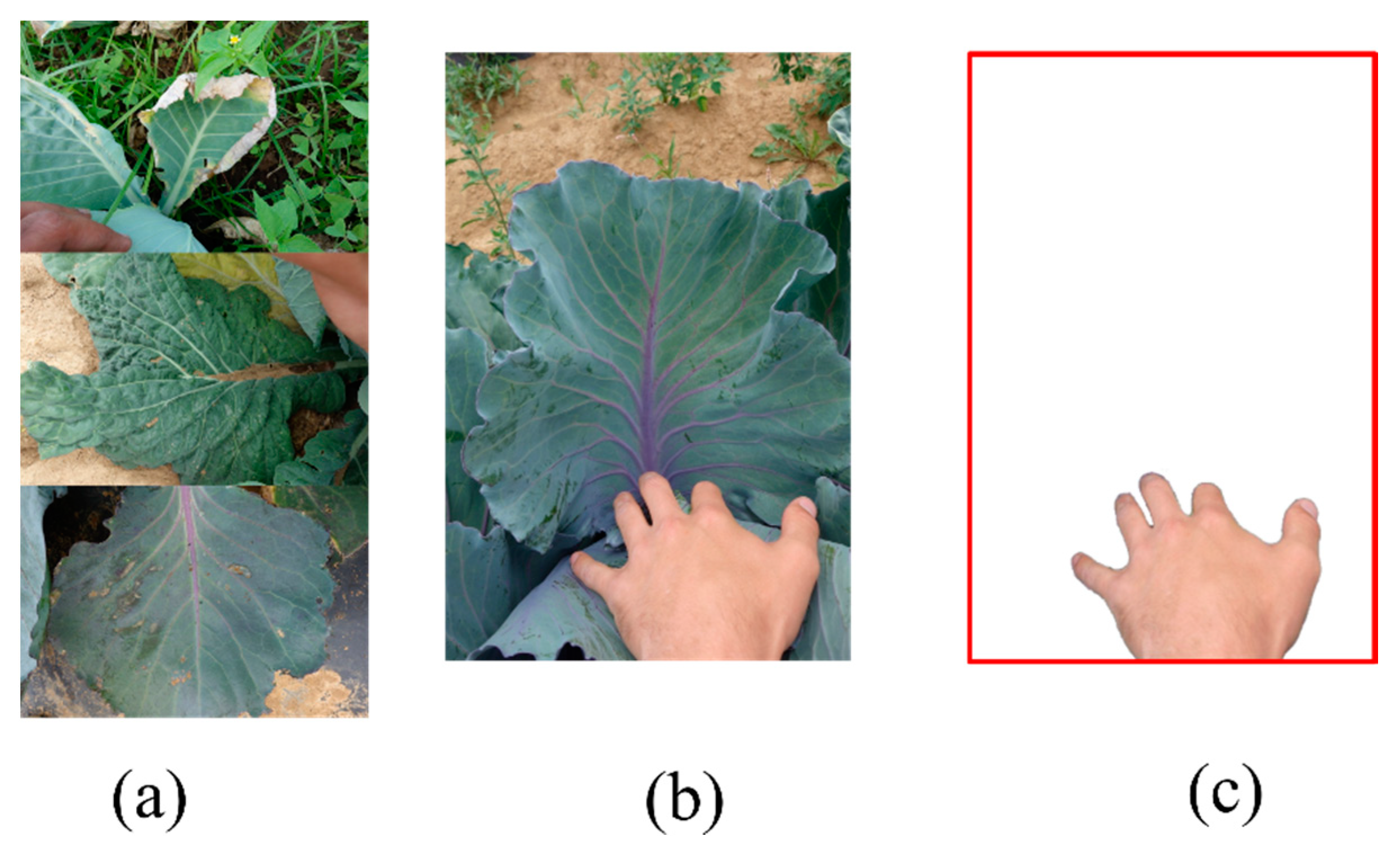
The major problem with images in situ is the presence of undesired subjects in the image. This issue can be seen in a plant leaf, in the form of mud on top of a healthy leaf image, or a leaf from another plant on top of the desired leaf image, as shown in Figure 2a, or the appearance of a human body part in the foreground of the leaf image, as seen in Figure 2b. When a segmentation algorithm is applied for background removal on such images, the region of interest could be considered as background, and removed, as shown in Figure 2c. Thus, simply using segmentation is not suitable for certain images in the image set, and requires additional processing. Applying the background subtraction algorithm after segmentation helps create the image with the area of interest on the foreground with undesirable objects in the background. Reiterating the segmentation process helps to correctly remove the background from the input image.
2. Materials and Methods
2.1. Proposed Approach
We propose an automatic and intelligent method for classifying plant diseases based on leaf images under true field conditions. Since most of the research focuses on isolating the lesion instead of isolating the leaf from the image, we implemented algorithms to isolate the leaf from an image containing noisy background. The classification system is a combination of edge-based segmentation, background subtraction, and transfer learning of the convolutional neural network. Figure 3 shows the framework of the proposed method, including the training and testing phases. In the initial phases, the input frame is processed by applying edge-based segmentation in junction with morphological segmentation to extract objects of interest in the foreground. When the region of interest is interposed between two unwanted objects, background subtraction is implemented to remove the foreground object, followed by segmentation to obtain the object of interest from the input image. During the final phases, these images are fed to pre-trained convolutional neural network models. Fine-tuned models pre-trained on the ImageNet dataset were utilized for the classification of plant diseases.
2.2. Edge and Morphological Based Segmentation
Image segmentation is defined as the process of distinguishing different objects within an image. This includes separating objects from their background. The main idea of image segmentation is to separate leaves of interest from the noisy background that contains plant parts, human body parts, soil etc. Edge detection is a technique in which the point where sharp changes in image properties are identified and organized using line segments to form edges. Canny edge detection is a non-maximum suppression technique based on a Gaussian filter. Canny edge takes the output from the Sobel operator and thins all the edges followed by hysteresis thresholding. Steps involved in the canny edge detection algorithm are shown in Algorithm 1.
| Algorithm 1. Canny edge detection algorithm |
|
Morphological filters are a collection of non-linear operations carried out relatively on the ordering of pixels, without affecting their numerical value. Erosion and dilation are two fundamental operators in morphological filters. Erosion replaces the current pixel value with the minimum value found in a defined set of pixels. Dilation replaces the current pixel value with the maximum value found in a defined set of pixels [30]. Combining canny edge detection and morphological operations results in a background removal algorithm, as in Algorithm 2. The threshold values were taken from a range depending on the outcome of the image.
, , , , were the values used.
| Algorithm 2. Algorithm for Background Removal |
|
2.3. Background Subtraction
Background subtraction (BGS) has been extensively used in video processing where successive frames are used to detect foreground objects [31]. However, this concept can be utilized to remove foreground objects if the foreground objects are not the region of interest.
For an input image and background , the foreground image is given as where, is a threshold value. Similarly, the background can be obtained by subtracting foreground from image i.e., . Figure 4 shows the removal of the human hand present in the foreground by applying BGS on the input image and the background removed image after applying the segmentation algorithm.
2.4. Transfer Learning and Fine-Tuning
Transfer learning is employed when the training dataset has a smaller amount of data and is similar to a pre-trained dataset. Transfer learning is carried out by (i) creating a suitable network by stacking neural layers, training the neural network on a dataset with abundant data, and finally fine-tuning the network on the available dataset; or by (ii) reusing state-of-the-art model pre-trained on a standard dataset with surfeit and analogous data, and fine-tuning in correspondence to available data. The latter is favored as this reduces the inconvenience of creating a model and saves time for training on a different set of data. Given a source domain , where is a feature space and is a marginal probability distribution in which , source task , where is label space and an objective predictive function, target domain , where is a feature space and is a marginal probability distribution in which and target task , where is label space and an objective predictive function, such that . Predictive function is learned from source training data, which consists of pairs and is learned from target training data, which consists of pairs in junction with . While classifying diseased plant leaf images based on ImageNet dataset, the source task and the target task are different (i.e., ). The label spaces between these two tasks are different (i.e., ). Inductive transfer learning is proven to be the best solution to solve such problems. In inductive transfer learning, the common features can be learned by solving an optimization problem [14], given as
In this equation, and denote the tasks in the source domain and target domain, respectively. is a matrix of parameters. U is a orthogonal matrix (mapping function) for mapping the original high-dimensional data to low-dimensional representations. The -norm of is defined as The optimization problem (4) estimates the low-dimensional representations , and the parameters, of the model at the same time.
Transfer learning makes use of previously learned knowledge on new tasks. Reusable features extracted by models pre-trained on ImageNet was applied to re-train the model on the plant leaf dataset. Transfer learning of a model is generally conducted in two ways: the model used as a feature extractor and fine-tuning the model. These models are state-of-the-art models, such as VGG19 [32], ResNet [33], Inception [34], MobileNet [35], MobilenetV2 [36], DenseNet [37], NA SNetMobile [38], etc. Transfer learning works on the concept of layer freeze. The core idea of layer freeze is not to update the layer weights while training on a new dataset to obviate making changes on formerly extracted reusable features generated by filters in earlier layers. Depending on the frozen layers, parameters are divided into non-trainable parameters and trainable parameters. The former corresponds to parameters of frozen layers whereas, the network trains on remaining parameters corresponding to layers that are not frozen. In contrast to the back propagating and updating the weights of all the layers in the network, fine-tuning drastically reduces the computational cost. There is an inverse relationship between the number of frozen layers and the number of trainable parameters. Feature extractor is employed by replacing the final output layer with the suitable classifier and freezing the weight for whole network excluding the final fully connected layer, whose neurons have full connections to all activations in the previous layer. The rest of the network is treated as a fixed feature extractor while the reusable features are entirely extracted from ImageNet. In fine-tuning, not only the classifier is replaced, but the weights of the pre trained network is also fine-tuned by continuing the backpropagation. The number of layers required to fine-tune depends upon the data used and the type of network. While fine-tuning all of the layers of the model could be re-trained, it is preferred to keep few earlier layers frozen to avoid overfitting, and only fine-tine some higher-level layers of the network. We opted for fine-tuning instead of feature extractor for higher accuracy in expense of slightly higher computational costs [27].
2.5. Convolutional Block
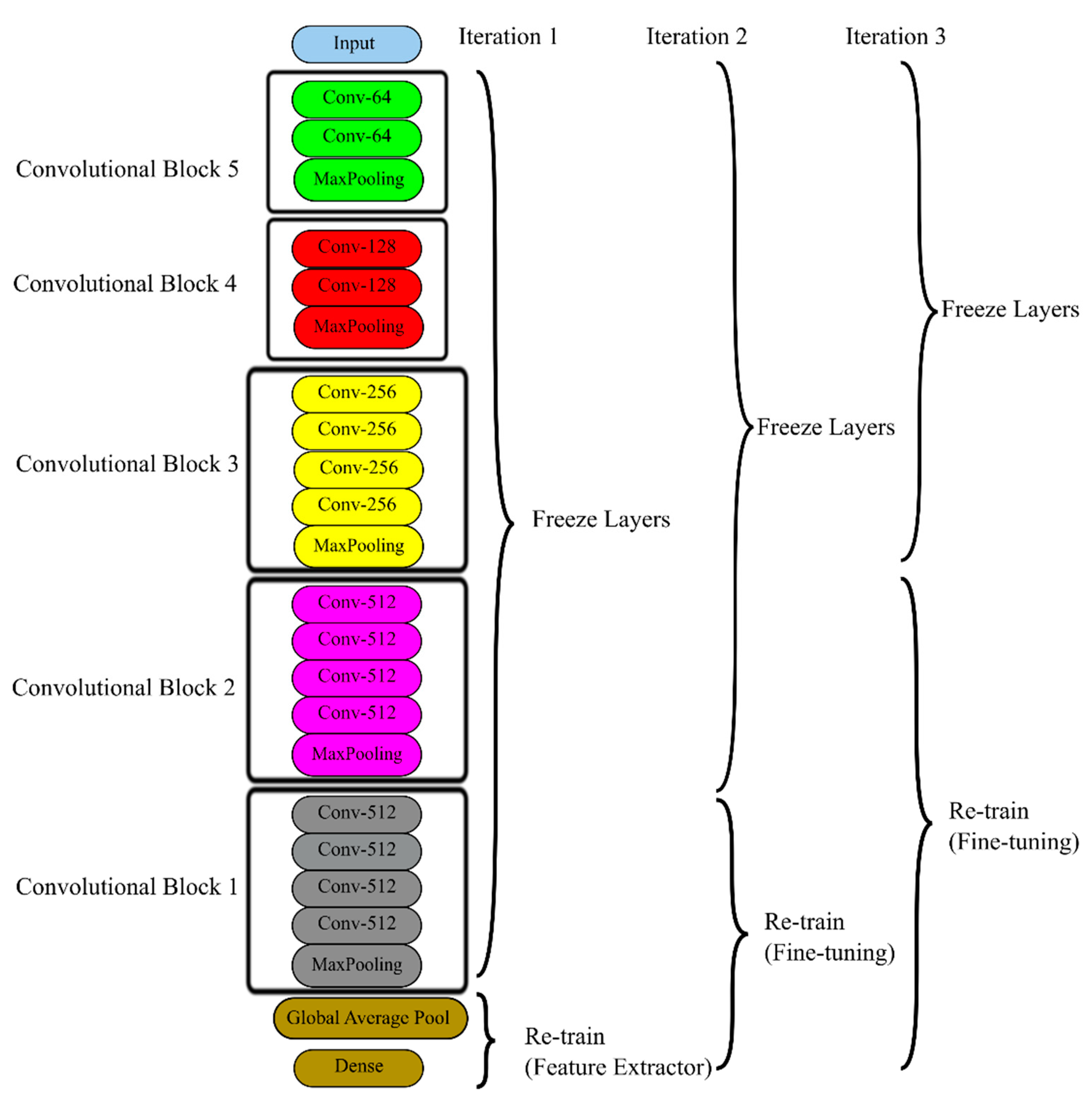
A convolutional block is referred to as a collection of layers in a model comprising of a convolutional layer and all the layers before the succeeding convolutional layer, or a group of convolutional layers together with other layers, depending on the model architecture. Convolutional blocks are unfrozen and frozen instead of individual layers, which helps to reach the desired accuracy faster. Trainable blocks are the convolutional blocks that are not being frozen. Figure 5 shows the convolutional blocks and fine-tuning process for the VGG19 model. Trainable parameters are the total number of parameters that get re-trained on the new data. Thus, while fine-tuning, freezing and unfreezing blocks are efficient, compared to individual layers. It is preferred to re-train the model with lesser layers as training time significantly reduces compared to training the whole model. As shown in Figure 5, while fewer layers, and then more layers to obtain the desired result, using convolutional blocks and suitable hyperparameters, help achieve higher accuracy faster.
The Nadam optimization algorithm was used. Real-time augmentation was adopted for data augmentation, which generates batches of augmented data while the model is still training. This saves overhead memory on top of making the model robust. Hyper-parameters and data augmentations used are listed in Table 1.
2.6. Dataset
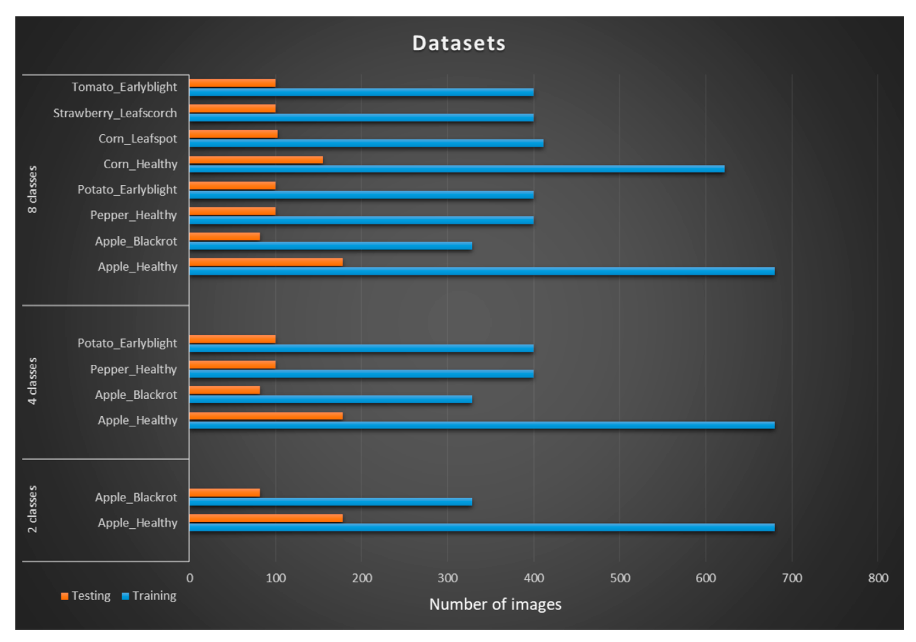
The plant leaf dataset used in the experiment was taken from the PlantVillage dataset [39]. The images in the PlantVillage dataset were taken from various plants with and without diseases. While most of the images were of a single leaf taken with homogeneous background, a certain amount of images were taken in field condition. The dataset in our experiment is a subset of the PlantVillage dataset and is divided into three datasets of two, four, and eight. Each class contains images with a clean and cluttered background. Images with clean backgrounds were used for training and images with cluttered backgrounds for testing. These datasets are labeled as dataset1a, dataset2a and dataset3a for two, four, and eight classes, respectively. Different datasets were created by cleaning cluttered images. These datasets are labeled as dataset1b, dataset2b and dataset3b for two, four, and eight, respectively. Figure 6 shows the classes information of the dataset. A total of 4588 images from eight classes and six plant species were used for the experiment. Dataset1a and dataset1b contain 1268 images from two classes (Apple_healthy and Apple_blackrot). Similarly, dataset2(a,b) and dataset3(a,b) contains 2268 and 4558 images, respectively. Images in datasets are of varied sizes and different backgrounds. Clean images are taken in laboratory conditions where a single leaf is placed on a homogenous background and the image is taken. Cluttered images, on the other hand, are taken in situ, and comprised of a cluster of leaves along with stems, branches, and human body parts.
Dataset4a contains 484 cabbage leaf images from two classes (cabbage_healthy and cabbage_blackrot). This dataset contains all leaf images from the cabbage plants with a cluttered background. This dataset comprises of 388 images for training and 96 images for testing both with a cluttered background. Dataset4b contains the same images, but the images are cleaned using a background removal algorithm before training and testing the algorithm i.e., both training and testing images are cleaned. Training and testing images were divided into an 80:20 ratio for better results [17].
3. Results and Discussion
3.1. Background Removal
The input image was segmented into foreground and background by a combination of edge segmentation and morphological operations, and the background was converted to white background. Outputs of each operation involved in background removal can be seen in Figure 7.
The segmentation algorithm produced exemplary results on images with ample depth between foreground object and background as in Figure 8. However, the object of interest was difficult to isolate on images with complex background and foreground. Application of background subtraction followed by the segmentation algorithm on such images produced satisfactory results. Few images required manual intervention to remove background and the isolate leaf of interest.
3.2. Grad-CAM Class Activation Visualization
While CNNs have enabled superior performance, they lack interpretability. This makes models less transparent and difficult to explain the usability of components of the model. To overcome this downside, a technique called gradient-weighted class activation mapping (Grad-CAM) was introduced for producing visual explanations to make the model transparent. Grad-CAM uses the gradients of any target concept, flowing into the final convolutional layer to produce a coarse localization map highlighting important regions in the image for predicting the concept [40]. This enables the visualization of the outcome from different layers in a CNN model. The visual output of two CNN models, InceptionV3 and VGG19, is shown in Figure 9.
The first and third rows show the heat maps and superimposed image of input images, which are a healthy apple leaf image and strawberry with leaf scorch taken in field conditions, respectively. It is evident from the heatmaps and superimposed images obtained from both InceptionV3 and VGG19 models that images with backgrounds fail to extract the essential features. However, the cleaned images of the aforementioned leaf images, as seen in the second and fourth rows, have a fine localized region of interest in the image, proving that CNNs work better with cleaned images.
3.3. Classification
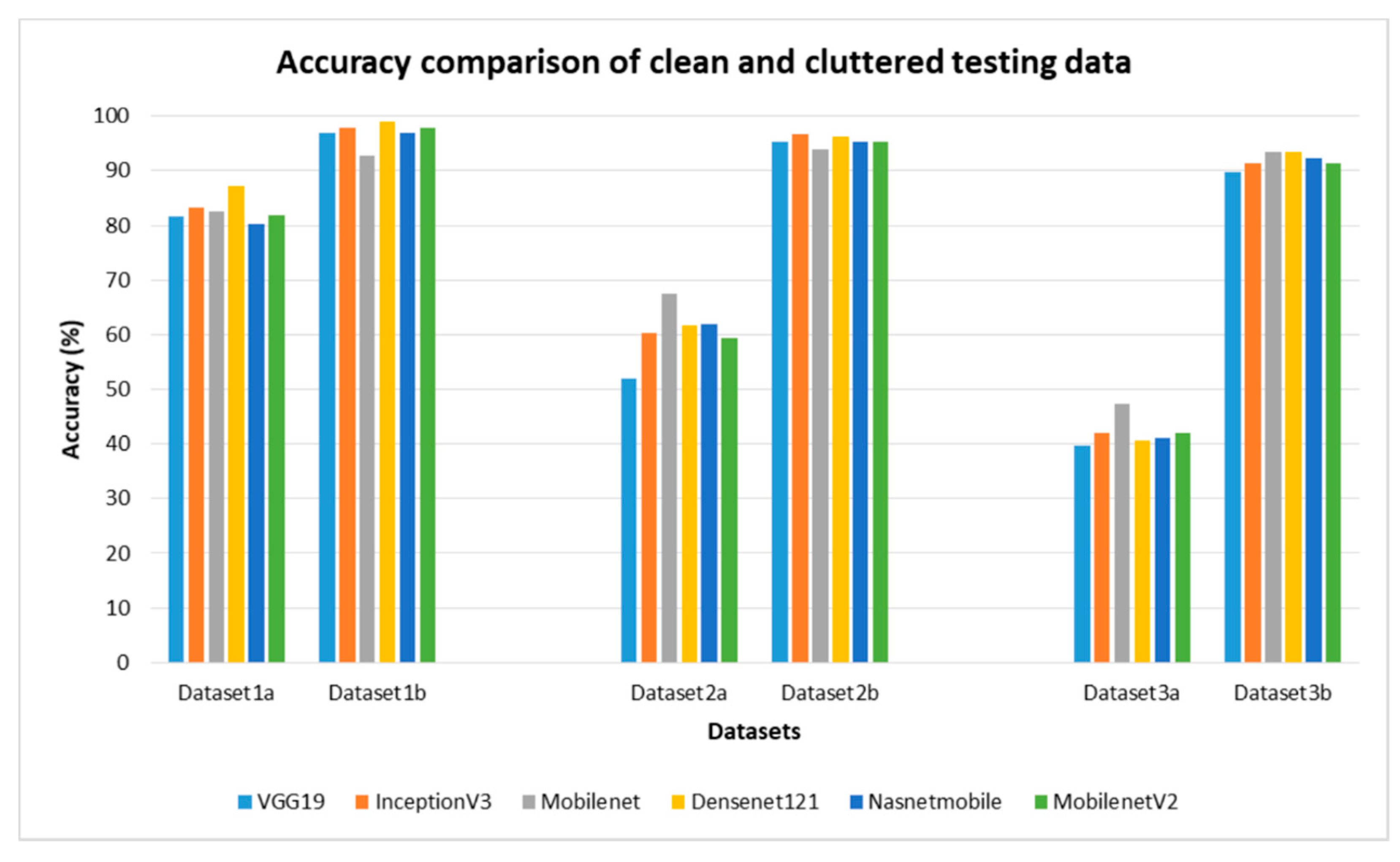
Fine-tuned DenseNet121 outperformed other fine-tuned models by achieving a test accuracy of 98.9% and 93.5% on the two-class and eight-class clean datasets whereas, fine-tuned InceptionV3 outperformed others for the four-class dataset by attaining accuracy of 96.7%. Figure 10 shows accuracies attained by various fine-tuned models on different datasets. The accuracy difference between the same models on cluttered and cleaned testing data can be seen in the figure below. Notation “a” denotes an image set with cluttered testing images and notation b denotes an image set with cleaned testing images. On dataset1, the difference in accuracy between cluttered and clean datasets (i.e., dataset1a and dataset1b) ranges from 10% for MobileNet to 16% for NA SNetMobile. For dataset2a and 3a, the highest accuracy obtained was 67.6% and 47.3%, respectively, by fine-tuned MobileNet.
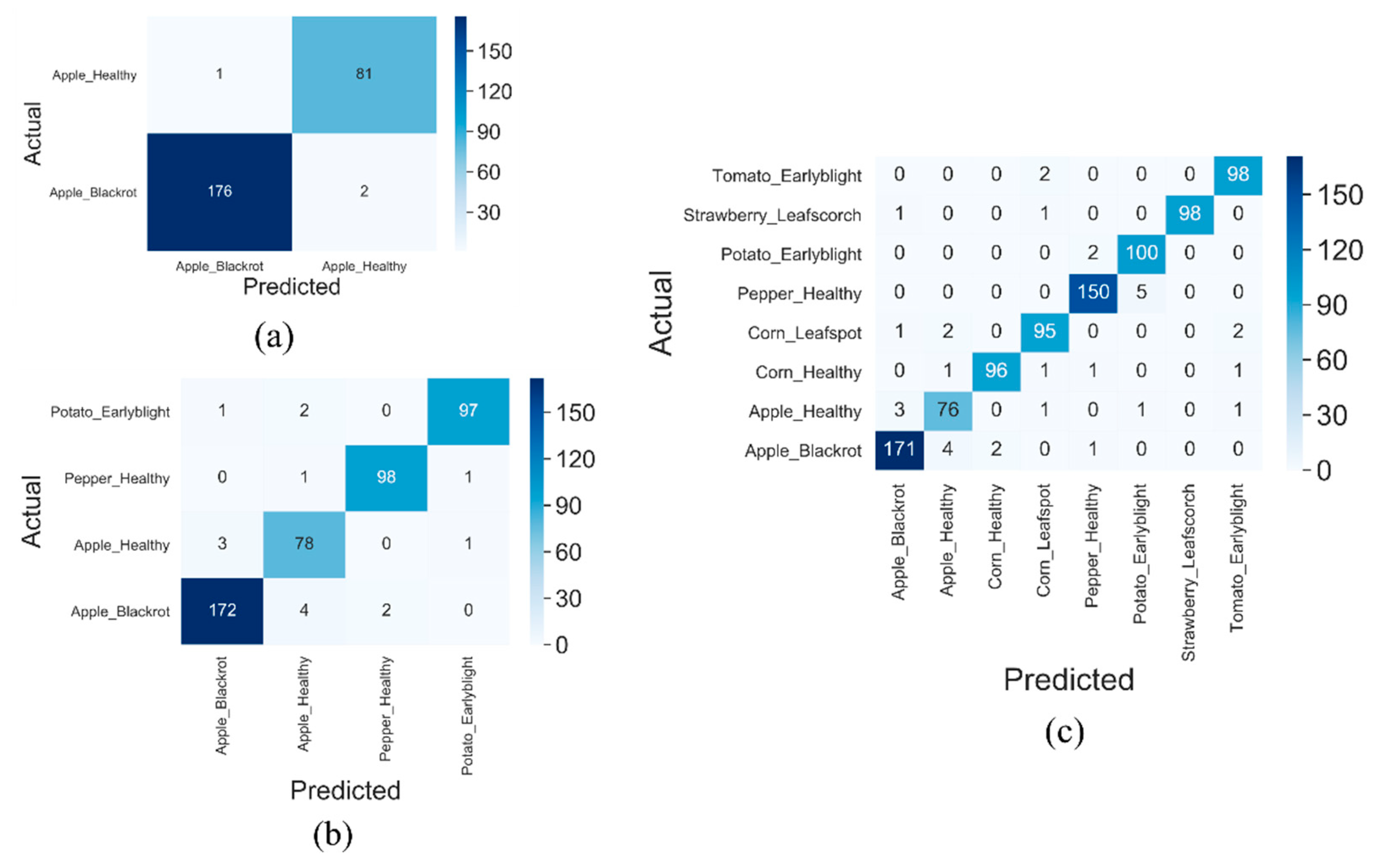
Table 2 shows the performance indicators obtained by the highest performing fine-tuned model on each dataset with a homogeneous background. DenseNet121 attained an F1-score of 0.99 and 0.95 for two classes and eight classes homogeneous background dataset while InceptionV3 obtained an F1-score of 0.98 on a four-class homogeneous background dataset. Figure 11 shows the confusion matrix of fine-tuned models on dataset1b, dataset2b and dataset 3b, where both training and testing images have a homogeneous background. Figure 11a shows 176 and 81 truly predicted apple black rot and apple healthy images out of 179 and 82 images, respectively. These are true positives and false positives. Two apple black rot images were misidentified as apple healthy and one apple healthy image was misidentified as apple black rot. These are false positives and negatives in the confusion matrix.
Table 3 compares the test accuracy achieved by various models on the plant leaf dataset. While Ferentinos et al. and Kamal et al. have lower accuracy, later models achieved higher accuracy. There is a disproportion in training and testing data in the former two pieces of research. Mohanty et al. has an accuracy of 31.4% even though the train–test split is 80–20. This had a smaller dataset and the number of classes was not mentioned. The latter three studies make use of a conventionally successful train–test split. Ferentinos et al. and Kamal et.al train on images taken in laboratory conditions and test on images in field conditions similar to the system proposed here (cluttered background), with fine-tuned DenseNet121. Wang et al. train and tests images taken in laboratory conditions while in our proposed system, with fine-tined DenseNet121 (background removed), we trained and tested images cleaned, using the segmentation and background subtraction algorithm.
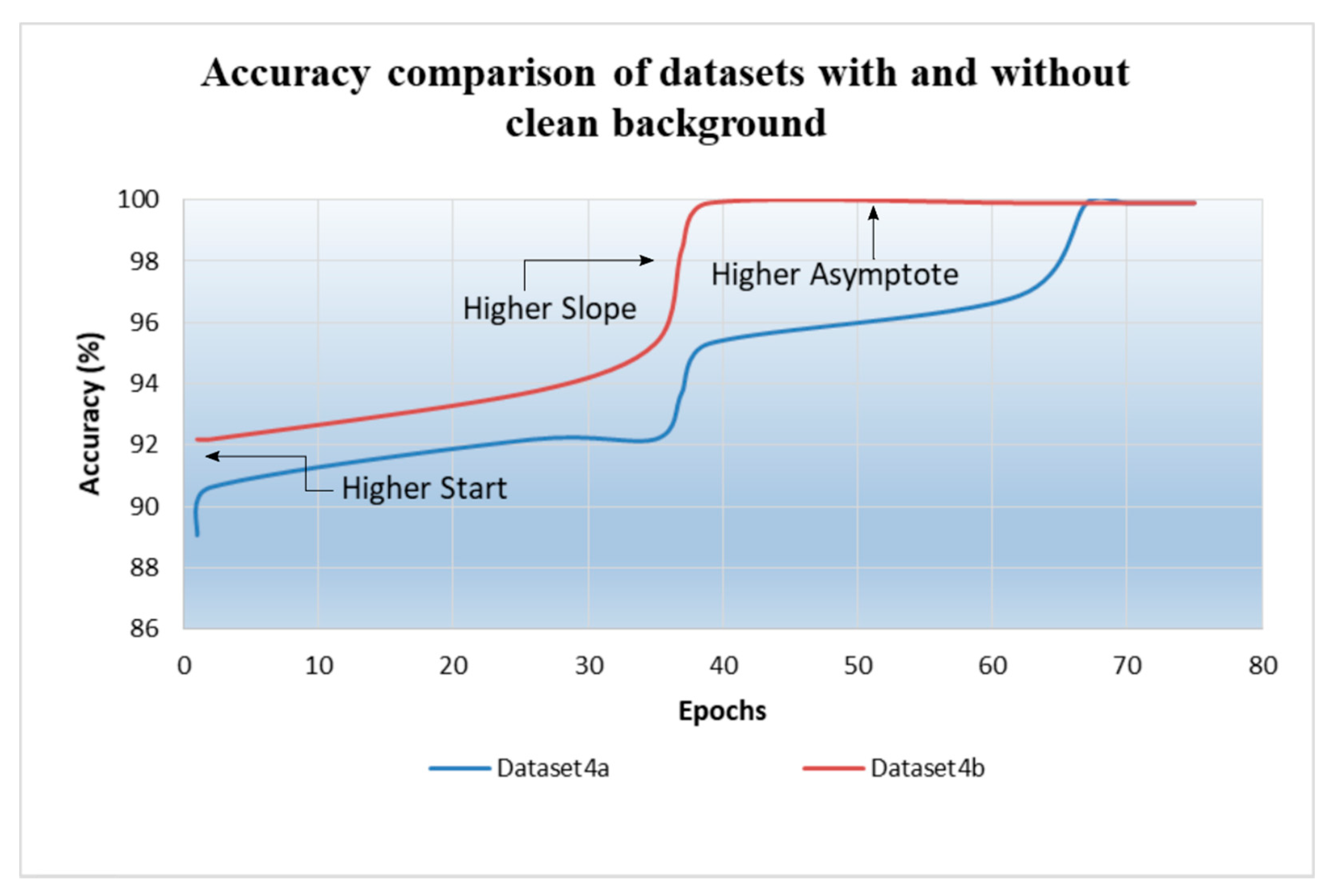
Figure 12 shows the training accuracy attained by fine-tuned MobileNet on dataset4a and dataset4b. It is evident that data with clean backgrounds train faster and have higher convergence compared to data with cluttered backgrounds.
4. Conclusions
In this work, different state-of-the-art fine-tuned deep models were employed and compared on image sets with different backgrounds. Segmentation and background subtraction algorithms were implemented to clean noisy background images. It is evident that the presence of a noisy background severely affects convolutional neural networks, which are seen through Grad-CAM visualization and reflected in their accuracy when trained and tested on data with high visual disparity. Segmentation algorithms isolated regions of interest from noisy backgrounds efficiently on images with higher depth between the subject of interest and background. Background subtraction algorithm improved background removal on images where the region of interest was interposed between the ill-favored foreground and background.
Fine-tuned models performed well on classifying plant diseases from leaf images. Removing background and training and testing models on clean data, significantly increased test accuracy. Fine-tuned DenseNet121 increased accuracy by 12% on a clean dataset compared to the dataset with cluttered images for the two-class dataset. Similarly, MobileNet and NA SNetMobile saw an increase in accuracy of 10 and 16%, respectively. The difference is highly pronounced when the number of classes in the dataset increase. The accuracy decreases when the number of classes increases. It dropped from 98.9% for two classes to 96.7% for four classes and finally to 93.57% for the eight-class dataset.
This study combined the concept of background removal using segmentation, background subtraction with convolutional neural network, and transfer learning to explore the impact of background noise on convolutional neural networks. The proposed image processing technique and deep learning approach showed higher efficacy on the plant leaf dataset, and its potential depends on the quality and quantity of available data. This study explored the potential of the noise removal algorithm and its effects on various network models.
Author Contributions
For Conceptualization, K.K. and Z.Y.; methodology, K.K.; software, K.K.; validation, K.K., Z.Y. and Z.W.; formal analysis, K.K.; investigation, K.K. and D.L.; resources, Z.Y.; data curation, D.L.; writing—original draft preparation, K.K.; writing—review and editing, K.K.; visualization, K.K.; supervision, Z.Y. and Z.W.; project administration, K.K.; funding acquisition, Z.Y. and Z.W. All authors have read and agreed to the published version of the manuscript.
Funding
The research presented in this article was supported by the National Natural Science Foundation of China (grant nos. 61471142, 61601145, 61571167, and 61871157).
Institutional Review Board Statement
Not applicable.
Informed Consent Statement
Not applicable.
Data Availability Statement
The data used in this study can be found at kamalchhetri24/Plant_disease_classification: Dataset for 8 classes of plant diseases (github.com) (accessed on 30 August 2021).
Conflicts of Interest
The authors declare no conflict of interest.
References
- Tajbakhsh, N.; Shin, J.Y.; Gurudu, S.R.; Hurst, R.T.; Kendall, C.B.; Gotway, M.B.; Liang, J. Convolutional Neural Networks for Medical Image Analysis: Full Training or Fine Tuning? IEEE Trans. Med. Imaging 2016, 35, 1299–1312. [Google Scholar] [CrossRef] [Green Version]
- Martinez-Gonzalez, A.N.; Villamizar, M.; Canevet, O.; Odobez, J.-M. Efficient Convolutional Neural Networks for Depth-Based Multi-Person Pose Estimation. IEEE Trans. Circ. Syst. Video Technol. 2020, 30, 4207–4221. [Google Scholar] [CrossRef] [Green Version]
- Simard, P.; Steinkraus, D.; Platt, J. Best practices for convolutional neural networks applied to visual document analysis. In Proceedings of the 7th International Conference on Document Analysis and Recognition, Edinburgh, UK, 3–6 August 2003; pp. 958–963. [Google Scholar]
- Li, Q.; Cai, W.; Wang, X.; Zhou, Y.; Feng, D.D.; Chen, M. Medical image classification with convolutional neural network. In Proceedings of the 2014 13th International Conference on Control Automation Robotics & Vision (ICARCV), Singapore, 10–12 December 2014; pp. 844–848. [Google Scholar]
- Kc, K.; Yin, Z.; Wu, M.; Wu, Z. Evaluation of deep learning-based approaches for COVID-19 classification based on chest X-ray images. Signal Image Video Process. 2021, 15, 959–966. [Google Scholar] [CrossRef]
- Zhao, K.; Kang, J.; Jung, J.; Sohn, G. Building extraction from satellite images using mask R-CNN with building bound-ary regularization. In Proceedings of the IEEE Conference on Computer Vision and Pattern Recognition Workshops, Salt Lake City, UT, USA, 18–22 June 2018; pp. 247–251. [Google Scholar]
- Amit, S.N.K.B.; Shiraishi, S.; Inoshita, T.; Aoki, Y. Analysis of satellite images for disaster detection. In Proceedings of the 2016 IEEE International Geoscience and Remote Sensing Symposium (IGARSS), Beijing, China, 10–15 July 2016; pp. 5189–5192. [Google Scholar]
- Yuan, Y.; Zheng, X.; Lu, X. Hyperspectral Image Superresolution by Transfer Learning. IEEE J. Sel. Top. Appl. Earth Obs. Remote Sens. 2017, 10, 1963–1974. [Google Scholar] [CrossRef]
- Mei, S.; Ji, J.; Hou, J.; Li, X.; Du, Q. Learning Sensor-Specific Spatial-Spectral Features of Hyperspectral Images via Convolutional Neural Networks. IEEE Trans. Geosci. Remote Sens. 2017, 55, 4520–4533. [Google Scholar] [CrossRef]
- Rajnoha, M.; Burget, R.; Povoda, L. Image Background Noise Impact on Convolutional Neural Network Training. In Proceedings of the 2018 10th International Congress on Ultra Modern Telecommunications and Control Systems and Workshops (ICUMT), Moscow, Russia, 5–9 November 2018; pp. 1–4. [Google Scholar]
- Singh, V.; Varsha Misra, A.K. Detection of unhealthy region of plant leaves using image processing and genetic algo-rithm. In Proceedings of the 2015 International Conference on Advances in Computer Engineering and Applications, Ghaziabad, India, 19–20 March 2015; pp. 1028–1032. [Google Scholar]
- Setitra, I.; Larabi, S. Background Subtraction Algorithms with Post-processing: A Review. In Proceedings of the 2014 22nd International Conference on Pattern Recognition, Stockholm, Sweden, 24–28 August 2014; pp. 2436–2441. [Google Scholar]
- Wang, K.; Gao, X.; Zhao, Y.; Li, X.; Dou, D.; Xu, C.-Z. Pay attention to features, transfer learn faster CNNs. In Proceedings of the International Conference on Learning Representations, New Orleans, LA, USA, 6–9 May 2019. [Google Scholar]
- Pan, S.J.; Yang, Q. A Survey on Transfer Learning. IEEE Trans. Knowl. Data Eng. 2010, 22, 1345–1359. [Google Scholar] [CrossRef]
- Yosinski, J.; Clune, J.; Bengio, Y.; Lipson, H. How Transferable Are Features in Deep Neural Networks? arXiv 2014, arXiv:1411.1792. [Google Scholar]
- Salman, H.; Ilyas, A.; Engstrom, L.; Kapoor, A.; Madry, A. Do adversarially robust imagenet models transfer better? arXiv 2020, arXiv:2007.08489. [Google Scholar]
- Mohanty, S.P.; Hughes, D.P.; Salathé, M. Using Deep Learning for Image-Based Plant Disease Detection. Front. Plant Sci. 2016, 7, 1419. [Google Scholar] [CrossRef] [PubMed] [Green Version]
- Arivazhagan, S.; Shebiah, R.N.; Ananthi, S.; Varthini, S.V. Detection of unhealthy region of plant leaves and classification of plant leaf diseases using texture features. Agric. Eng. Int. CIGR J. 2013, 15, 211–217. [Google Scholar]
- Singh, V.; Misra, A. Detection of plant leaf diseases using image segmentation and soft computing techniques. Inf. Process. Agric. 2017, 4, 41–49. [Google Scholar] [CrossRef] [Green Version]
- Al Bashish, D.; Braik, M.; Bani-Ahmad, S. Detection and classification of leaf diseases using K-means-based segmentation and. Inf. Technol. J. 2011, 10, 267–275. [Google Scholar] [CrossRef] [Green Version]
- Wang, Z.; Wang, K.; Yang, F.; Pan, S.; Han, Y. Image segmentation of overlapping leaves based on Chan–Vese model and Sobel operator. Inf. Process. Agric. 2018, 5, 1–10. [Google Scholar] [CrossRef]
- Chen, C.-T.; Su, C.-Y.; Kao, W.-C. An enhanced segmentation on vision-based shadow removal for vehicle detection. In Proceedings of the the 2010 International Conference on Green Circuits and Systems, Shanghai, China, 21–23 June 2010; pp. 679–682. [Google Scholar]
- Jamal, I.; Akram, M.U.; Tariq, A. Retinal Image Preprocessing: Background and Noise Segmentation. TELKOMNIKA (Telecommun. Comput. Electron. Control. 2012, 10, 537–544. [Google Scholar] [CrossRef]
- Kussul, N.; Lavreniuk, M.; Skakun, S.; Shelestov, A. Deep Learning Classification of Land Cover and Crop Types Using Remote Sensing Data. IEEE Geosci. Remote Sens. Lett. 2017, 14, 778–782. [Google Scholar] [CrossRef]
- Kc, K.; Yin, Z.; Wu, M.; Wu, Z. Depthwise separable convolution architectures for plant disease classification. Comput. Electron. Agric. 2019, 165, 104948. [Google Scholar] [CrossRef]
- Deng, J.; Dong, W.; Socher, R.; Li, L.J.; Li, K.; Li, F.F. Imagenet: A Large-Scale Hierarchical Image Database. In Proceedings of the 2009 IEEE Conference on Computer Vision and Pattern Recognition, Miami, FL, USA, 20–25 June 2009; pp. 248–255. [Google Scholar]
- Kamal, K.; Yin, Z.; Li, B.; Ma, B.; Wu, M. Transfer Learning for Fine-Grained Crop Disease Classification Based on Leaf Images. In Proceedings of the 2019 10th Workshop on Hyperspectral Imaging and Signal Processing: Evolution in Remote Sensing (WHISPERS), Amsterdam, The Netherlands, 24–26 September 2019. [Google Scholar]
- Chen, J.; Chen, J.; Zhang, D.; Sun, Y.; Nanehkaran, Y. Using deep transfer learning for image-based plant disease identification. Comput. Electron. Agric. 2020, 173, 105393. [Google Scholar] [CrossRef]
- Barbedo, J.G.A. Impact of dataset size and variety on the effectiveness of deep learning and transfer learning for plant disease classification. Comput. Electron. Agric. 2018, 153, 46–53. [Google Scholar] [CrossRef]
- Nayak, A.A.; Venugopala, P.S.; Sarojadevi, H.; Chiplunkar, N.N. An approach to improvise canny edge detection using morphological filters. Int. J. Comput. Appl. 2015, 116, 38–42. [Google Scholar]
- Mandellos, N.A.; Keramitsoglou, I.; Kiranoudis, C.T. A background subtraction algorithm for detecting and tracking vehicles. Expert Syst. Appl. 2011, 38, 1619–1631. [Google Scholar] [CrossRef]
- Simonyan, K.; Zisserman, A. Very Deep Convolutional Networks for Large-Scale Image Recognition. arXiv 2014, arXiv:1409.1556. [Google Scholar]
- Kaiming, H.; Xiangyu, Z.; Shaoqing, R.; Jian, S. Deep Learning with Depthwise Separable Convolutions. In Proceedings of the IEEE Conference on Computer Vision and Pattern Recognition (CVPR), Honolulu, HI, USA, 21–26 July 2017; pp. 1251–1258. [Google Scholar]
- Szegedy, C.; Liu, W.; Jia, Y.; Sermanet, P.; Reed, S.; Anguelov, D.; Erhan, D.; Vanhoucke, V.; Rabinovich, A. Going deeper with convolutions. In Proceedings of the IEEE Conference on Computer Vision and Pattern Recognition, Boston, MA, USA, 7–12 June 2015; pp. 1–9. [Google Scholar] [CrossRef] [Green Version]
- Howard, A.G.; Zhu, M.; Chen, B.; Kalenichenko, D.; Wang, W.; Weyand, T.; Andreetto, M.; Adam, H. Mobilenets: Efficient convolutional neural networks for mobile vision applications. arXiv 2017, arXiv:1704.04861. [Google Scholar]
- Sandler, M.; Howard, A.; Zhu, M.; Zhmoginov, A.; Chen, L.-C. MobileNetV2: Inverted Residuals and Linear Bottlenecks. In Proceedings of the 2018 IEEE/CVF Conference on Computer Vision and Pattern Recognition, Salt Lake City, UT, USA, 18–23 June 2018; pp. 4510–4520. [Google Scholar]
- Huang, G.; Liu, Z.; Van Der Maaten, L.; Weinberger, K.Q. Densely Connected Convolutional Networks. In Proceedings of the 2017 IEEE Con-ference on Computer Vision and Pattern Recognition (CVPR), Honolulu, HI, USA, 21–26 July 2017; pp. 2261–2269. [Google Scholar]
- Zoph, B.; Vasudevan, V.; Shlens, J.; Le, Q.V. Learning Transferable Architectures for Scalable Image Recognition. In Proceedings of the 2018 IEEE/CVF Conference on Computer Vision and Pattern Recognition, Salt Lake City, UT, USA, 18–23 June 2018; p. 18311827. [Google Scholar]
- Hughes, D.P.; Salathé, M. An open access repository of images on plant health to enable the development of mobile disease diagnostics through machine learning and crowdsourcing. arXiv 2015, arXiv:1511.08060. [Google Scholar]
- Selvaraju, R.R.; Cogswell, M.; Das, A.; Vedantam, R.; Parikh, D.; Batra, D. Grad-CAM: Visual Explanations from Deep Networks via Gradient-Based Localization. In Proceedings of the 2017 IEEE International Conference on Computer Vision (ICCV), Venice, Italy, 22–29 October 2017; pp. 618–626. [Google Scholar] [CrossRef] [Green Version]
- Ferentinos, K.P. Deep learning models for plant disease detection and diagnosis. Comput. Electron. Agric. 2018, 145, 311–318. [Google Scholar] [CrossRef]
- Wang, G.; Sun, Y.; Wang, J. Automatic Image-Based Plant Disease Severity Estimation Using Deep Learning. Comput. Intell. Neurosci. 2017, 2017, 1–8. [Google Scholar] [CrossRef] [PubMed] [Green Version]
Figure 1.
A single biological neuron is annotated to describe a single artificial neural function.

Figure 2.
Images with an undesired background. (a) Leaf image in situ, the top image contains a leaf from another species on top of the region of interest; the bottom two contain mud on top of the healthy leaf, appearing to be diseased; (b) image with the human hand in the foreground; (c) segmentation result of the image on the left.

Figure 3.
A framework of the proposed method.
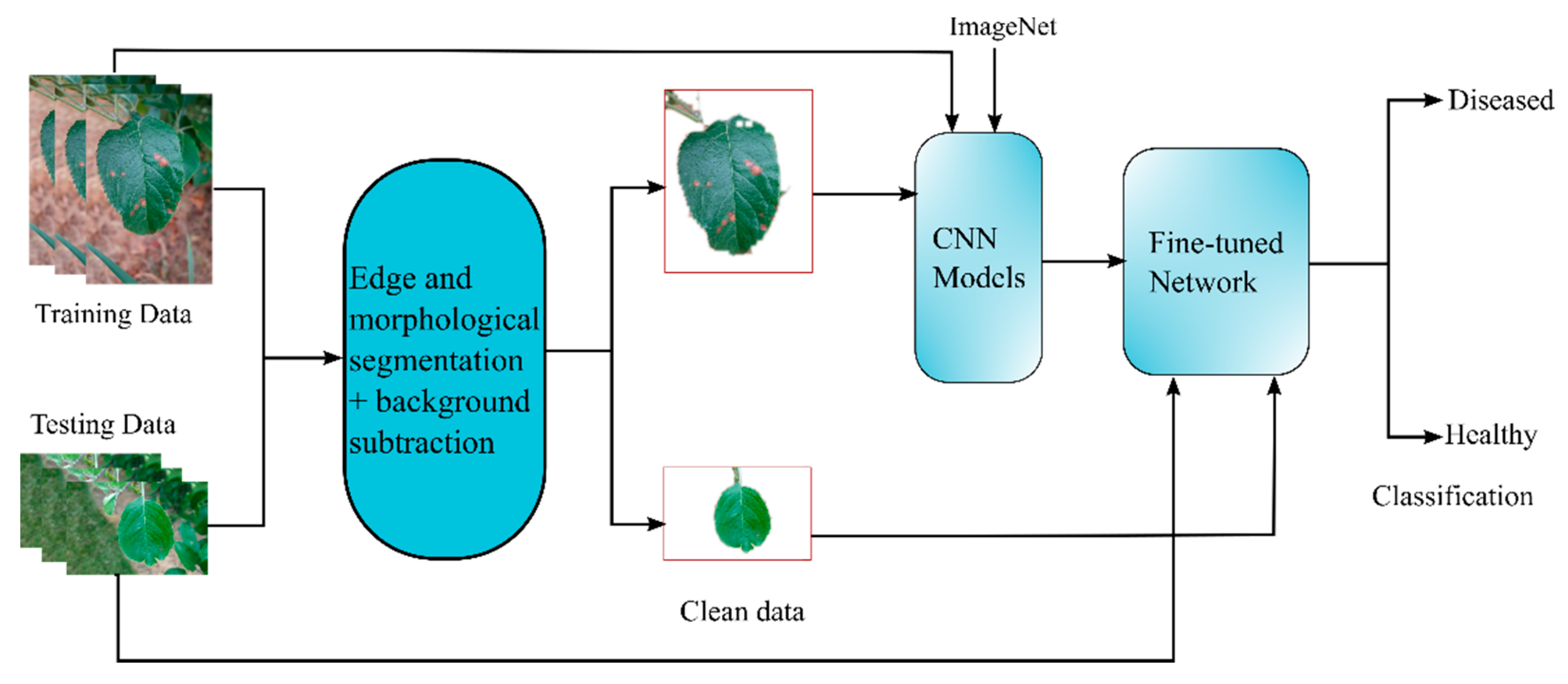
Figure 4.
Removing foreground objects using background subtraction.

Figure 5.
VGG19 was retrained as a feature extractor and fine-tuned for better accuracy by retraining convolutional blocks.
Figure 5.
VGG19 was retrained as a feature extractor and fine-tuned for better accuracy by retraining convolutional blocks.

Figure 6.
Information of the plant leaf dataset. The complete dataset is divided into four categories with two, four, and eight classes.
Figure 6.
Information of the plant leaf dataset. The complete dataset is divided into four categories with two, four, and eight classes.

Figure 7.
Results of background removal algorithm. (a) Input images; (b) canny edge detection; (c) edge dilation; (d) edge erosion; (e) mask dilation; (f) mask erosion; (g) Gaussian blur; (h) background removed image.
Figure 7.
Results of background removal algorithm. (a) Input images; (b) canny edge detection; (c) edge dilation; (d) edge erosion; (e) mask dilation; (f) mask erosion; (g) Gaussian blur; (h) background removed image.

Figure 8.
Segmented image and corresponding clean background output image.

Figure 9.
Visualization using Grad-CAM for plant leaf image.
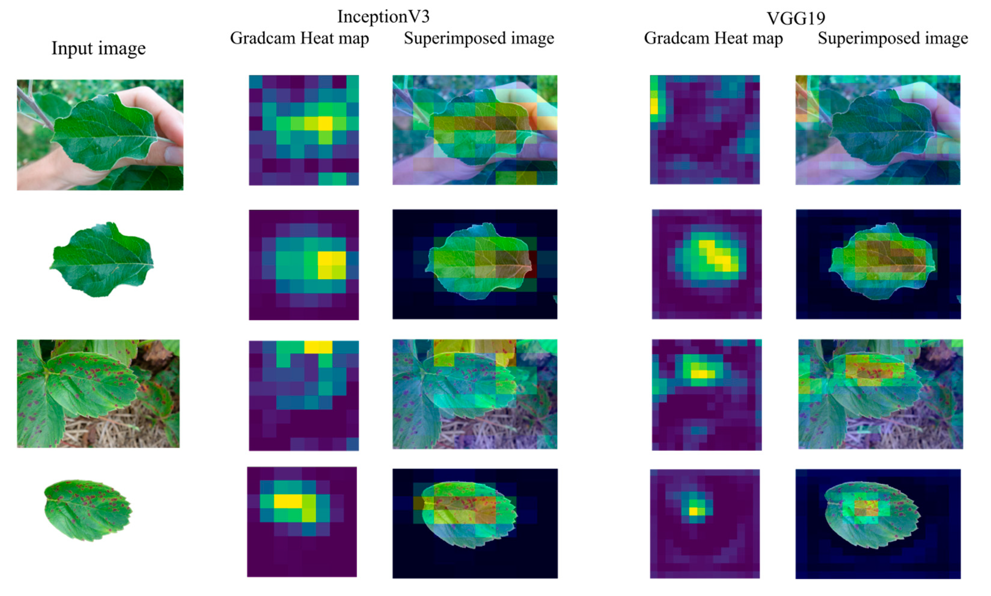
Figure 10.
Testing accuracy achieved by various pre-trained fine-tuned CNN models on a different number of classes of datasets. Dataset1a, dataset2a, and dataset3a contain testing images taken in true field conditions. Dataset1b, dataset2b, and dataset3b contain the test images cleaned with the proposed background removal algorithm.

Figure 11.
Confusion matrices for two, four, and eight class datasets. Confusion matrices obtained from fine-tuned (a) DenseNet121, (b) InceptionV3, and (c) DenseNet121 models for datase1b, dataset2b, and dataset3b, respectively.
Figure 11.
Confusion matrices for two, four, and eight class datasets. Confusion matrices obtained from fine-tuned (a) DenseNet121, (b) InceptionV3, and (c) DenseNet121 models for datase1b, dataset2b, and dataset3b, respectively.

Figure 12.
Comparing the accuracy of fine-tuned MobileNet on image sets (cabbage leaves) with and without clean background.
Figure 12.
Comparing the accuracy of fine-tuned MobileNet on image sets (cabbage leaves) with and without clean background.


Table 1.
CNN Training hyperparameters and data augmentation techniques.
| Hyperparameters | Data Augmentation | |
|---|---|---|
| Optimizer | Nadam | Rescaling |
| Learning rate | Horizontal flip | |
| Exponential decay rate () | 0.9 | Zoom range = 0.3 |
| Exponential decay rate () | 0.999 | Width shift range = 0.3 |
| Epsilon (ε) | Height shift range = 0.3 | |
| Batch size | 128 | Rotation range = 30 |
| Maximum epoch | 500 | Zca whitening |
| Activation function | Rectified Linear Unit (ReLU) | Zca epsilon = |
Table 2.
Classification performance indicators of various fine-tuned models on dataset2.
| Dataset1b | Dataset2b | Dataset3b | ||
|---|---|---|---|---|
| Metrics | DenseNet121 | InceptionV3 | DenseNet121 | |
| Models | ||||
| Precision | 0.9944 | 0.9829 | 0.9639 | |
| Recall | 0.9888 | 0.9773 | 0.9524 | |
| Specificity | 0.9878 | 0.963 | 0.9240 | |
| F1-score | 0.9916 | 0.98 | 0.958 | |
| Accuracy (%) | 98.9 | 96.7 | 93.57 | |
Table 3.
A comparison of different CNN networks employed to classify plant disease with the proposed network.
Table 3.
A comparison of different CNN networks employed to classify plant disease with the proposed network.
| Related Work | Accuracy (%) | Classes | Total Images | Train-Test Split (%) | Model |
|---|---|---|---|---|---|
| Mohanty et al. [17] | 31.4 | - | 121 | 80–20 | GoogLeNet |
| Ferentinos et al. [41] | 33.27 | 12 | - | 55.8–44.2 | VGG |
| Kamal et al. [25] | 36.03 | 11 | 22110 | 48.1–51.9 | MobileNet |
| Wang et al. [42] | 90.4 | 4 | 2086 | 80–20 | Fine-tuned InceptionV3 |
| Proposed system (Cluttered background) | 87.12 | 2 | 1262 | 80–20 | Fine-tuned Densenet121 |
| Proposed system (Background removed) | 93.57 | 8 | 4558 | 80–20 | Fine-tuned Densenet121 |
Publisher’s Note: MDPI stays neutral with regard to jurisdictional claims in published maps and institutional affiliations. |
© 2021 by the authors. Licensee MDPI, Basel, Switzerland. This article is an open access article distributed under the terms and conditions of the Creative Commons Attribution (CC BY) license (https://creativecommons.org/licenses/by/4.0/).
Share and Cite
MDPI and ACS Style
KC, K.; Yin, Z.; Li, D.; Wu, Z. Impacts of Background Removal on Convolutional Neural Networks for Plant Disease Classification In-Situ. Agriculture 2021, 11, 827. https://0-doi-org.brum.beds.ac.uk/10.3390/agriculture11090827
AMA Style
KC K, Yin Z, Li D, Wu Z. Impacts of Background Removal on Convolutional Neural Networks for Plant Disease Classification In-Situ. Agriculture. 2021; 11(9):827. https://0-doi-org.brum.beds.ac.uk/10.3390/agriculture11090827
Chicago/Turabian StyleKC, Kamal, Zhendong Yin, Dasen Li, and Zhilu Wu. 2021. "Impacts of Background Removal on Convolutional Neural Networks for Plant Disease Classification In-Situ" Agriculture 11, no. 9: 827. https://0-doi-org.brum.beds.ac.uk/10.3390/agriculture11090827
Note that from the first issue of 2016, this journal uses article numbers instead of page numbers. See further details here.