Analysis of Heat and Mass Distribution in a Single- and Multi-Span Greenhouse Microclimate

Abstract

Recently, heat and mass distributions within a greenhouse were assumed to be homogeneous. Heat is gained or lost in absolute terms, and crop contribution in a greenhouse or its effect is not considered. In this study, statistical analyses were conducted to establish the significance of heat and mass variation at sensor nodes in two single-span and multi-span greenhouses. Three greenhouses were used in this study, 168 m² floor area a single-layered (SLG), double-layered (DLG) single-span gothic roof type greenhouses, and 7572.6 m² floor area multi-span greenhouse (MSG). The microclimatic parameters investigated were temperature (T), relative humidity (RH), solar radiation (SR), carbon dioxide (CO₂), and vapor pressure deficit (VPD). To check their horizontal distribution, all microclimate data collected from each sensor node in each greenhouse were subjected to descriptive statistics and Tukey honestly significant difference (HSD) test. The lowest minimum temperatures of 2.93 °C, 3.33 °C and 10.50 °C were recorded at sensor points in SLG, DLG, and MSG, respectively, whereas the highest maximum temperatures of 29.17 °C, 29.07 °C and 27.20 °C were recorded at sensor point, in SLG, DLG, and MSG, respectively. The difference between the center and the side into the single-span was approximately 0.88–1.0 °C and in the MSG was approximately 1.03 °C. Significant variation was observed in the horizontal distribution of T, RH, SR, and VPD within SLG, DLG, and MSG. Also significant was CO₂ in the MSG. Estimating the energy demand of greenhouses should be done based on the distribution rather than assuming microclimatic parameters homogeneity, especially for T, with VPD as a control parameter. Such estimation should also be done using a crop model that considers instant changes in air and crop temperature.

1. Introduction

A greenhouse is an agricultural structure used in protecting crops from harmful and extreme weather conditions. Energy is required to heat up or cool down greenhouse microclimate in the winter and summer, respectively. Therefore, the energy demand of the greenhouse should be estimated. The estimation can be done theoretically or using energy simulation models such as TRNSYS [1,2,3], energy plus, and so on. The tools accept energy-related microclimate parameters and return the estimated energy as output. Microclimate parameters are distributed homogeneously or heterogeneously within a greenhouse and are determined by the heat and mass distributions within the greenhouse. Temperature, radiation, and dew point temperature are heat-related parameters, whereas relative humidity (RH) (moisture), CO₂, and vapor pressure deficit (VPD) are mass-related. Optimal crop growth in a greenhouse requires optimal temperature, humidity, carbon dioxide, and solar radiation [4,5,6,7]. Mass and heat transfer phenomena (e.g., evaporation, condensation, photosynthesis, and climate change) affect the quality and quantity of the produced crops.

Previous studies focused on the vertical component of the environmental parameters within greenhouses, and most of these studies have discovered significant temperature gradients, even though the experiments were conducted in small greenhouses [8,9] found a 4.5–5 °C temperature difference between the top and bottom of the greenhouse canopy. According to [10], the highest temperatures were found nearer the roof, with a difference of 5 °C between the coolest and warmest points. However, temperature gradients were increased by 14% in the presence of crops. Nevertheless, ref. [11] has already reported a temperature difference of 6 °C near the roof, just above the crop canopy. Ref. [12] studied the distribution of temperature, humidity, and photosynthetic photon flux (PPF) in a double-covering-conventional and air-inflated greenhouse used for tomato production and reported a temperature difference of 3.5 °C between a double-layered-conventional and air-inflated greenhouse and a lower PPF in a conventional greenhouse. Recently, ref. [13] compared the averaged microclimate parameters of polyolefin–thermal screen (PoTS) and polyolefin–thermal screen–polyethylene (PoTSPe) glazed greenhouse used for strawberry cultivation and reported that more energy was consumed in the PoTS than in PoTSPe. Ref. [14] used wireless sensor networks in mechanically and naturally ventilated and shaded greenhouses to describe and chart the horizontal and vertical variability in air temperature and RH within a greenhouse, concluding that there was a horizontal homogeneity among the sensors.

Most studies have reported using more than one sensor [1,2,3,15], but mainly use mean sensor values to estimate the energy demand of greenhouse. Some researchers [16,17] also assumed that greenhouse aerial temperature is the same in all directions. However, using the mean is not a good representation of a group of scores [18]. Furthermore, only a single sensor is used to set the greenhouse microclimate control. In this regard, if there is a significant difference among sensor values, there may be over or underestimation of energy demand, and some crops might be exposed to unfavorable climatic conditions [19]. Additionally, mean values are not always predicted correctly [20]. Therefore, further studies should investigate the distribution of environmental variables within the greenhouse, evaluating the presence of hot spots.

Previously, some researchers assumed that crop evapotranspiration in greenhouse energy estimation was positive, while other researchers considered that it was negative [3,15] examined the results of a plant-air interaction using a 90% cultivated fraction of the greenhouse floor and a mass surface density of 10 kg/m². They concluded that the heat loss during the daytime is the highest during the summer months, because of the higher transpiration rates and longer sunlight hours per day, whereas the opposite occurs during the nighttime. Considering this context, this study analyzes horizontal heat and mass distribution within a greenhouse microclimate and the interaction of the crop-air temperature.

2. Materials and Methods

2.1. Profile of the Experimental Greenhouse

2.1.1. Single-Span Greenhouses

A double-layer (DLG) and single-layer (SLG) greenhouse were built in Daegu, South Korea, located at 35.53° N, 128.36° E, and 48 m above sea level. As shown in Figure 1, both greenhouses are single-span, gothic-type roofs covered with polyolefin (PO) and polyethylene (PE), and only PO material, respectively, a single-layer thermal screen, and E-W orientation. With a gross volume of 553.1 m³ and a floor area of 168 m², the dimensions were 24 × 7 × 4 m. Natural side and roof ventilation were used in both greenhouses. Ref. [21] had studied the efficiency of natural ventilation on these greenhouses (Figure A1 is as presented in the Appendix A). During the day, both greenhouses are single-layer, but at night, the polyethylene that makes up the second layer in the DLG is deployed (hence, double layer). The roof vent of the DLG is open on both sides, whereas the roof vent of SLG is opened only on one side (Figure 1). The SLG floor is covered with a layer of granite, whereas the DLG is covered with tarpaulin, the effects of which were studied as greenhouse features rather than the heat and mass distribution. In each greenhouse, six fans of 25 m³/min flow rate were installed, three at each end facing the opposite direction to enable a better mixture of mass and heat within the greenhouse. The sensors and fans are shown in Figure 2. The greenhouses were temperature-controlled, with minimum and maximum interior temperatures between 8 °C and 23 °C, respectively. The roof and side vents open when the temperature exceeds 21 °C and 23 °C and close when the temperature falls below the minimum temperature setpoints. The heat source was a diesel-fired boiler connected to heating pipes that run through the greenhouse. When the temperature inside the greenhouse falls below 8 °C, the boiler turned on and the hot water was pumped through the heating pipes, to raise the microclimate temperature until the temperature reached the minimum setpoint of 8 °C, at which it turned off until the temperature fell below again. The sensor at position C2 controls the opening and closing of the roof and side vents, as well as the powering of the boiler. The thermal screens in both greenhouses were scheduled to close and open at 6.00 pm and 8.30 am, respectively, whereas the PE screen in DLG was scheduled to open and close by 9.00 am and 5.30 pm, respectively. Strawberry (Seolhyang sp.) was cultivated during the experimental period in both greenhouses.

2.1.2. Multi-Span Greenhouse (MSG)

The multi-span greenhouse (MSG) was built in an N–S orientation in Taean Gun, Chungcheongnam-do, South Korea, located at 36.88° N, 126.24° E, and 45 m above sea level. The greenhouse has a Venlo-style roof with 15 spans. The dimension, floor area, and span width of the greenhouse were 63 × 120.2 × 7.48 m, 7572.6 m², and 8 m, respectively. The sides and roof were made of polycarbonate (PC) and horticulture glass (HG), which were 16 and 4 mm thick, respectively. In the greenhouse, thirty 100 m³/min flow rate fans were installed in alternate directions, as shown in Figure 3b. The aim is to create a better mixture of mass and heat within the greenhouse. One PH_77 thermal screen with thermal conductivity and thickness of 0.59 W/mK and 0.4 mm, respectively, and two PH-Super thermal screens with thermal conductivity and thickness 0.08 W/mK and 0.3 mm, respectively, were installed directly under the HG roof, with a layer of the PH_77 thermal screen installed on the greenhouse sidewalls. The vertical and horizontal views of the full specifications are shown in Figure 3a,b, respectively. Strawberries (Seolhyang sp.) were also cultivated in the MSG during the experimental period.

The greenhouse temperature was controlled within a range of 15 °C and 19 °C as the minimum and maximum temperatures, respectively. The roof vent opened and closed when the temperatures were above 19 °C and below 15 °C, respectively, while the thermal screens are scheduled as follows:

Thermal screen 1: opened after sunrise or temperature is 10 °C or SR is 100 W.

Closed after sunset or temperature are 12 °C and SR is 100 W.

Thermal screen 2: opened after sunrise or temperature is 5 °C or SR is 50 W.

Closed after sunset or temperature are 12 °C and SR is 50 W.

Thermal screen 3: opened after sunrise or temperature is 12 °C or SR is 150 W.

Closed after sunset or temperature are 14 °C and SR is 150 W.

2.2. Data Collection

2.2.1. Single-Span Greenhouse

Nine Hobo onset U23-002 sensors with a sensitivity of ±0.21 °C (from 0–50 °C) and ±2.5% (from 10–100% RH) were installed horizontally immediately above the strawberry plants to record the air temperature (T), dew point temperature (T_dp), and relative humidity (RH). Furthermore, two Kipp and Zonen pyranometers (CMP3 model) with a sensitivity of <5%, −10–40 °C, and spectral range of 300–2800 nm were installed to record the solar radiation (SR) received at those points. The distance and positions of the sensors are shown in Figure 2. The condition of the crops in the greenhouse is affected by the microclimate condition. Therefore, the temperatures and RH sensors were chosen to measure the condition near most of the crops, as well as the sides and center of the greenhouse. All sensors recorded data every 10 min. The data were collected from 1 November 2020, to 3 March 2021. After data extraction and processing, the VPD at the respective sensor points was calculated using Equations (1) and (2). An Apogee infrared radiometer surface temperature sensor of model SI-131-SS with an uncertainty of ±0.3 °C (ranging from −30–65 °C) was installed to measure the leaf surface temperature (Figure 2).

2.2.2. Multi-Span Greenhouse

To record the air temperature (T) and RH, four SHT75 Sensirion sensors with a sensitivity of 0–100% RH ± 1.8% and −40–123.8 °C ± 0.3 °C were horizontally installed at the immediate site of the strawberry plants. Unlike SLG and DLG, MSG has four installed sensors because stratification occurs more easily in large spaces, also, due to a limited number of sensors. Four Kipp and Zonen pyranometers (CMP3 model) with a sensitivity <5%, −10 °C–40 °C and spectral range of 300–2800 nm were also installed to record the solar radiation and four TR-76UI-H Tecpel CO₂ sensors with a sensitivity of ±50 ppm were installed to measure CO₂ at those points. The distance and positions of the sensors are shown in Figure 3. The data was collected from 25 December 2020, to 7 January 2021, and the data logging interval for all sensors was 1 min.

After data extraction and processing, the VPD at the respective sensor points were calculated using Equations (1) and (2).

$$SVP=610.78\times {2.71828}^{\left(\frac{T}{T+273}\times 17.2694\right)}$$

(1)

$$VPD=SVP\times (1-\frac{RH}{100})$$

(2)

2.3. Data Analysis

All data collected for each sensor in each greenhouse were subjected to descriptive statistics and analysis of variance (ANOVA) using the Microsoft Excel 2019 statistical package. The level of significant variations among the sensors in the single-span and multi-span greenhouses was conducted using horizontal distribution analysis. The sensors that were significantly different from each other were subjected to Tukey honestly significant difference (HSD) test.

The interaction between the greenhouse crops and the air temperature was also analyzed.

3. Results and Discussion

3.1. Single-Span Greenhouse

3.1.1. Heat and Mass Variation

The descriptive statistics of the distribution of microclimate parameters for all sensors are presented in

Table 1. Descriptive statistics of T, RH, T_dp, and VPD distributions in SLG. SD: standard deviation; Min.: minimum; Max.: maximum; RH: relative humidity; T_dp: dew point temperature; VPD: vapor pressure deficit; SLG: single-layered greenhouse.

Parameter	Description	A1	A2	A3	C1	C2	C3	E1	E2	E3
T (°C)	Mean	12.79	12.80	12.53	12.83	13.35	12.83	12.70	12.60	12.11
	Median	11.05	11.05	10.93	11.25	11.42	11.13	11.18	11.27	10.91
	Mode	7.52	7.52	7.47	7.72	8.82	7.62	7.67	7.72	7.42
	SD	4.99	5.05	4.81	4.76	5.28	4.85	4.71	4.29	4.12
	Min.	2.93	3.30	2.85	3.17	4.12	3.33	2.90	3.56	2.96
	Max.	29.17	29.09	29.04	29.17	29.14	28.97	27.75	26.11	26.21
	Sum	225,775.99	226,074.66	221,288.56	226,502.90	235,782.19	226,614.26	224,185.28	222,483.19	213,773.05
RH (%)	Mean	72.57	76.72	76.97	75.55	75.99	75.90	76.36	77.51	77.97
	Median	81.60	85.57	84.59	83.00	84.69	84.02	85.06	84.26	85.16
	Mode	84.57	91.03	90.63	90.64	91.51	90.54	90.76	91.32	90.81
	SD	17.76	19.92	18.57	18.40	20.00	19.22	19.94	17.02	18.01
	Min.	13.00	17.10	18.99	18.82	18.58	18.04	16.45	20.89	17.98
	Max.	85.79	97.75	97.58	96.77	98.38	97.19	97.98	97.26	97.89
	Sum	1,281,503.08	1,354,745.47	1,359,120.15	1,334,000.14	1,341,787.75	1,340,154.40	1,348,420.61	1,368,657.82	1,376,706.16
Tdp (°C)	Mean	7.28	8.01	7.91	7.94	8.38	7.94	7.85	8.23	7.76
	Median	6.68	7.33	7.19	7.22	7.66	7.24	7.23	7.53	7.20
	Mode	4.92	6.41	5.99	6.14	11.41	6.20	6.53	6.31	6.15
	SD	3.31	3.56	3.56	3.48	3.44	3.59	3.65	3.50	3.72
	Min.	−7.89	−4.79	−4.77	−4.94	−3.32	−5.54	−6.71	−4.94	−7.27
	Max.	20.63	21.77	22.61	22.11	22.19	22.54	21.84	22.88	22.00
	Sum	128,635.57	141,357.52	139,635.59	140,202.36	147,988.51	140,290.91	138,591.04	145,344.18	137,075.71
VPD (kPa)	Mean	0.50	0.45	0.42	0.45	0.49	0.45	0.44	0.39	0.37
	Median	0.25	0.19	0.20	0.22	0.20	0.21	0.19	0.21	0.19
	Mode	0.17	0.10	0.15	0.15	0.15	0.15	0.16	0.14	0.15
	SD	0.53	0.53	0.48	0.48	0.57	0.50	0.49	0.39	0.39
	Min.	0.12	0.07	0.07	0.08	0.06	0.07	0.06	0.07	0.06
	Max.	3.06	2.95	3.00	2.91	2.96	2.97	2.76	2.48	2.52
	Sum	8910.40	7979.37	7502.32	7968.27	8620.88	7993.55	7782.34	6950.87	6595.67
	Count	17,658.00	17,658.00	17,658.00	17,658.00	17,658.00	17,658.00	17,658.00	17,658.00	17,658.00

,

Table 2. Descriptive statistics of T, RH, T_dp, and VPD distributions in DLG. SD: standard deviation; Min.: minimum; Max.: maximum. T: air temperature; RH: relative humidity; T_dp: dew point temperature; VPD: vapor pressure deficit; DLG: double-layered greenhouse.

Parameter	Description	A1	A2	A3	C1	C2	C3	E1	E2	E3
T (°C)	Mean	13.21	12.91	12.47	13.20	13.34	12.64	12.96	12.53	12.34
	Median	11.42	11.27	11.01	11.49	11.64	11.22	11.35	11.22	11.08
	Mode	8.82	7.87	8.02	8.87	8.52	8.42	7.87	9.31	8.67
	SD	5.28	5.05	4.81	5.19	5.14	4.67	4.99	4.45	4.44
	Min.	3.56	3.56	3.33	3.64	3.91	3.70	3.64	3.62	3.51
	Max.	28.49	27.36	27.92	29.07	28.99	28.42	27.73	26.21	26.92
	Sum	233,245.80	228,029.07	220,183.48	233,157.38	235,517.34	223,116.99	228,883.83	221,263.42	217,878.43
RH (%)	Mean	79.07	80.35	81.62	79.04	79.86	80.92	80.05	81.57	82.02
	Median	91.97	92.09	93.44	91.05	92.22	91.81	91.76	91.96	92.41
	Mode	95.29	96.13	95.55	94.36	93.77	95.20	95.97	95.35	95.24
	SD	23.41	21.77	22.20	22.35	22.40	20.96	21.78	20.12	19.98
	Min.	12.73	16.27	14.76	15.14	15.49	16.58	17.51	18.75	18.60
	Max.	98.31	98.87	99.50	98.58	99.18	98.64	99.49	99.47	98.84
	Sum	1,396,171.66	1,418,874.66	1,441,173.76	1,395,665.30	1,410,111.87	1,428,888.90	1,413,535.44	1,440,319.46	1,448,323.00
Tdp (°C)	Mean	8.46	8.63	8.38	8.59	8.88	8.54	8.64	8.66	8.56
	Median	8.09	8.18	8.05	8.14	8.46	8.11	8.15	8.16	8.12
	Mode	6.43	7.13	5.90	7.83	6.33	6.61	6.28	7.15	7.35
	SD	3.76	3.65	3.79	3.61	3.53	3.61	3.63	3.59	3.60
	Min.	−7.86	−6.45	−9.04	−5.71	−5.18	−7.01	−5.80	−5.28	−6.31
	Max.	21.56	22.01	21.12	21.80	21.72	21.00	22.56	22.36	21.36
	Sum	149,390.75	152,473.18	148,027.80	151,618.70	156,770.67	150,863.41	152,522.42	152,942.62	151,168.81
VPD (kPa)	Mean	0.46	0.41	0.38	0.45	0.44	0.38	0.42	0.36	0.35
	Median	0.12	0.12	0.10	0.13	0.12	0.12	0.12	0.12	0.12
	Mode	0.07	0.08	0.06	0.12	0.08	0.08	0.07	0.06	0.07
	SD	0.63	0.54	0.53	0.59	0.59	0.50	0.53	0.44	0.44
	Min.	0.06	0.05	0.05	0.06	0.05	0.05	0.05	0.05	0.05
	Max.	2.95	2.68	2.81	3.02	2.91	2.85	2.65	2.53	2.56
	Sum	8181.67	7300.08	6709.50	7985.00	7819.08	6757.94	7355.64	6302.59	6107.11
	Count	17,658.00	17,658.00	17,658.00	17,658.00	17,658.00	17,658.00	17,658.00	17,658.00	17,658.00

,

Table 3. Descriptive statistics of SR in SLG (single-layered greenhouse). SR: solar radiation; C2 and E2: control and experimental sensors; SD: standard deviation; Min.: minimum; Max.: maximum.

	SR (W/m2)
	C2	E2
Mean	200.29	103.07
Median	163.99	85.79
Mode	10.93	77.12
SD	157.97	75.23
Min.	7.29	8.67
Max.	647.23	532.93
Sum	1,347,972.30	693,658.58
Count	6730.00	6730.00

and

Table 4. Descriptive statistics of the SR in DLG (double-layered greenhouse). SR: solar radiation; C2 and E2: control and experimental sensors; SD: standard deviation; Min.: minimum; Max.: maximum.

	SR (W/m2)
	C2	E2
Mean	215.65	112.66
Median	181.41	103.56
Mode	9.68	25.24
SD	167.11	76.64
Min.	9.04	8.41
Max.	653.97	717.15
Sum	1,420,052.29	741,862.14
Count	6585.00	6585.00

. The control sensor minimum and maximum values for SLG (Table 1 and Table 3) were 4.12 °C and 29.14 °C, 18.95%, and 98.38%, 3.32 °C and 22.19 °C, 0.06 kPa, and 2.96 kPa, and 7.29 W/m² and 647.23 W/m², for T, RH, Tdp, VPD, and SR, respectively. The control sensor minimum and maximum values for DLG (Table 2 and Table 4) were 3.91 °C and 28.99 °C, 15.49%, and 99.18%, 5.18 °C, and 21.72 °C, 0.05 kPa, and 2.91 kPa, and 9.04 W/m² and 653.97 W/m². The percentage change in the parameter sum between control (C2) and other sensors in SLG and DLG are shown in

Table 5. Percentage change in parameter sum between the control sensor and the other sensors in SLG (single-layered greenhouse) T: air temperature; RH: relative humidity; T_dp: dew point temperature; VPD: vapor pressure deficit; SR: solar radiation.

Parameter	Position	A1	A2	A3	C1	C3	E1	E2	E3
T	Control sensor (C2)	+4.43	+4.29	+6.54	+4.09	+4.04	+5.17	+5.97	+10.29
RH		+4.70	−0.96	−1.29	+0.58	+0.12	−0.49	−2.00	−2.60
Tdp		+15.04	+4.69	+5.98	+5.55	+5.48	+6.78	+1.81	+7.96
VPD		−3.35	+8.03	+14.90	+8.19	+7.84	+10.77	+24.0	+30.70
SR		--	--	--	--	--	--	+94.3	--

+: C2 higher −: C2 lower --: sensor not in the position.

and

Table 6. Percentage change in parameter sum between control sensor and other sensors in DLG (double-layered greenhouse). T: air temperature; RH: relative humidity; T_dp: dew point temperature; VPD: vapor pressure deficit; SR: solar radiation.

Parameter	Position	A1	A2	A3	C1	C3	E1	E2	E3
T	Control sensor (C2)	+0.97	+3.28	+6.96	+1.01	+5.55	+2.89	+6.44	+8.09
RH		+0.99	−0.62	−2.20	+1.03	−1.33	−0.24	−2.14	−2.70
Tdp		+4.94	+2.81	+5.90	+3.39	+3.91	+2.78	+2.50	+3.70
VPD		−4.63	+7.10	+16.53	−2.12	−15.70	+6.30	+24.06	+28.03
SR		--	--	--	--	--	--	+91.4	--

+: C2 higher −: C2 lower --: sensor not in the position.

, respectively. In SLG, T, RH, Tdp, and VPD sum was 10.29%, 4.70%, 15.04%, and 30.70% higher changes between the C2 and E3, A1, A1, and E3, respectively. In DLG, T, RH, Tdp, and VPD sum were 8.09%, 2.7%, 5.90%, and 28.03% higher changes between the C2 and E3, E3, A3, and E3, respectively.

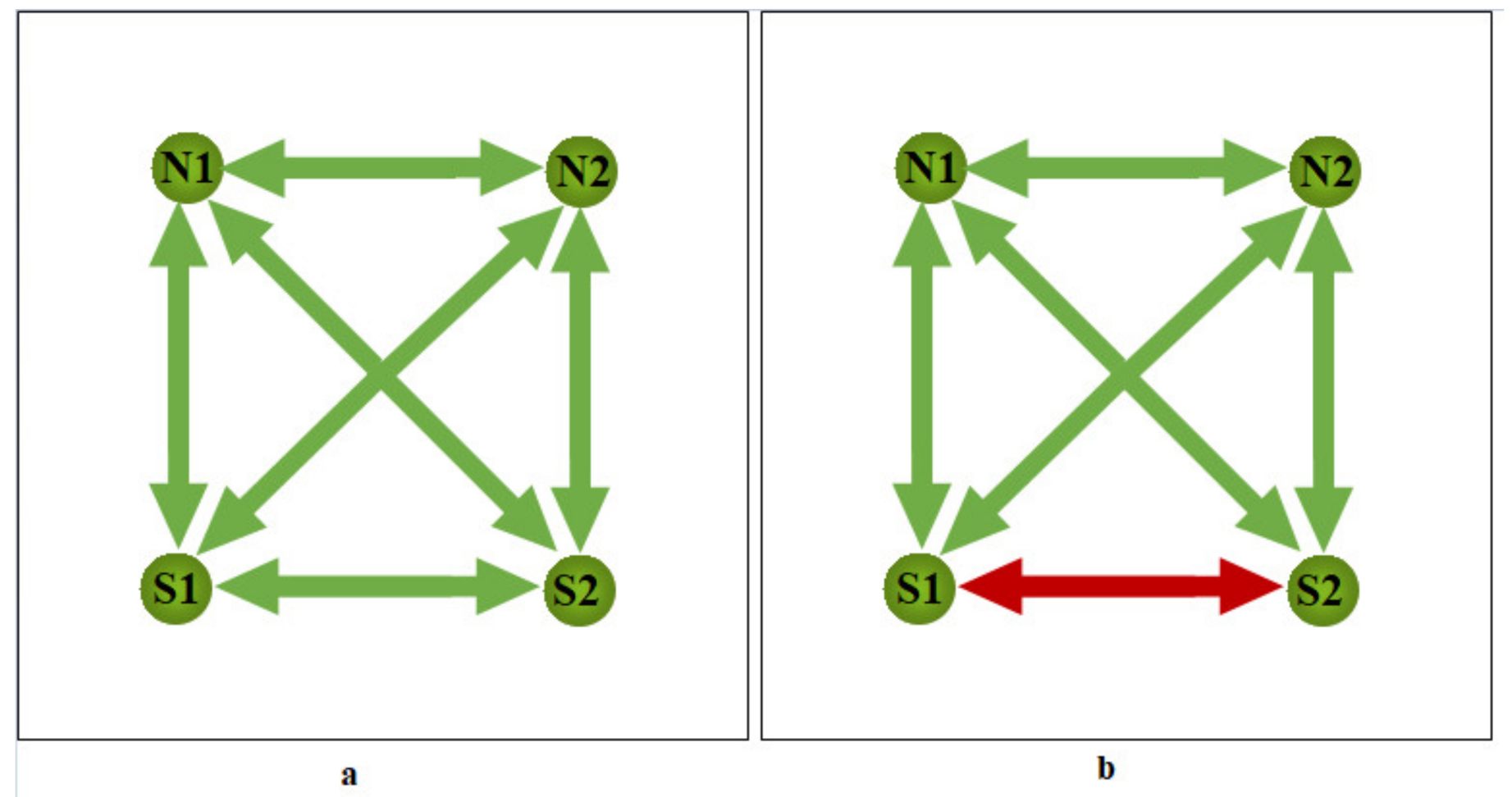
The ANOVA results in

Table 7. ANOVA results for T, RH, Tdp, VPD, SR, and CO₂ distribution in SLG. T: air temperature; RH: relative humidity; T_dp: dew point temperature; VPD: vapor pressure deficit; SR: solar radiation.

Parameter	df	F	p-Value	F Crit
T (°C)	8, 158,913	83.49	p < 0.01	1.94
RH (%)	8, 158,914	121.50	p < 0.01	1.94
Tdp (°C)	8, 158,915	132.53	p < 0.01	1.94
VPD (kPa)	8, 158,916	126.52	p < 0.01	1.94
SR (W/m2)	1, 13,168	2148.90	p < 0.01	3.84

and

Table 8. ANOVA result of the T, RH, T_dp, VPD, SR, and CO₂ distribution in DLG. T: air temperature; RH: relative humidity; T_dp: dew point temperature; VPD: vapor pressure deficit; SR: solar radiation.

Parameter	df	F	p-Value	F Crit
T (°C)	8, 158,913	97.73	p < 0.01	1.94
RH (%)	8, 158,914	45.51	p < 0.01	1.94
Tdp (°C)	8, 158,915	25.78	p < 0.01	1.94
VPD (kPa)	8, 158,916	108.89	p < 0.01	1.94
SR (W/m2)	1, 13,168	2066.50	p < 0.01	3.84

show the significant differences in the distribution of all the microclimate parameters within the greenhouses. The p-value corresponding to the F-statistic of one-way ANOVA is less than 0.05, indicating that one or more treatments are significantly different. Despite the installation of circulation fans in the greenhouses, the distribution was found to be heterogeneous. This significant variation supports the findings by [8], who stated that significant temperature gradients were observed even when experiments were conducted in small experimental greenhouses. Except for the fog cooling condition, the result is similar to the result obtained by [12], who reported nonuniformity of T and RH distribution within a conventional DLG during the day and nighttime, under heating, no heating, and no fogging conditions. However, [22] found no differences in T and RH readings between an SLG and DLG.

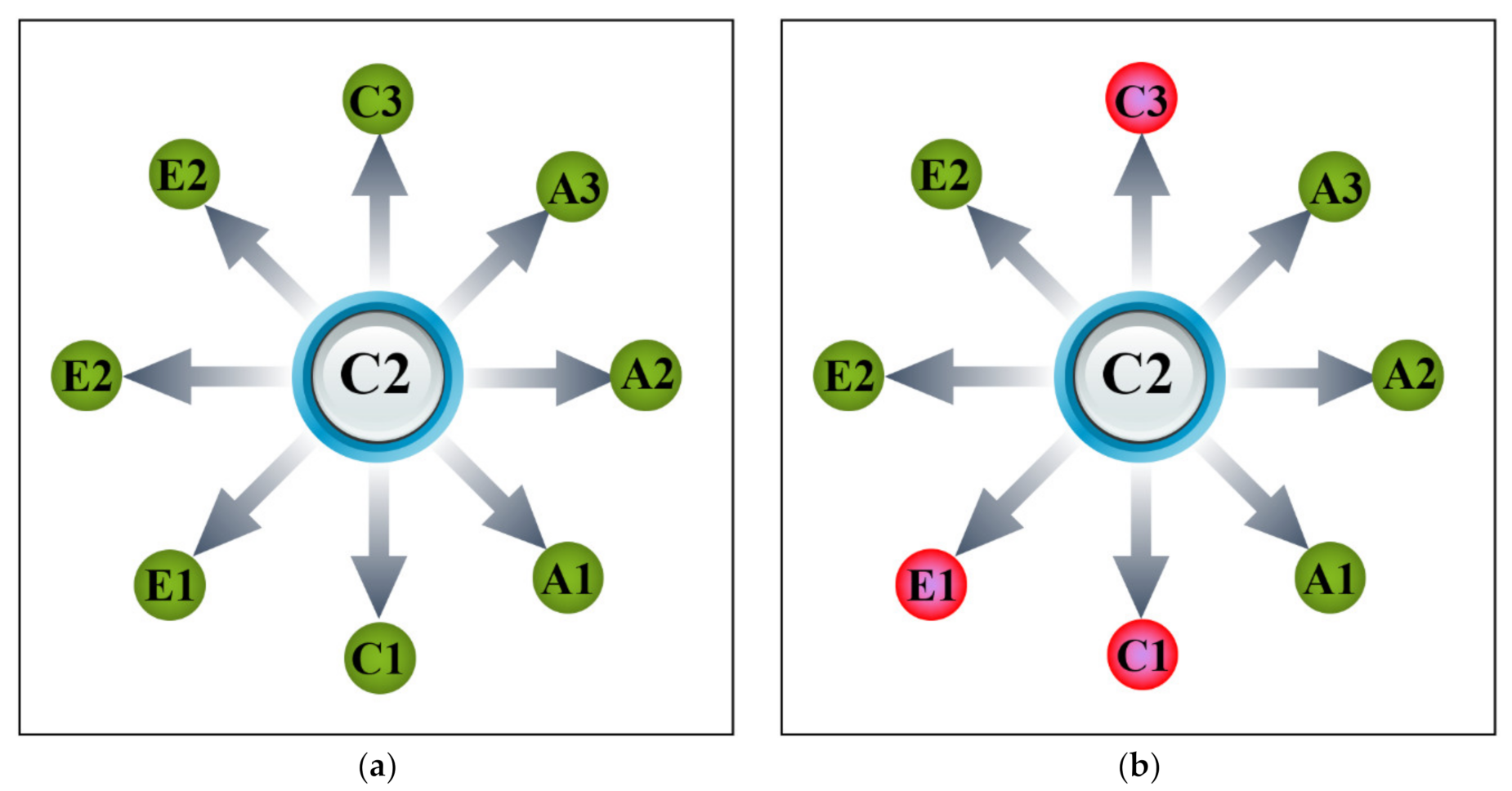
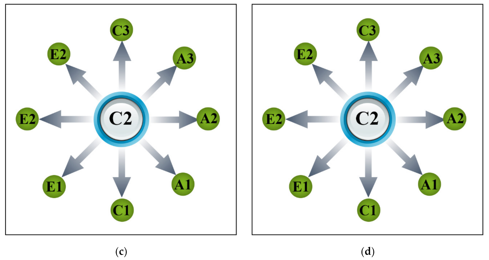
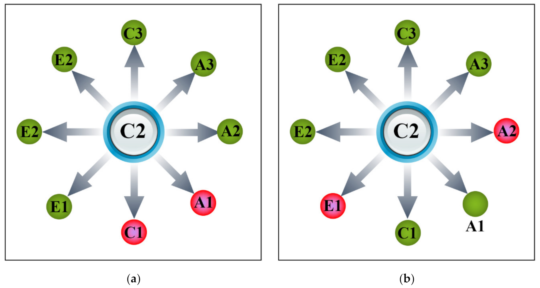
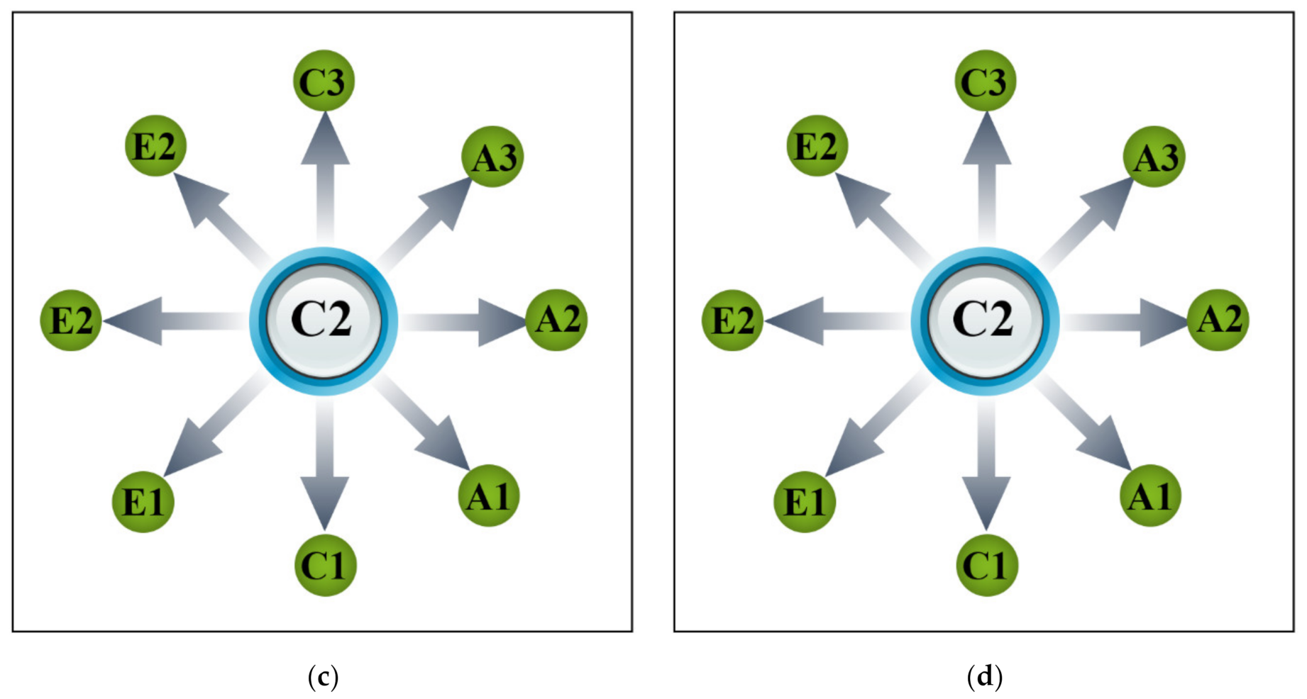
Figure 4 and Figure 5 show the Tukey HSD test of data from the control sensor (C2) and other sensors in the SLG and DLG. In SLG, T, T_dp, and the VPD readings in the control sensor were significantly different from the other sensors. The RH in the control sensor was significantly different from all other sensors except for C1, C3, and E1. Similarly, in DLG, the variables T_dp and VPD gathered in the control sensor were significantly different from those obtained in other sensors. The variables T and RH in the control sensor were significantly different from all the other sensors, except A1 and C1, and A2 and E1. Considering the Tukey pairwise comparison of all sensors, the variables T, RH, T_dp, and VPD were 66.6%, 72.2%, 72.2%, and 80.5% higher in SLG. When DLG is considered, the variables T, RH, T_dp, and VPD were 80.5%, 72.2%, 50.0%, and 86.1%, respectively, higher than the control sensors. These values confirm that the distribution of the variables is heterogeneous. Refs. [14,23] recommended ±0.75 °C and ± 3% of standard deviation for T and RH, respectively, for a homogeneous distribution. T and RH in SLG and DLG analyzed in this study, were 4.786 °C and 18.84%, respectively, and 4.911 °C and 21.71%. These values were higher than the recommended, confirming the heterogeneity of heat distribution in both greenhouses.

As shown in Table 7 and Table 8, the SR distribution within SLG and DLG was also significantly different. The SR variation can be attributed to the interruption by thermal screens inside the covering material and condensation [24].

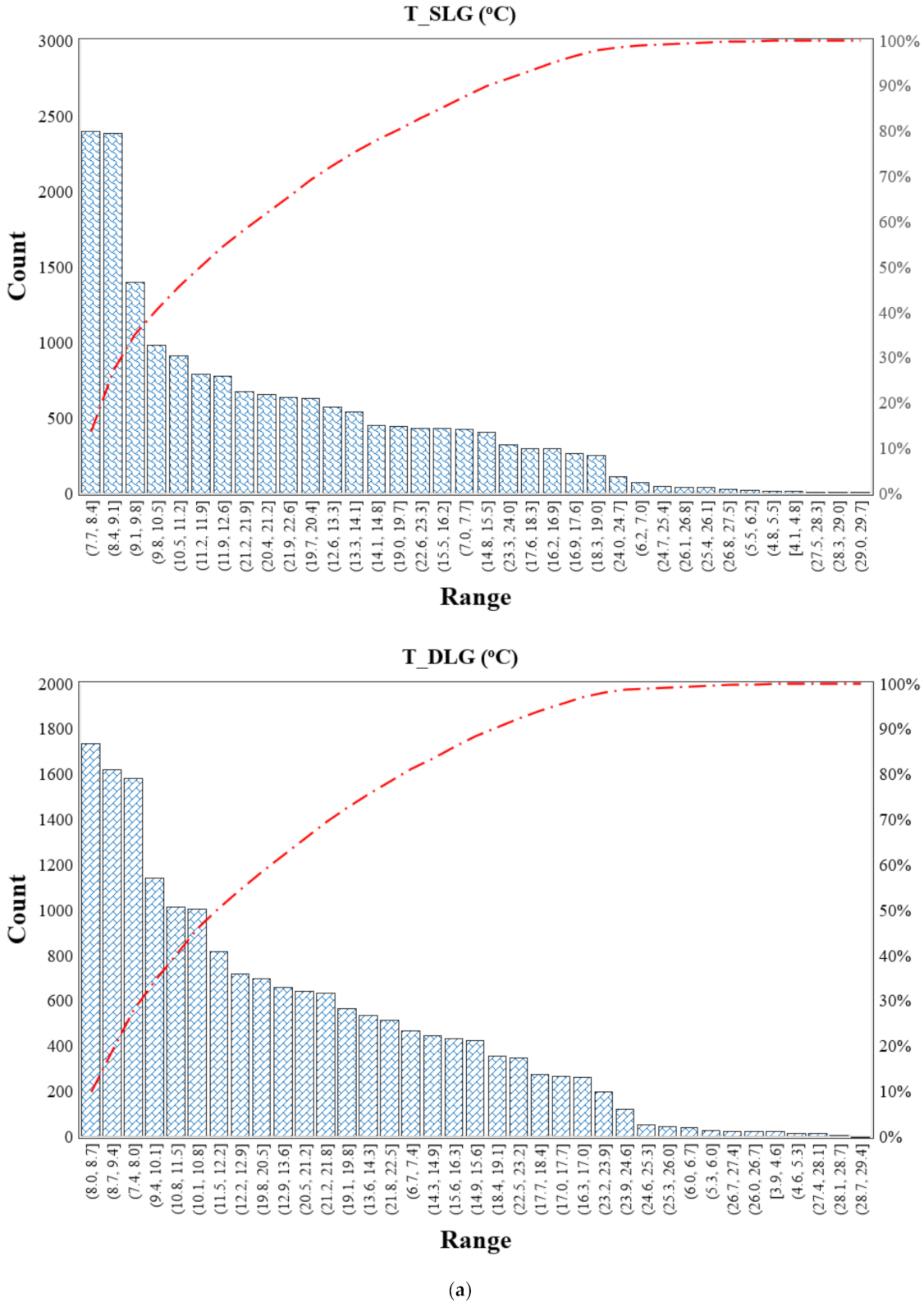
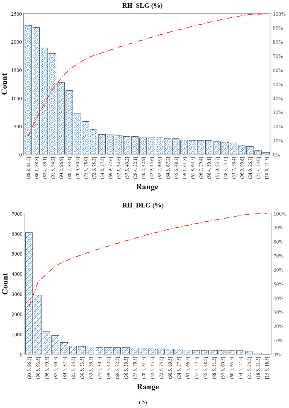
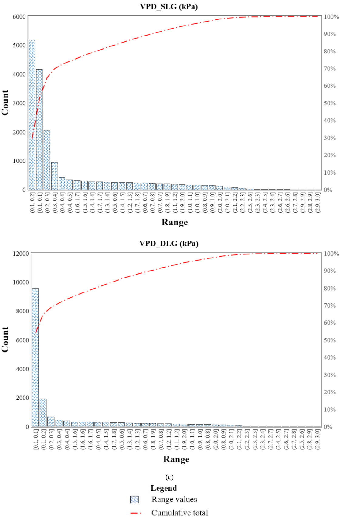
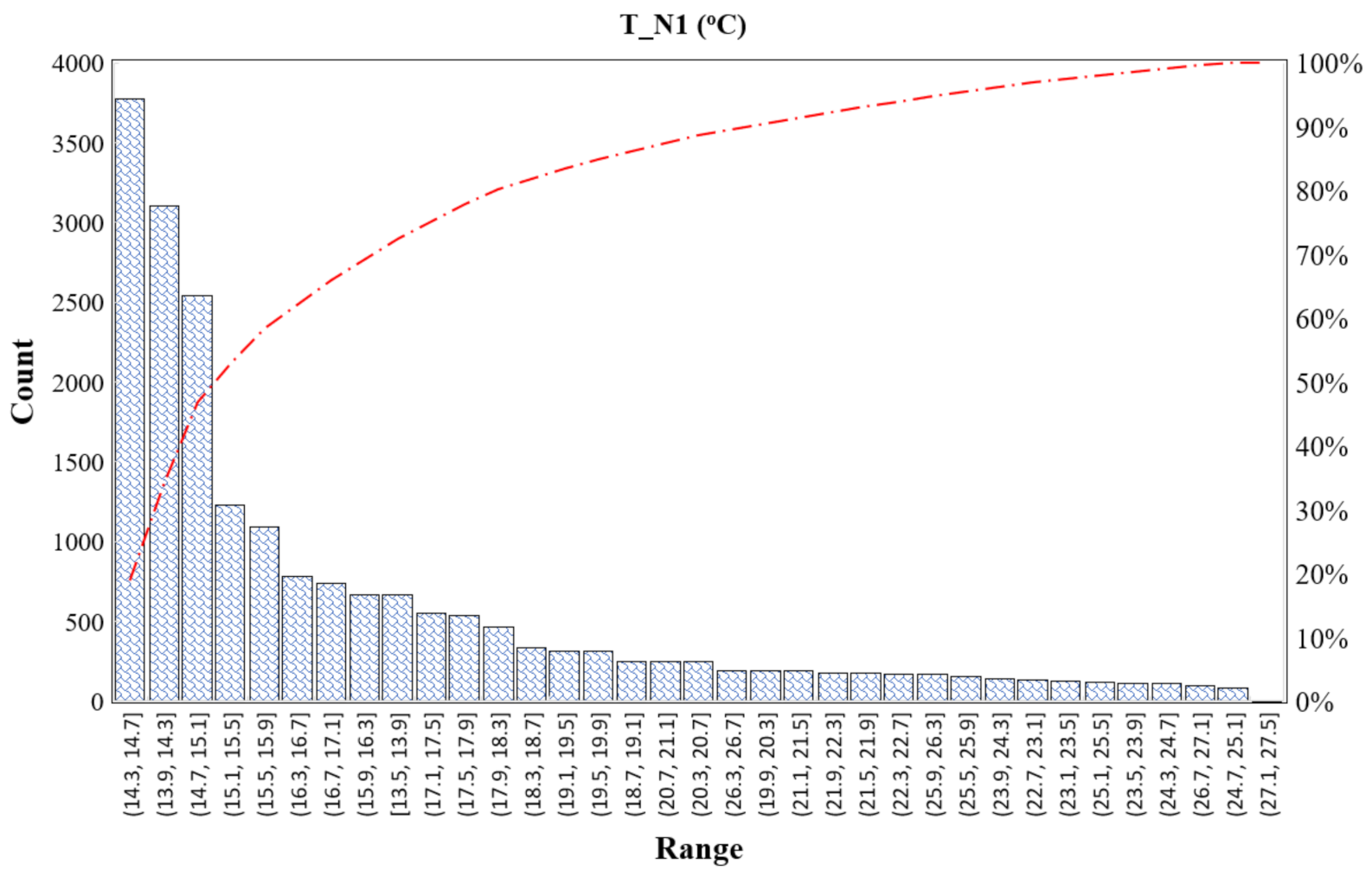
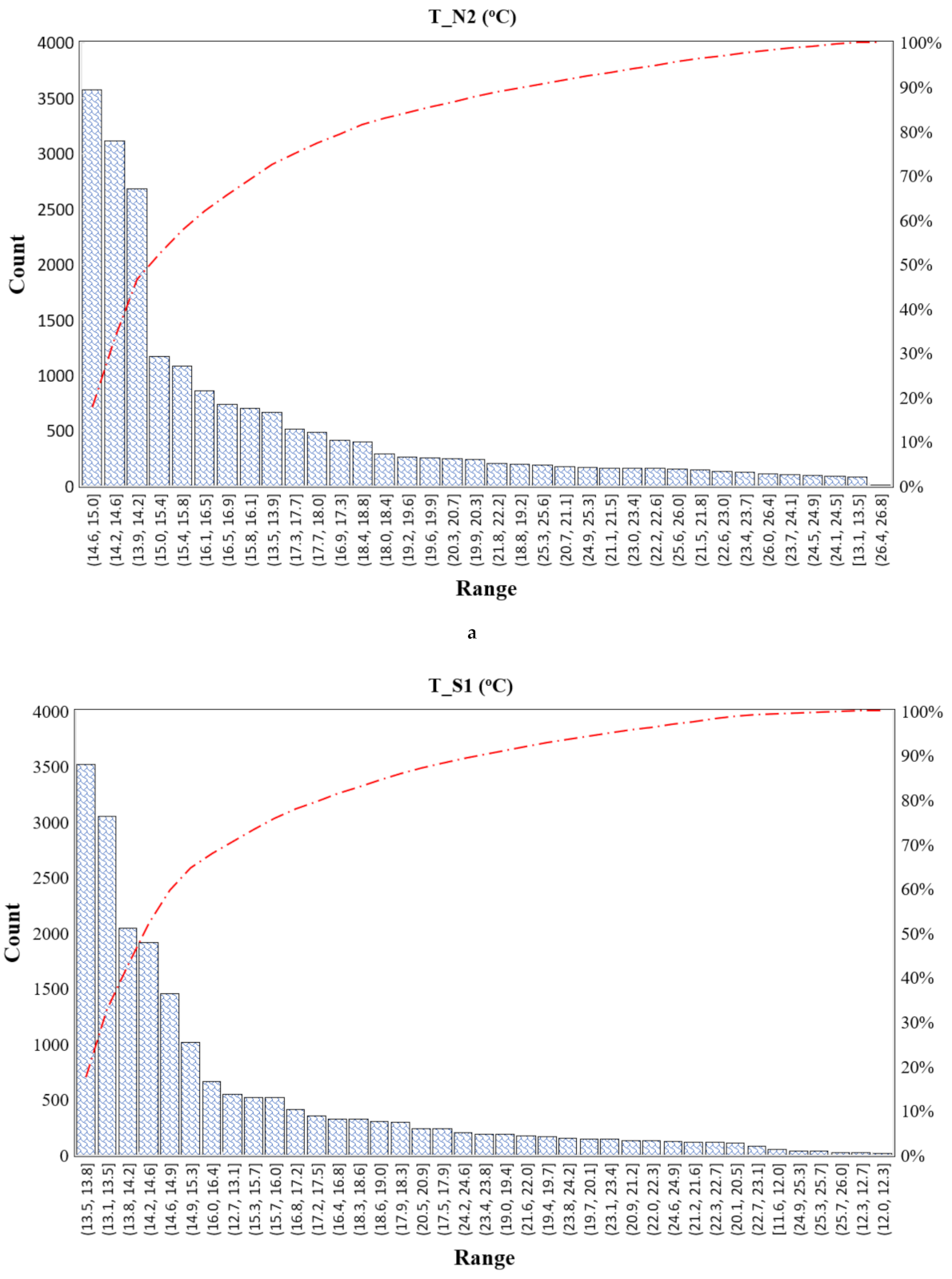
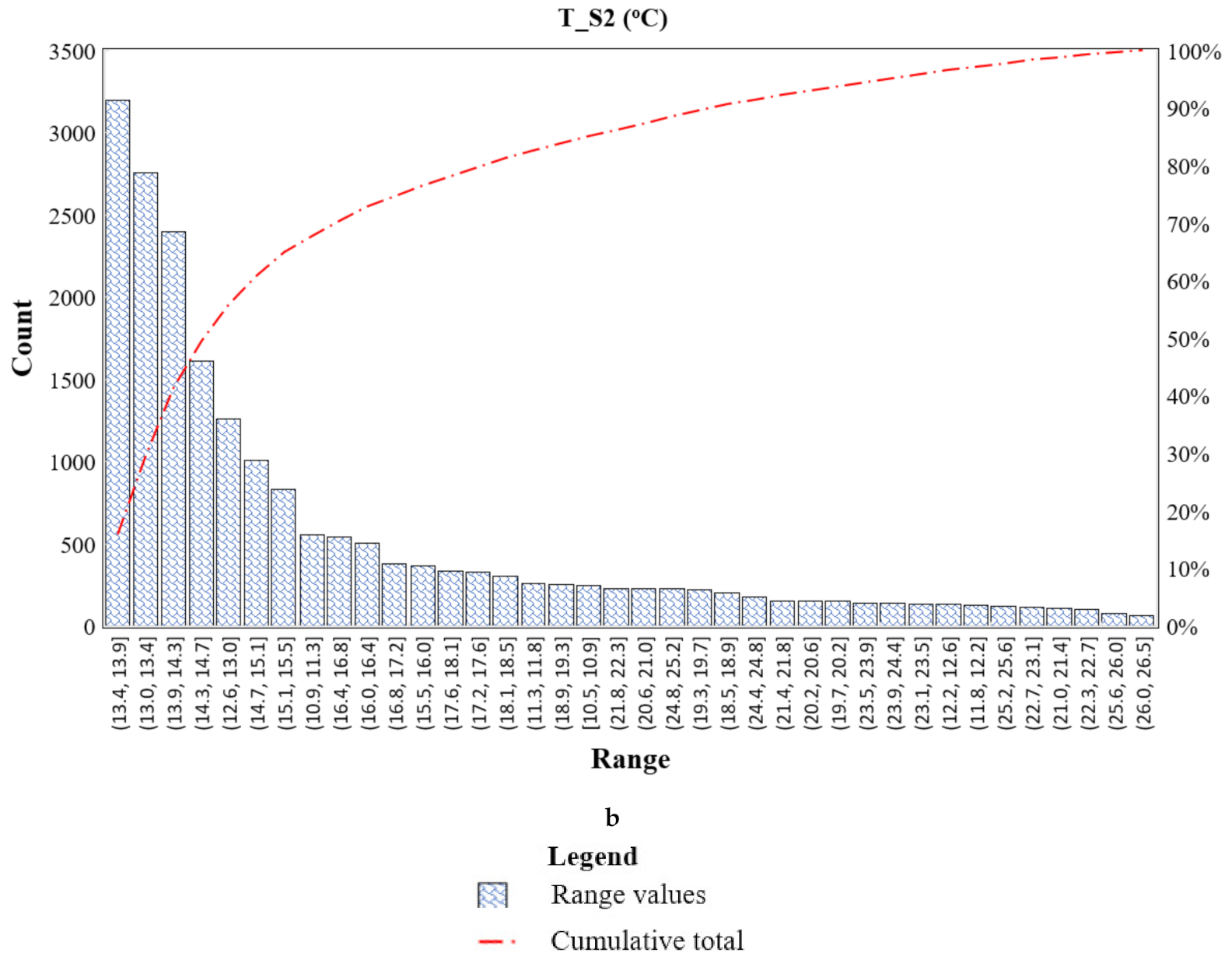
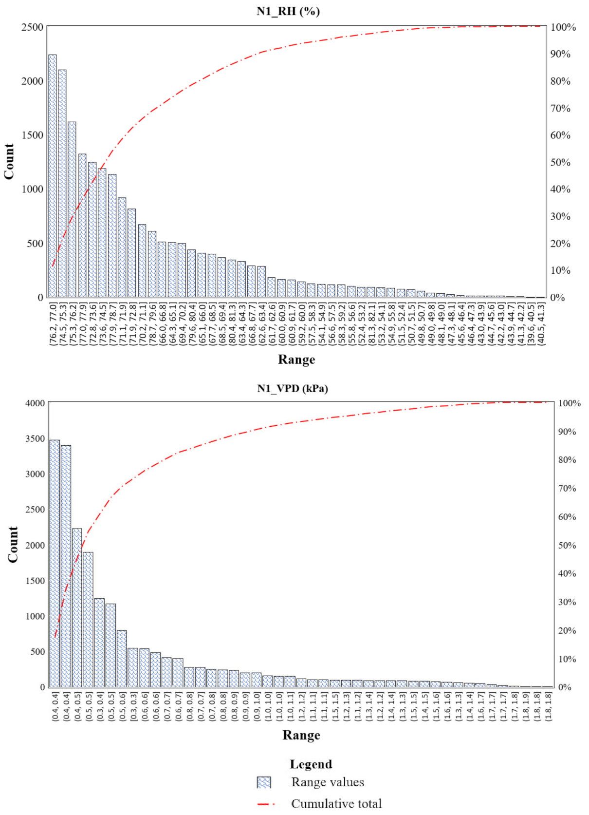
The Pareto chart in Figure 6 shows the distribution of T, RH, T_dp, and VPD data in the control sensors in SLG and DLG, respectively. In Figure 6a, the data for these variables in the SLG and DLG 8 were 95% and 94.2%, within the range of 8–23 °C; 40.4% and 40.06%, within the range of 7.3–10.8 °C; 17.1% and 20.0%, within the range of 10.9–13 °C; and, 22.6% and 22.7%, within the range of 18–23 °C. The minimum and maximum temperature setpoint in the SLG and DLG was 8–23 °C, respectively. However, for strawberries, refs [6,7] recommends optimum daytime and nighttime temperature ranges of 18–23 °C and 10–13 °C, respectively.

Figure 6b shows the RH data within the SLG and DLG were 10.7% and 10.4%, within the range of 60% and 75%; 20.5% and 19.2%, within 18–59% and 15–59% RH; and 68.7% and 70.3 %, within 76–96% and 76–99% RH, respectively. However, for strawberries, ref [4,6] recommend an optimum range of 60–75% RH. Figure 6c shows that the VPD data within the SLG and DLG were 21.2% and 10.2%, within the range 0.25 kPa and 0.5 kPa; 4.4% and 5.3%, within 0.8 kPa and 1.2 kPa, 9.1% and 7.8%, within 1.3 kPa and 1.6 kPa; 65.3% and 76.6%, were outside 0.2 kPa and 1.6 kPa in SLG and DLG, respectively. However, for strawberries, ref [4,6] recommended a range of 0.2–1.6 kPa.

Although 95% and 94.2% of the temperature data were within the setpoint range of 8–23 °C, respectively, approximately 68.7% and 70.3% of RH resulted in the VPD being outside the optimum value in SLG and DLG. The higher temperature sum at C2 than the temperature sums from other sensor points invariably means that the RH at these sensor points was higher. Therefore, this result means that the sensor readings will consequently result in lower VPD readings. Therefore, this result indicates worse conditions at other points.

3.1.2. Air-Leaf Temperature Interaction

During the day, there was a significant difference between the leaf and surrounding air temperature in both greenhouses, but only in SLG at night, as the p-value corresponding to the F-statistic of one-way ANOVA is less than 0.05, indicating that one or more treatments are significantly different. The ANOVA results for the air-leaf temperature in daytime and nighttime in SLG and DLG are shown in

Table 9. ANOVA results of the daytime and nighttime air-leaf temperature interaction in SLG and DLG. SLG: single-layered greenhouse; DLG: double-layered greenhouse.

Period	Interaction	df	F	p-Value	F Crit
Day	T_Leaf_SLG vs. T_Air_SLG	1, 35,998	122.48	p < 0.01	3.84
	T_Leaf_DLG vs. T_Air_DLG	1, 35,998	170.17	p < 0.01	3.84
Night	T_Leaf_SLG vs. T_Air_SLG	1, 35,998	17.44	p < 0.01	3.84
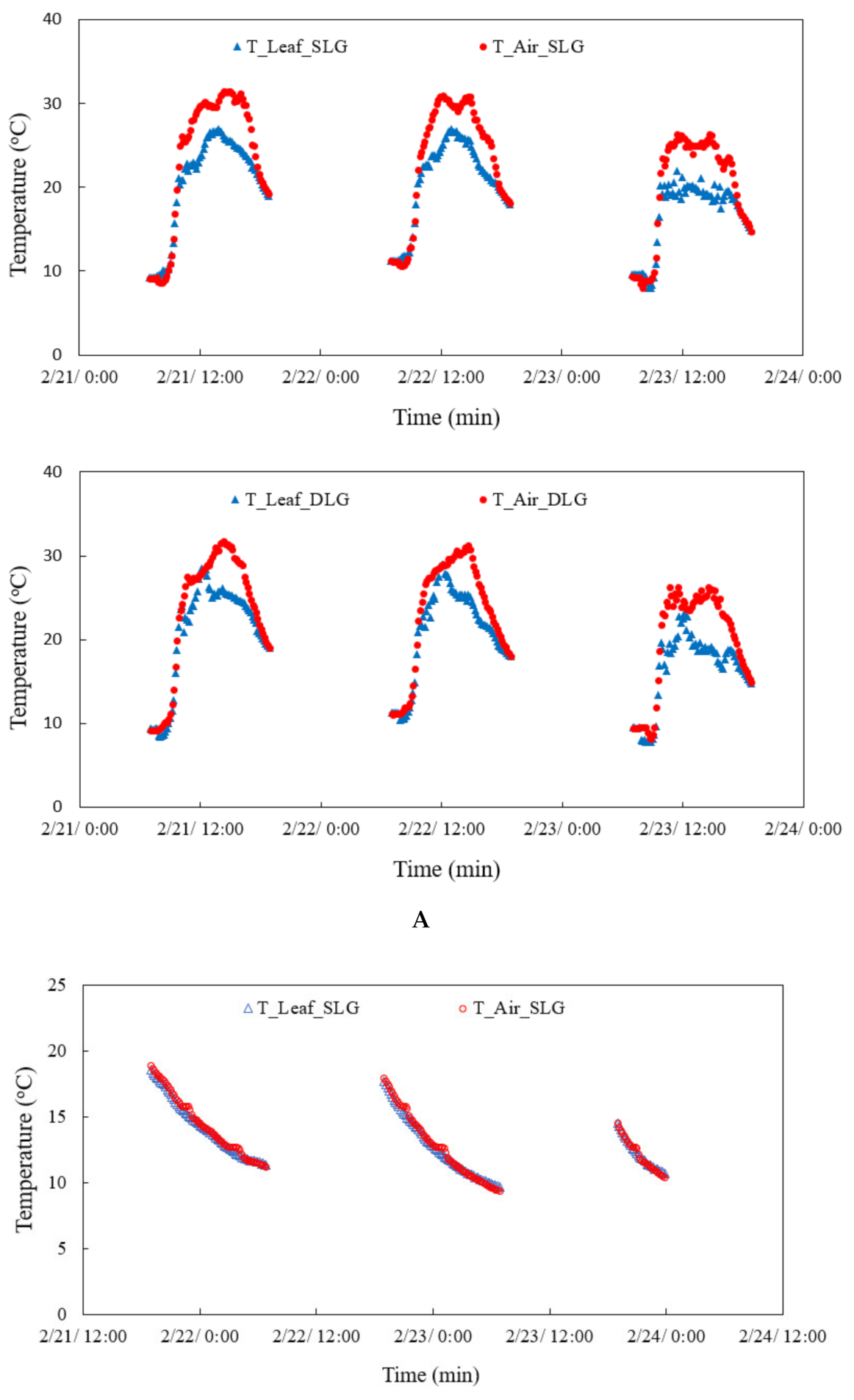
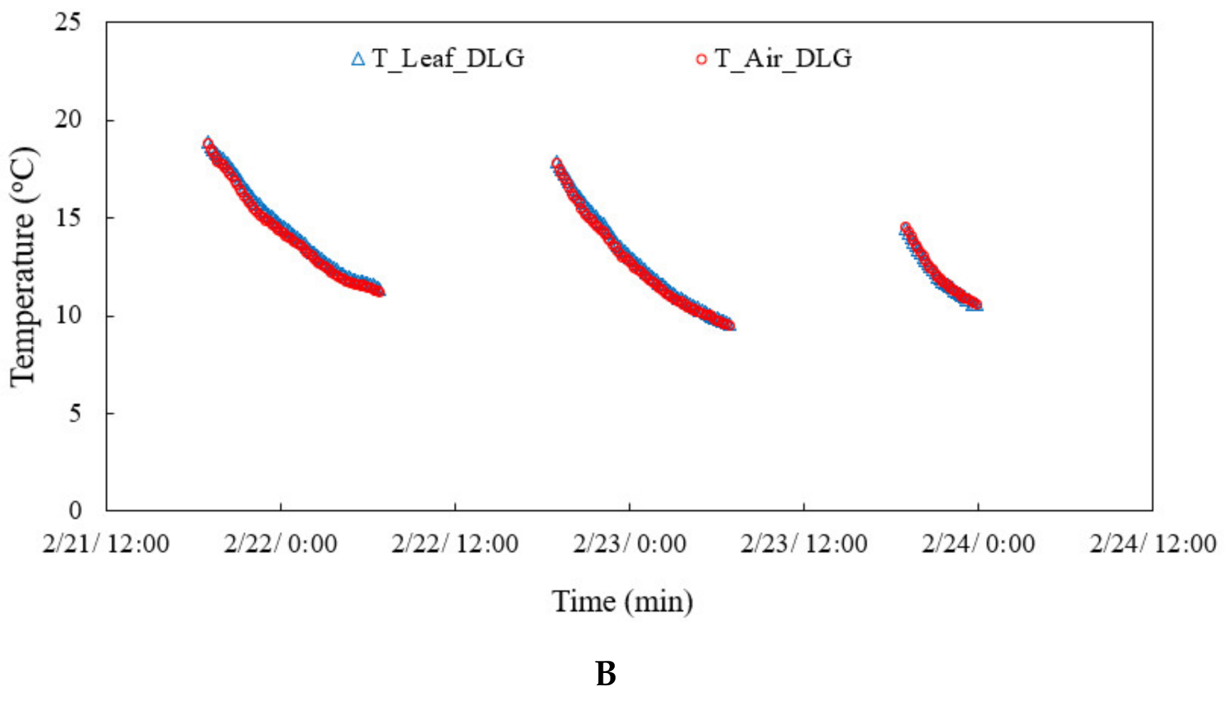
	T_Leaf_DLG vs. T_Air_DLG	1, 35,998	2.63	0.104787	3.84

, and the air-leaf temperature patterns in the daytime (Figure 7A) and nighttime (Figure 7B) are shown in Figure 7. During the day, as the thermal screen opens, the incoming SR warms up the microclimate environment increasing the air temperature. As the energy increases, so does the air temperature and the leaves, with both maintaining thermal equilibrium. As shown in Figure 7A, the rate of transpiration increased as crop temperature increased. The moisture evaporated from the leaf surface creates a cooling effect thereby reducing the leaf temperature. The crop behaved as a heat sink in those instances, resulting in energy loss because the air temperature was higher than the leaf temperature and to maintain thermal equilibrium with the surrounding air.

During the night, as the ambient temperature falls, energy is lost to the ambient because of the temperature difference between the greenhouses air temperature and the ambient temperature through the cover and infiltration. Figure 7B shows that as the air temperature falls, so does the temperature of the leaves. This is because of the exchange between the crop and the surrounding air. To maintain thermal equilibrium, the crop loses energy to the surrounding, as the greenhouse also loses energy to the ambient. This means that the greenhouse microclimate gains energy from the crop that subsequently loses it to the ambient environment. The leaf temperature was found to be higher than the air temperature at the late hours of the night and early hours of the day (Figure 7). This can be attributed to the energy gained through the crop root zone during the night from radiated heat from the heating pipe located beneath the root zone. When the greenhouse temperature falls below the set temperature of 8 °C, hot water is pumped through the pipes. The increase continued until the crop temperature exceeded the temperature of the surrounding air. During this period, the crop behaves like a heat source, emitting heat into the surrounding air, allowing the greenhouse microclimate to gain heat. This result is similar to that of [15], who reported similar crop and greenhouse air temperature trends. The implication of this is that, rather than the assumption of absolute heat loss reported by [3] and absolute gain reported by [25] to crop effect in energy estimation in a greenhouse, the TRNSYS building energy simulation crop model component that considers the changes in the air and crop temperature should be used.

3.2. Multi Span Greenhouse

Table 10. Descriptive statistics of T, RH, VPD, and CO₂ distribution in the fifteen-span greenhouse. T: air temperature; RH: relative humidity; T_dp: dew point temperature; VPD: vapor pressure deficit; SR: solar radiation; CO₂: carbon dioxide; N1, S1, N2, S2: experimental sensors; SD: standard deviation; Min.: minimum; Max.: maximum.

Parameter	Description	N1	S1	N2	S2
T (°C)	Mean	16.57	15.52	16.40	15.34
	Median	15.10	14.30	15.00	14.10
	Mode	14.40	13.50	14.80	13.70
	SD	3.11	2.91	2.96	3.25
	Min.	13.50	11.60	13.10	10.50
	Max.	27.20	26.00	26.50	26.40
	Sum	333,757.10	312,632.00	330,379.50	309,046.00
RH (%)	Mean	72.16	75.48	73.28	75.54
	Median	74.30	78.10	74.90	78.30
	Mode	77.00	80.00	77.30	79.80
	SD	6.62	6.65	5.67	6.90
	Min.	39.60	42.20	45.00	42.70
	Max.	82.00	83.10	83.40	83.20
	Sum	1,453,788.20	1,520,680.70	1,476,234.60	1,521,782.60
VPD (kPa)	Mean	0.55	0.46	0.52	0.46
	Median	0.45	0.36	0.43	0.34
	Mode	0.37	0.30	0.42	0.29
	SD	0.27	0.24	0.23	0.27
	Min.	0.29	0.26	0.26	0.23
	Max.	1.86	1.73	1.60	1.81
	Sum	11,164.09	9215.84	10,496.89	9212.35
CO2 (ppm)	Mean	526.85	533.91	592.75	452.15
	Median	502.00	521.00	576.00	439.00
	Mode	501.00	527.00	581.00	443.00
	SD	120.14	99.64	126.00	105.31
	Min.	267.00	288.00	304.00	207.00
	Max.	1156.00	1068.00	1083.00	900.00
	Sum	10,613,874.00	10,756,218.00	11,941,488.00	9,109,010.00
	Count	20,146	20,146	20,146	20,146

shows the descriptive statistics of the microclimate parameters distribution for all sensors. The minimum and maximum temperatures of 10.5 °C and 27.2 °C were recorded at S2 and N1, respectively. The amount of temperature at N1 was 8.0%, 6.7%, and 1.0% higher than S2, S1, and N2, respectively. The lowest and highest RH values of 39.60% and 83.240% were recorded at N1 and N2. The sum of RH recorded at S2 was higher than RH at N1, S1, and N2 by 4.6%, 0.7%, and 3.0%, respectively. The sum value of VPD at N1 was higher than VPD at S1, N2, and S2 by 21.1%, 6.3%, and 21.2%, respectively. The lowest and highest VPD values of S2 and N1 recorded 0.23 kPa and 1.86 kPa, respectively. The sum of CO₂ recorded at N2 was 12.5%, 11.0%, and 31.1 % higher than the total CO₂ recorded at N1, S1, and S2, respectively. The lowest and highest values of 207 ppm and 1156 ppm were recorded at S2 and N1, respectively.

Table 11. ANOVA results for T, RH, VPD, and CO₂ distribution in the fifteen-span greenhouse. T: air temperature; RH: relative humidity; T_dp: dew point temperature; VPD: vapor pressure deficit; CO₂: carbon dioxide.

Parameter	df	F	p-Value	F Crit
T (°C)	3, 80,583	817.20	p < 0.01	2.61
RH (%)	3, 80,583	1345.42	p < 0.01	2.61
VPD (kPa)	3, 80,583	727.29	p < 0.01	2.61
CO2 (ppm)	3, 80,583	5218.42	p < 0.01	2.61

shows that there are significant differences in the distribution of the microclimate parameters within the greenhouse based on the ANOVA results. The p-value corresponding to the F-statistic of one-way ANOVA is less than 0.05, indicating that one or more treatments are significantly different. The Tukey pairwise comparison of the sensors regarding temperature, RH, VPD, and CO₂ is shown in Figure 8. The Tukey pairwise comparison of the sensors in Figure 8a for temperature and CO₂ was significantly different p < 0.01 from each other, whereas there was a similarity between sensors at S1 and S2 for RH and VPD as shown in Figure 8b, confirming the heterogeneity in their distribution [8]. The standard deviation (pooled total) of 3.1 °C and 6.6% for temperature and RH, respectively, also confirms the heterogeneity of the distribution of the parameters within the greenhouse [14,23]. In a similar result, ref [19] reported significant daily temperature differences inside a 15-span and 18-span greenhouse.

Figure 9 shows the distribution of the T data from sensors in the MSG. The spread shows that 32.92%, 34.01%, 27.50%, and 20.07% of the data were within the greenhouse control temperature range of 15–19 °C; 17.04%, 15.82%, 12.57%, and 12.64% above the setpoints; and 50.01%, 50.04%, 59.92%, and 67.27% below the set points in N1, N2, S1, and S2, respectively. The majority of those values, 58.24%, 57.62%, 64.54%, and 60.73 % are within the 13.9–15.9 °C (14.40 °C) range in N1; 13.9–15.8 °C (14.8 °C) in N2, 13.1–15.3 °C (13.5 °C) in S1 and 12.6–15.1 °C (13.7 °C) in S2, respectively. As shown in Table 10, the bracketed values represent the mode of the data. These results indicate that the control sensor is in the vicinity of the N-zone. By implication, because of the heterogeneity of the temperature distribution, the conditions in other parts may be unfavorable to the crops.

The data spread for RH and VPD were considered only for N1 (Figure 10) because it falls within the N-zone. With the minimum and maximum RH being 39.60% and 82.00%, respectively, 38.70% of the data was within the range 75–82% of RH, and 54.66% was within the range 60–75% RH. However, [4,6] recommended an optimum RH range of 60–75%. In this case, 94.15% of the VPD data were within the recommended value of 0.2–1.2 kPa for strawberry, whereas 54.05% was below 0.5 kPa [4,5]. These results show an optimum condition at the point despite 32.92% of the temperature data failing within the temperature setpoint. Contrary to the result in the SLG and DLG, where all data falling within the setpoints resulted in the VPD being outside the optimum range, approximately 33% of the temperature data in MSG falling within the setpoints resulted in the majority of the VPD data falling within the optimum range. The implication of this is that it will be beneficial for the crop if VPD is used as a setpoint rather than the temperature.

4. Conclusions

Heat and mass distribution variations in single- and MSGs were statistically analyzed. Analyses showed significant variations in the horizontal distribution of T, RH, SR, CO₂, and VPD within the single- and multi-span greenhouses despite the installation of distribution fans in the greenhouses. Unlike the vertical variation in greenhouses, where the temperature difference between the top and bottom of the greenhouse is approximately 4–6 °C, and horizontal variation in an unfanned greenhouse, where the difference is approximately 3.5 °C, the difference between the center and the side into the single-span was approximately 0.88–1.0 °C, and in the MSG was approximately 1.03 °C.

Because the crops are arranged horizontally, the overall Tukey pairwise comparison of the variable sensors of 50–86% indicates that the majority of the crop was never in the same condition. While some are growing well, others may be exposed to diseases because of high VPD value or tip burns due to low VPD value.

There is a significant variation between the central and side’s sensors. The variation between the central and sides sensors was expected because it is easier to lose energy from the sides than the center, which is far from the ends. However, the result also showed variation between the sensors of both sides. This is because when the side vents are opened during the day, the amount of wind for ventilation will be different due to the orientation of the sides to the wind direction. Furthermore, external obstructions redirect the wind and cast shade.

In greenhouse control, using a single temperature value as the setpoint does not accurately represent the condition within the greenhouse. Therefore, further research should be conducted using VPD as the control and energy demand estimation parameter.

This study result will help in making the following decisions: (a) where the temperature sensors (which control the heating system operation) should be positioned and (b) what should be the setpoint temperatures knowing that different temperatures will exist within the greenhouse. Additionally, the last one may finally lead to alteration of the predicted energy consumption.

The use of energy simulation tools such as TRNSYS to estimate the energy demand of greenhouse can be conducted more accurately by considering the distribution of the microclimate parameters required as input in the model. Using this method, underestimation or overestimation can be avoided. Furthermore, the TRNSYS model can make use of the crop component model that considers instant changes in the air and crop temperature.