1. Introduction
Full attention to the increasing worldwide demand for food due to a growing human population [
1] is critical for securing current and future needs; these issues will be solved by increasing crop yield as a high priority, where the two key targets to focus on are genetic- and agronomic-based improvements. Traditional breeding methods are based on pedigree and phenotypic information for selecting superior cultivars to achieve increased genetic gains [
2,
3]. However, field phenotyping all of the genotypes derivable from all potential crosses is unfeasible. The use of DNA (deoxyribonucleic acid) sequence information offers a practical means for predicting the performance of candidate genotypes using the commonly called GP (Genomic Prediction) models, which then can be implemented in genomic selection (GS) schemes. GS is an emergent methodology that has the potential to significantly increase genetic gains by shortening breeding cycles and improving the accuracy of selection.
Genomic selection is an excellent tool for selecting genotypes during the early phases of the breeding pipeline [
4]. For example, Meuwissen et al. [
5] proposed a set of GP models for animal breeding that would cope with the burden of fitting models with relatively high-dimensional genomic covariates. GP requires both phenotypic and genotypic information to enable the calibration of the prediction models to predict the performance of non-phenotyped genotypes using only their DNA marker profiles. Hence, GP leverages the genomic relationships between phenotyped and non-phenotyped individuals by using genome-wide markers for computing genomic estimated breeding values (GEBVs) of unobserved genotypes [
6,
7]. Then, the GEBVs are used as phenotypic surrogates that breeders can consider when assessing performance relative to the selection of superior genotypes.
The application of GP plays an important role in plant and animal breeding programs when considering complex traits (i.e., traits affected by many genes with small effect) [
8,
9]. For most post-harvest traits of interest (i.e., yield, seed number and size, seed oil and protein, etc.), the focus of selection is typically on the favored right or left tail of the distribution of the predicted GEBVs. However, when the traits of interest have an intermediate distributional optimum, the fractional tail-specific selection is not applicable [
10]. These situations are often found when one considers pre-harvest crop phenotypes of interest, such as the dates of flowering and/or maturity (in soybeans the occurrence of DTM (days to maturity) is denoted as R8), which are typically measured as days after the date of planting (or emergence).
For these time-related traits, the per se GEBVs are more important than their relative ranking, primarily because crop phenology is a major element in the adaptation of a crop species within the current targeted production environments, as well as any potential expansion of the crop to non-contiguous (but suggestive) environments located elsewhere. Thus, the implementation of GP models for predicting time-related traits must be carefully considered or it could lead to a misadjustment of the crop developmental sequence, a misclassification of genotypes for local adaptation, or an admixture of these two problems.
Soybean plant physiology and its relationship with crop phenology were recently reviewed [
11]. Soybean plant development consists of vegetative (V) and reproductive (R) phases that overlap in the indeterminate cultivars grown in the northern USA, but these phases are more distinctly separated in the determinate cultivars grown in Southern USA. Most soybean researchers use the soybean vegetative (Vn) and reproductive (Rn) staging system developed by [
12]. In that system, main stem nodes are assigned a cumulative number n, beginning with zero (V0) for the opposing two cotyledonary nodes, one (V1) for the opposing two unifoliolate leaf nodes, and two (V2) and up for each subsequent alternating trifoliolate leaf node (for Vn details and photos, see pp. 43–52 in [
13]).
The reproductive phase begins with stage R1, which is when the first open flower appears on the main stem. However, floral induction begins earlier (R0) when the unifoliate leaflets appear at stage V0 [
14]. These initial leaflets (plus all subsequent ones) sense and measure the dusk-to-dawn night length. If long enough (the duration of which is genotype-dependent), those leaflets will produce florigen, which is then transported via the phloem to the apical meristem located at the main stem tip (and branch tips), as well as to the lateral meristems located in each stem (and branch) leaf axil [
15]. Upon arrival, the florigen immediately induces the conversion of vegetative meristems (those not yet committed to becoming branches) to an inflorescence meristem that produces flowers.
Floral induction is essentially driven by the photoperiod, but the subsequent floral evocation (leading to visible floral buds and open flowers) is essentially temperature-driven. For Midwestern USA cultivars spanning maturity groups (MGs) 3.0 to 3.9, ref. [
16] documented a 28–32-day timeframe from V1 to R1, irrespective of planting dates that had been staggered at two-week intervals. This suggested that the calendar date of R1 (first flower) was quite predictable based on cultivar MG, production site latitude (i.e., photoperiod), and the date of V0 or V1. In the absence of seasonal water stress, the Vn and Rn stages are also potentially predictable with soybean crop models [
17].
The SoySim model was developed for Vn and Rn prediction in indeterminate cultivars of MG I, II, III, and IV that are grown in the Northern USA [
18] when the model is supplied with virtual day-by-day photoperiod and temperature data. After flowering begins at R1 and proceeds to full bloom (R2), stage R3 begins when pods emerge from pollinated flowers and elongate to a full length (R4), after which stage, R5 begins when seeds form in the pods and seed-filling commences until the seeds fill their pod cavities (R6). Stage R7 (at least one mature pod per plant) is defined as
physiological maturity, which is coincident with the cessation of plant photosynthetic activity (i.e., abscission of most, if not all, of the main stem nodal leaves). A key final soybean development stage is R8, which is when 95% of the pods borne on plants of a given genotype have attained a final mature color of brown or grey, after which, combine-ready harvest can occur when the in-field seed moisture falls to 13% (for Rn photos and details, see pp. 53–64 in [
13]).
Soybean crop V and R phasic progress towards maturity is dependent on genetic and environmental factors that are essential for crop adaptation, and thus, is critical regarding the breeder-mediated selection of advanced breeding lines that need to be evaluated in properly chosen latitudinal production environments. Soybean breeders are interested in the measurement of the number of days from planting to R8, termed days to maturity (DTM), because it characterizes what photoperiodic latitude is likely to have an adaptive fit. In the northern hemisphere, there are 13 MGs, numbered from 000 (very early) to X (very late), with extreme MGs typically grown in high and low latitudes, respectively [
19], though a 14th MG of 0000 was recently proposed. A similar 13th MG numbering scenario from low to high latitudes is used in the southern hemisphere [
20].
Soybean breeders maintain tight control over maturity during selection by evaluating breeding lines whose harvest maturity (R8) must be aligned with a given standardized MG latitudinal zone. The latter is defined empirically by using well-tested early and late cultivar checks to bracket the 8- to 10-day period of R8 dates in high latitude temperate zones but a wider period (15–20 days) in lower latitude tropical regions of each given MG zone [
20,
21]. Breeding lines undergo many within-state performance trials involving comparisons with existing cultivars of known MG so that the R8 data for those lines can be used to assign an MG decimal number (X.X) to the most advanced breeding lines that are worthy of cultivar release, thus denoting their latitudinal area of adaptation.
It would be useful to predict an R8 date (or more specifically, the number of days from planting to R8, which is DTM) for any given existing breeding line for one or more production sites in which that line was never tested, assuming that the given line or its relatives had been tested at other sites. Given that production sites of a similar latitude would experience a similar (predictable) photoperiod, DTM prediction is possible if that photoperiod can be used in GP schemes. This was documented to be successful when used to predict the heading date in rice (
Oryza sativa) [
10], but it has not yet been demonstrated in soybean (
Glycine max).
The advancements in sequencing technologies offer the opportunity of studying these traits from a different approach that considers causal relationships between genes and growth stages. It is well-known that molecular mechanisms play an important role in flowering time and maturity, with these two stages being the result of complex traits composed of multiple genes. Flowering and maturity time in soybean are controlled by the major E genes (they explain most of the variation in the number of days for soybean crops to achieve maturity) and these major E genes possess various functions regarding maturity and photoperiod sensitivity [
22]. Furthermore, their allelic variation and combinations can define the diversification of the soybean maturity groups and the adjustments to diverse latitudes [
23].
Currently, 11 major E loci (E1–E10 and J) were identified and classified through QTL mapping studies [
22,
24]. In addition, Wang et al. [
25] identified the gene E11 as a promoter of the flowering time and maturity. Recently, Zhang et al. [
26] found that soybean cultivars carrying the e1-as/e2-ns/E3-ha/E4 haplotype flowered earlier (7.6 days) than the flowering haplotype E1/e2-ns/E3-ha/E4. The major E genes (E1–E4) were deeply analyzed to understand the process of flowering time and maturity [
27]. For instance, the major genes E1 and E2 were described by Bernard [
28], and these were linked to controlling the flowering time and maturity. Kilen and Hartwig [
29] found that the E3 gene is related to late flowering, and Buzzell and Voldeng [
30] concluded that the gene E4 presented late flowering and sensitivity to prolonged daylength. Miranda et al. [
31] studied soybean lines in different environments for characterizing days to flowering, days to maturity, and plant height based on allelic combinations. Their results showed that the mutant gene J and the E1 gene influenced days to maturity and days to flowering. However, further studies are necessary for effectively connecting these parameters with markers or genes in prediction models.
Usually, multi-environment trials are established to study the local adaptation of plant cultivars to different locations. In many cases, the local adaptation depends on time-related traits, such as days to flowering or days to maturity. However, due to resource (land, water, phenotyping costs, etc.) constraints, it is not feasible to observe all genotypes in all environments, nor sample all the environments of interest. In general, the definition of environment is understood as the year × location combination; however, different sowing dates may also determine different environments, switching the definition of environment to the year × location × sowing date combination. The objective of this research consisted of developing and testing similar methods to those proposed by [
10] to accurately predict time-related traits in soybeans, such as days to maturity (DTM), in unobserved environments. For this, we considered the phenotypic and genomic information available from the SoyNAM experiments.
2. Materials and Methods
2.1. Phenotypic and Genotypic Data
For this study, we used genotypic and phenotypic data generated in the SoyNAM project, which were available from the SoyBase website (
https://www.soybase.org/SoyNAM accessed on 29 March 2022). More explicit details about the SoyNAM project were provided by [
32,
33]. Briefly, the SoyNAM project consisted of the development of 140 F5-derived recombinant inbred lines (RILs) from each mating of 40 soybean cultivars belonging to high-yielding lines (17, group 1), lines with diverse ancestry (15, group 2), and plant introductions with high yields in drought (8, group 3) to a common high-yielding hub parent (IA3023).
The 5600 NAM RILs were performance tested in 2011 (NE and IL locations only), then in 2012 and 2013 at nine locations in the US North-Central Region (for a total of 18 environment location × year combinations). Aside from the agronomic data, R8 dates were recorded at all sites. The NAM parents and RIL genotypes were sequenced with a 6k array, delivering a total of 5300 maker SNPs. After applying conventional quality control (discarding those molecular markers with more than 50% of missing values and a minor allele frequency smaller than 3%), 4300 SNPs were available for the analysis.
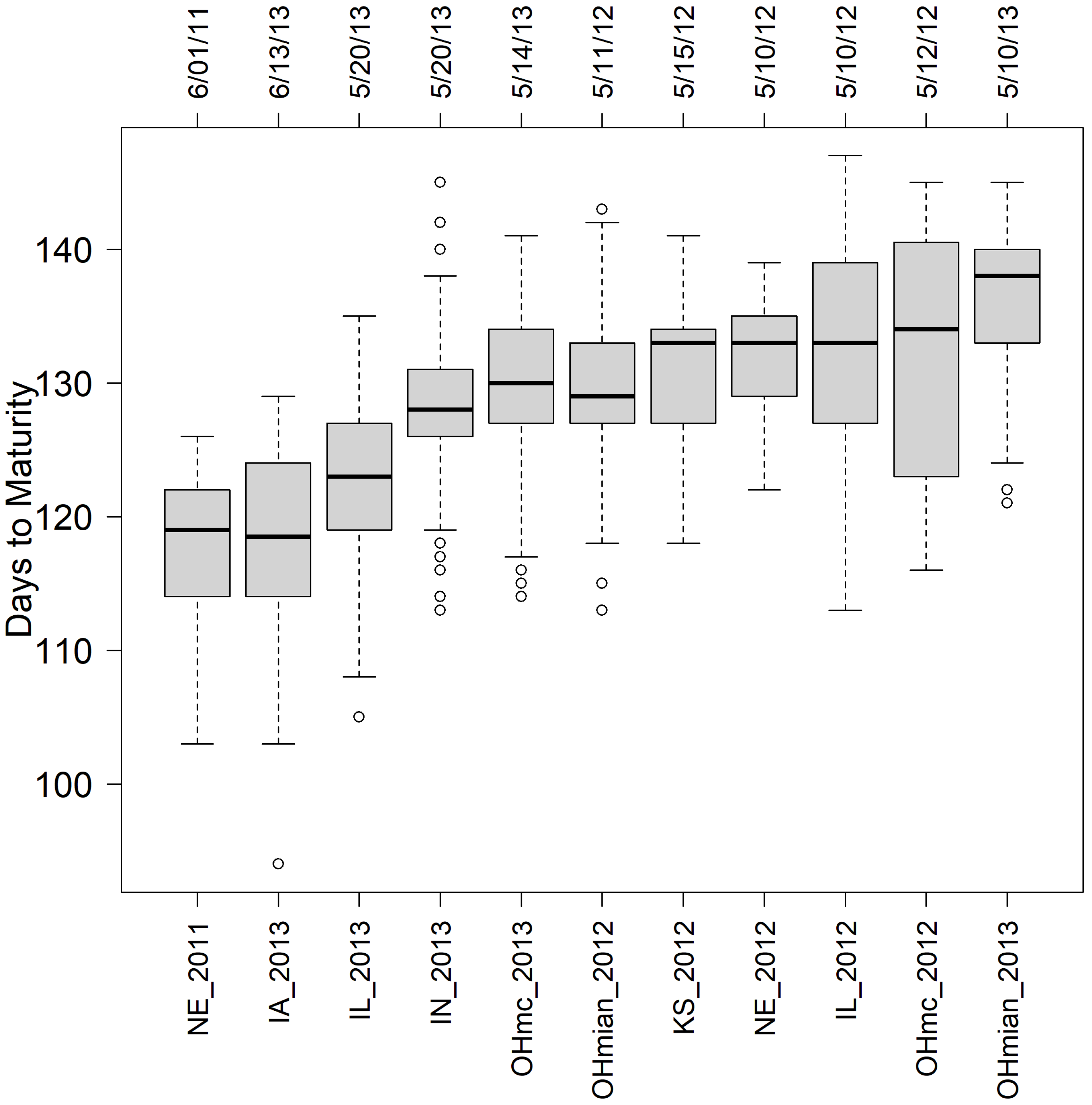
In this study, extra care was taken to have enough information for model calibration; thus, only those genotypes observed in at least 9 out of 11 preselected environments (those with the larger number of tested genotypes) were considered. Then out of the initial 40 families, 13 were randomly selected, with 7 belonging to group 1, 2 to group 2, and 4 to group 3, for a total of 367 RILs tested in 11 environments (NE_2011 [367], IL_2012 [367], NE_2012 [367], KS_2012 [337], OHmain_2012 [270], OHmc_2012 [127], IA_2013 [367], IL_2013 [367], IN_2013 [367], OHmain_2013 [206], OHmc_2013 [161]). The trait of interest for our study was DTM, which was derived for each location from the days between the site planting date and the RIL R8 date.
Table S1 in the Supplementary Materials provides the list of all genotypes in environments observed and their corresponding DTM. Moreover, the SNPs data corresponding to the 367 genotypes can be found in the
supplemental section (“SNPs.csv”). In addition, the population structure of the selected genotypes using the first two principal components was computed and is depicted in
Figure S1.
2.2. Daylength Data
Daylength was defined as the duration (time) of solar radiation from dawn to dusk. The daylength information of any site at any time of the year can be determined in advance by knowing the latitude of the location. Still, for the daily daylength during a soybean growing season, one must know the planting date (or date of V0/V1, when the photoperiodic floral induction begins). The daylength information used in this study was calculated with the model proposed by [
34], which is included in the geosphere (v1.5–5) R package. This package computes the theoretical daylength values based on the latitude, longitude, and planting date at each location.
2.3. Cross-Validation Schemes
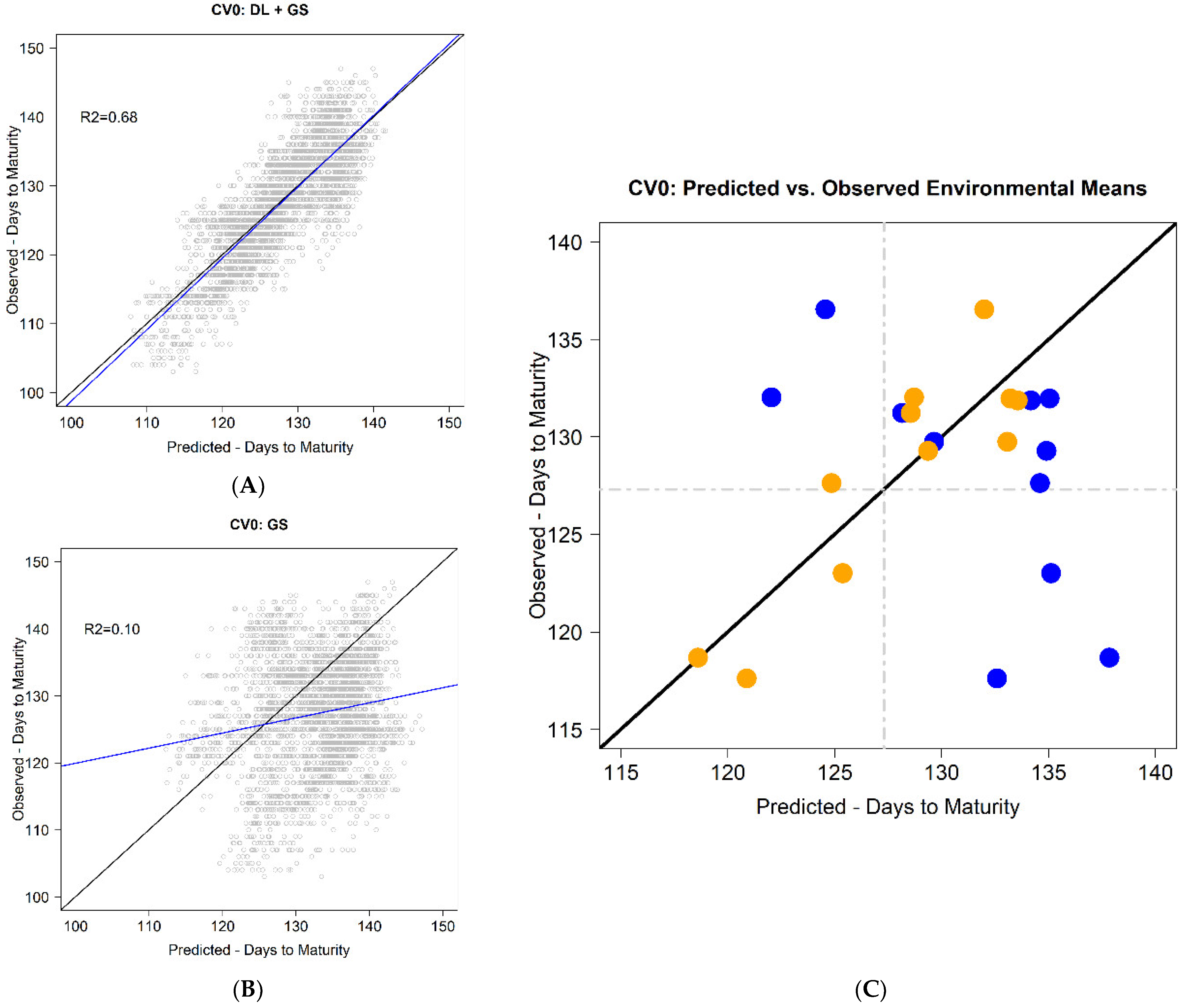
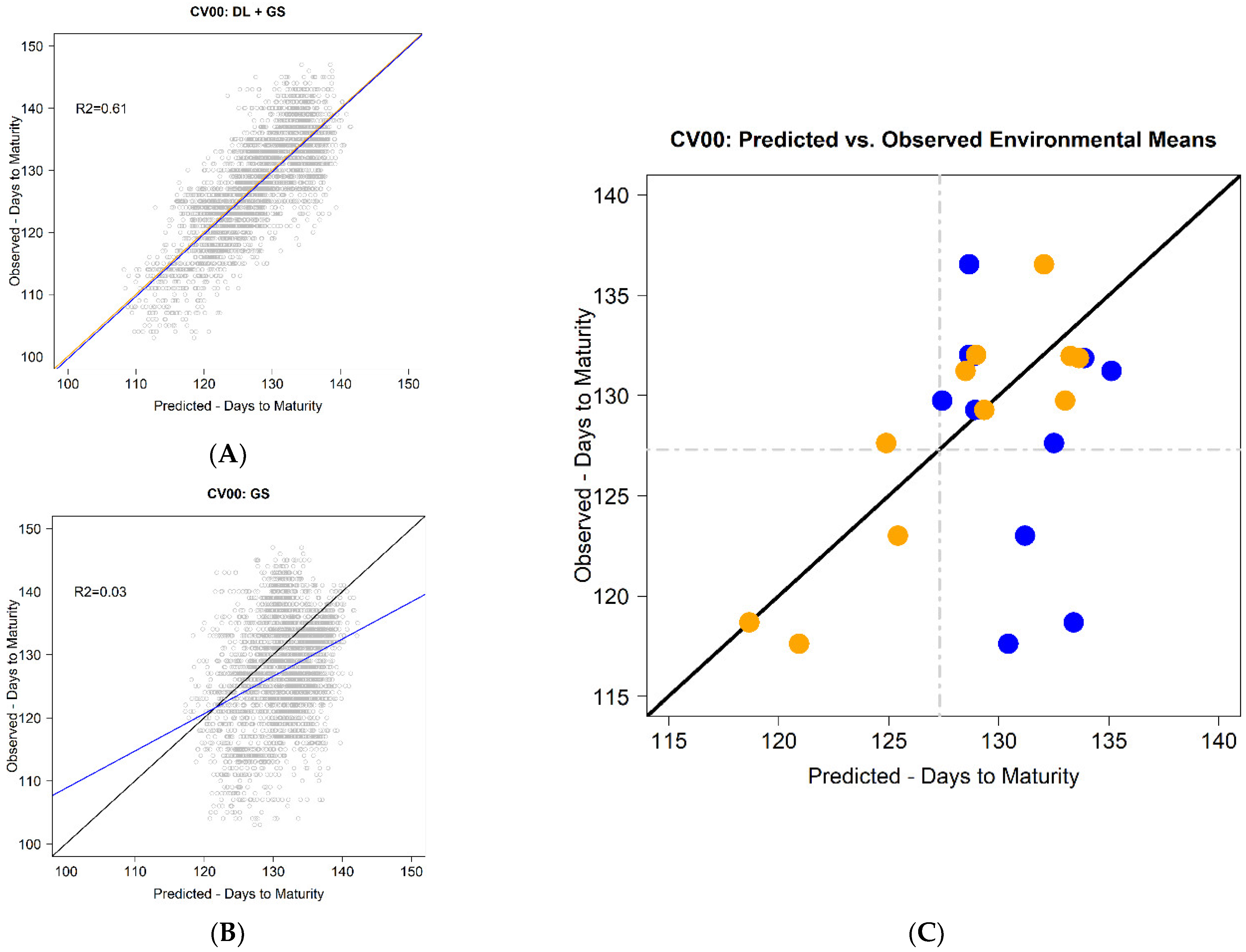
We considered two relevant scenarios that would likely be of interest to soybean breeders: cross-validation (CV0) for predicting tested genotypes in unobserved environments and CV00 for predicting untested genotypes in unobserved environments. In both cases, the testing set size varied between 127 and 367, depending on the environment to be predicted; furthermore, the training set size varied accordingly. In CV0, the cross-validation was realized by deleting the phenotypic data from all genotypes at the target environment; then, the genotypes observed in the remaining environments were used for model training in a leave-one-environment-out scheme. Thus, no randomization was involved when selecting the training and testing sets. For CV00, not only the phenotypic information of the testing environment was deleted as in the previous case but also the phenotypic information of the genotype of interest was deleted from all the environments in the training set. In this case, a validation scheme similar to the leave-one-observation-out scheme was adopted without considering any randomization process for composing testing and training sets.
2.4. Predicting Genotypic Phenotypes in Unobserved Environments
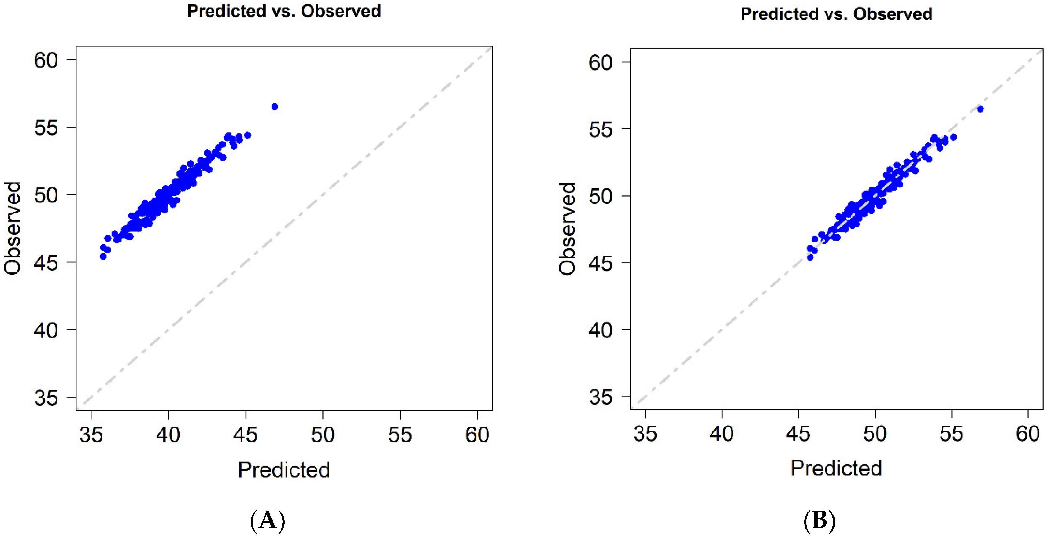
As mentioned before, GP can be a precise tool for generating rankings of the performance of genotypes in untested environments; however, in these cases, a large bias between predicted and observed values is expected.
Figure 1A exemplifies the case where a high correlation between predicted and observed values is obtained; however, it also shows a relatively large bias of the predicted values. A potential solution is to correct these predicted values using a constant, as depicted in
Figure 1B.
2.5. Statistical Models
The genomic best linear unbiased prediction model (GBLUP) is one of the most common prediction models used for estimating the genetic value of untested individuals. It uses dense molecular marker information to leverage the genomic relationships (kinship matrix) amongst related individuals. The principal objective of the kinship matrix is to describe genomic similarities between pairs of individuals via covariance structures [
35]. In addition, the GBLUP model is one of the most convenient implementations to manage large numbers of genomic covariates [
7,
36].
Consider that
represents the DTM of the
soybean genotype (
i = 1, 2, 3, …, 367) observed in the
environment (
j = 1, 2, 3, …, 11, corresponding to NE_2011, IL_2012, NE_2012, KS_2012, OHmain_2012, OHmc_2012, IA_2013, IL_2013, IN_2013, OHmain_2013, and OHmc_2013). Further, assume that
can be described as the sum of a constant effect plus environmental and genomic deviations and an error term, as follows:
The term
is defined as a constant effect (the overall mean) common to all soybean genotypes across the 11 environments; the
are independent and identically distributed (IID) outcomes from a normal distribution
that represents the effect of the
environment;
is the vector of genomic effects with
defined as the genomic relationship matrix, with
representing the standardized matrix (by columns) of
molecular markers (analogous to method 1 in [
36]); and
are IID outcomes from an
distribution representing the error term. The terms
and,
correspond to the associated variance components of the random effects.
2.6. Daylength + Marker Data
Since the GP method is expected to deliver a large bias when predicting the DTM in unobserved environments (
Figure 1), some of the features of the methodology proposed in [
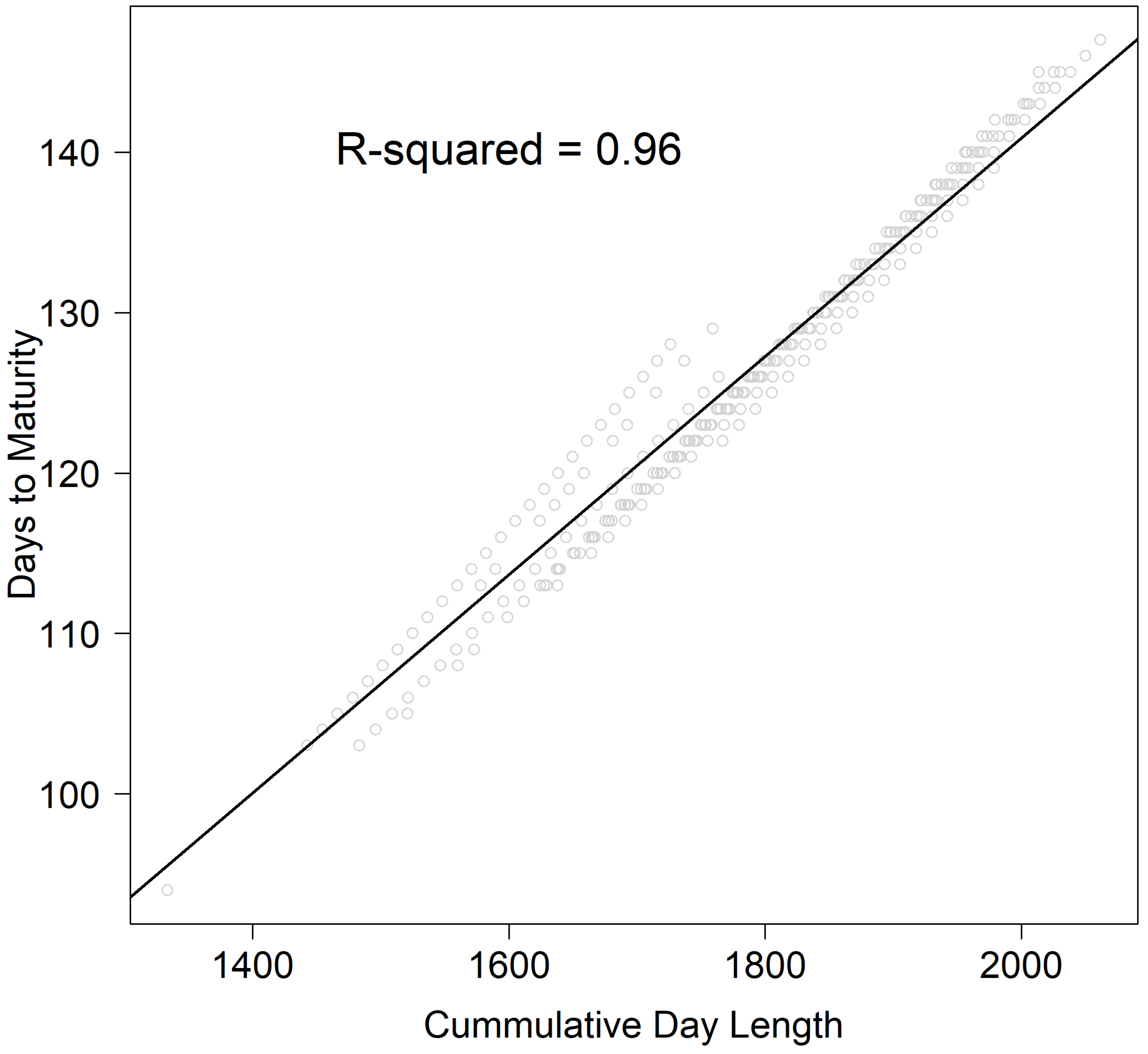
10] were adopted in our study. These authors proposed a novel method for predicting the rice phenological stage of days to heading in multiple populations. Their method allows for the use of daylength information in the prediction process by considering the daily progression of the daylight duration during the growing season. Because each genotype was already observed in several environments (11), numerical tendencies between the DTM and daylength can be detected by examining one genotype at a time. In this analysis, a clear trend relating to daylength at the R8 occurrence (
Figure 2) across environments was observed. As discussed in [
10], this gradient does not appear to be highly influenced by the initial daylength values at various planting dates across environments. However, it seems to be associated with the changing rate of the daylength starting at the planting date.
2.7. Concept in a Nutshell
To predict untested genotypes in unobserved environments, the first step was to estimate the potential DTM mean of the target environment. For this, the prediction of already tested genotypes (one at a time) in the unobserved environment (CV0) was performed. After predicting DTM for those genotypes in the training set, the next step was to obtain the expected DTM environmental mean by averaging the predicted values. Finally, for predicting DTM for the untested genotypes in the unobserved environment, the BLUPs derived from the traditional GP method were added to the estimated environmental mean. Further details of these methods are provided below.
2.8. C-Method
The C-method allows for the prediction of the DTM of tested genotypes in unobserved environments (CV0). For this, the daily daylength progression from the planting day to the DTM is needed. The first step was to characterize the daylength at the DTM (R8) time across environments. A third-degree polynomial equation was used to model the daylength as a function of the DTM:
where
represents the daylength at the DTM for the
ith genotype in the
jth environment as a function of time
t;
,
,
, and
are the model coefficients; and
is the error term and is assumed to be IID
in shape. In addition, the daylength for any environment can be obtained in advance just by knowing the location and planting date. The daily daylength progression of the unobserved environment was modeled with a third-degree polynomial equation as well:
where
represents the daylength of the target environment at the time
t;
,
,
. and
are the model coefficients; and
is the error term, which was assumed to be IID
in shape. The intersection point of these two curves provides an estimation of the DTM of the already tested genotype in the unobserved environment. To find the solution to these two equations, numerical evaluation was employed.
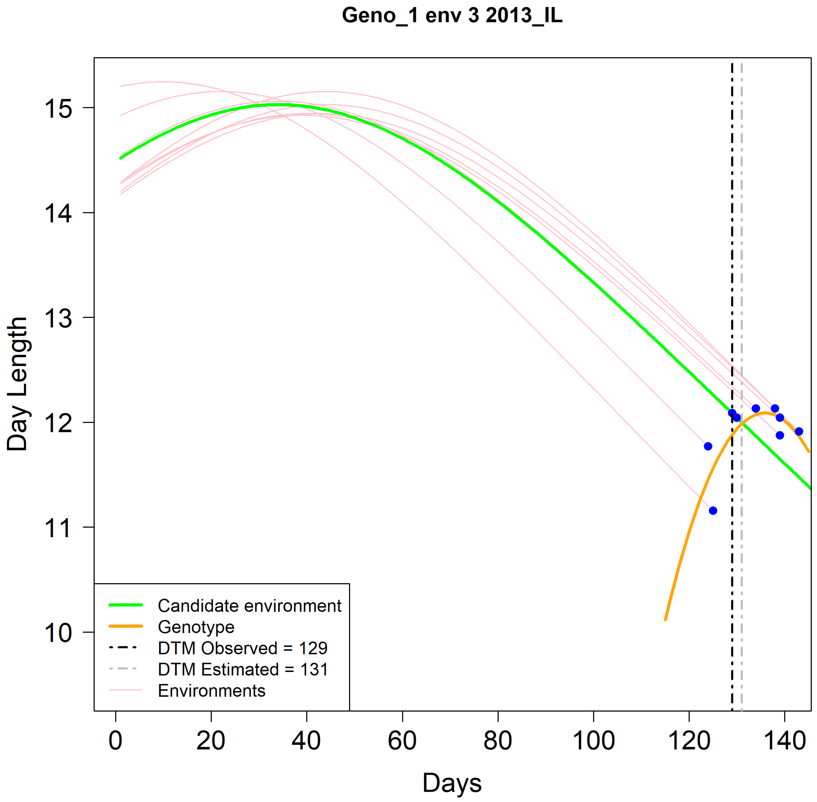
Figure 2 shows a graphical representation of the estimation of R8 using genotype Geno_1 in the Illinois environment IL_2013 as an example. In this case, the daylength progression (
y-axis) from planting until R8 (blue dots) is indicated with pink curves. The green line represents the daily daylength progression in the unobserved environment. The orange line is the fitted curve of the blue dots using the described third-degree polynomial equation. An estimation of the DTM was obtained by the crossing point of the green line with the orange line. In this example, the estimated DTM was 131 days, whereas the observed value was 129 days, which was indicative of a reasonable estimate. This procedure was repeated for each genotype in the training set, one at a time.
2.9. CB-Method
The main objective of our study consisted of predicting the DTM of untested genotypes in heretofore unobserved environments. Thus, compared with the previous method, an extra step was necessary. The potential environmental mean for the DTM in the unobserved target environment was estimated by computing the average of the predicted values that were obtained using the previously described C-method. Then, the next step consisted of obtaining the genomic BLUPs for the untested genotypes using the conventional GP model. Finally, the prediction of DTM for the untested genotype in the unobserved environment was found by adding the genomic BLUP of the ith untested genotype to the estimated environmental mean.
2.10. Demonstrative Example
For an easier understanding of how to implement the previous methods (C and CB) for predicting DTM of untested genotypes in unobserved environments, an example is provided. Let us assume there is phenotypic (DTM), genomic, and daylength information available for 100 genotypes observed in 10 environments conforming to the training set. Moreover, consider that we are interested in predicting the DTM for 5 untested genotypes (testing set) in an unobserved target environment from which we know the location and projected planting date.
The first step consists of estimating the environmental mean (DTM) in the target environment. For this, the C-method is implemented on each one of the 100 genotypes (one at a time) observed in other environments. Then, the environmental mean is calculated as the average of the 100 estimated DTM values. Once the environmental mean is estimated, the conventional GP model is implemented to compute the genomic BLUPs of those 5 genotypes in the testing set. The final step consists of adding to the BLUPs (5) the estimated environmental mean. In this case, the predicted DTM of the untested genotypes in the unobserved environment is a deviation (derived from the GP model) centered on the environmental mean.
2.11. Software
The statistical analyses were computed using R [
37]. The conventional GP model was fitted using the BGLR (Bayesian Generalized Linear Regression) R-package [
38], and the daylength information was obtained with the model proposed by [
34] included in the geosphere (v1.5–5) R package.
4. Discussion
In this study, genomic prediction was shown to be an efficient tool for predicting the ranking of complex traits (controlled by many genes of small effect) of untested genotypes in observed and unobserved environments [
7]. For example, using traits such as grain yield, disease, salinity, and drought tolerance, breeders focus the selection of the best genotypes occupying the desired tail of the distribution of the predicted GEBVs [
39]. When no information from the main environment is available for model calibration, GP might not be the most convenient method to implement when predicting a phenological stage, such as R8 in soybean. Among the potential disadvantages of using conventional GP models in the CV0 and CV00 scenarios, one may end up with a prediction of a developmental stage that is different from the one we are interested in due to a large bias between predicted and observed values. The C- and CB-methods, which are based on daylength information, helped to significantly reduce the bias without negatively affecting the predictive ability of the rankings.
The main purpose of this study was to develop and evaluate a method for predicting a time-related trait (here, the focus was on DTM) for untested soybean genotypes in unobserved environments. More specifically, we were interested in predicting the DTM; however, these developments can be extended to other important growing stages, such as days to flowering (R1) and R5. For this, a method was implemented that leveraged daylength information in the modeling process while considering two important prediction scenarios that are of interest to breeders. The first scenario (CV0) considered the prediction of already-tested genotypes in unobserved environments where a breeding line might be grown and have an adaptive fit. Two prediction strategies were implemented (the C-method and conventional GP). The second scenario (CV00) considered the prediction of untested genotypes in unobserved environments. In this case, two prediction strategies also were implemented (the CB-method and conventional GP).
The results obtained using the CV0 scheme were promising when using the C-method because it returned a smaller RMSE of 4.7 for DTM compared with the GP model (9.4). Moreover, the PODEM was significantly reduced under the C-method compared with the GP model from [−19.2, 11.9] days to [−3.4, 4.5] days. However, the average PC was slightly reduced from 0.805 to 0.768 with the C-method compared with the GP model. In general, the accuracy of the C-method outperformed the results from the conventional GP model. For example, RMSE was reduced by 50% (9.4 − 4.7 = 4.7), while the PODEM was reduced to one-quarter with the method that used daylength information.
These results were similar to those presented by Jarquin et al. [
10] who predicted days to heading in rice populations (112 genotypes tested in 51 environments) with the CV0 scheme. In their case, the C-method returned an RMSE of 3.9 days, with a PODEM that varied from −4.95 to 4.67 days and a PC of 0.98. In contrast, with the GP model, the corresponding values were an RMSE of 18.1 days, a PC of 0.41, and a PODEM that varied from −31.5 to 28.7 days. Chen [
40] performed a similar study by comparing the predictive accuracy of three approaches, namely, a crop growth model, a machine learning model, and a combination of these two models, for predicting days to heading in rice.
The authors considered genotypic information, environmental variables (daylength and daily temperature), and planting and headings dates of 112 cultivars/lines tested in seven locations over 14 years for a total of 64 environments. They obtained an RSME of 6.47 days when deleting one genotype from the rice data set. Our results were in line with these when using two foregoing rice studies [
10,
40], but closer to those from [
10]. One possible explanation might be that both traits in both crops responded similarly to daylength, coupled with the fact that we implemented almost the same methodology without taking into consideration the temperature or any other weather variable. It is worth noting that [
17] proposed a soybean model based on non-linear temperature and photoperiod data that was tested in a six-year soybean experiment.
These authors accomplished an RMSE of 1.8 days in a cultivar × sowing date experiment when predicting major reproductive stages in soybean (R1—first flower, R3—beginning pod, R5—beginning seed, and R7—physiological maturity). However, one of the disadvantages of their method is that the environmental conditions must be provided in advance or at least virtually (day-by-day). For example, the temperature is not constant over seasonal time and weather parameter data in any given year can deviate significantly from historical climatic normals, complicating the prediction process when prediction involves the use of crop models.
Regarding the most complex and interesting prediction scenario (CV00), the obtained results using the CB-method were clearly superior when compared with the GP model. It returned an RMSE of 5.2 days, whereas the RSME for GP was 7.8 days. The PODEM values varied from −3.3 to 4.4, but with the GP implementation, the respective values were −14.7 and 7.9 days, representing a reduction to one-third
using the CB-method. Notably, the average PC remained unaffected; it was 0.667, whereas the GP method returned 0.665. In [
10], when predicting days to heading in rice under the CV00 scenario (CB-method), the RMSE was 7.3 days, the PC was 0.93, and the PODEM varied from −6.4 to 4.1 days; in contrast, the conventional GP model returned an RMSE of 18.1 days, a PC of 0.41, and a PODEM that varied from −31.5 to 28.7 days. In the study performed by Chen et al. [
40] the integrated crop growth models and machine learning techniques, under the CV00 scheme (i.e., predicting untested genotypes in untested environments), the RMSE was 7.69 days. Their results are consistent with those from [
10] and the results obtained in our study.
Although the multiple E/e loci in soybean exert major phenotypic effects on flowering and maturity time [
26,
31], we did not consider these in our study. Their various allelic combinations provide a genetic basis for the adaptation of genotypes to certain latitudes and weather conditions [
22]. For instance, Doubler [
41] compared the prediction of using genome-wide markers and E genes associated with relative maturity (RM) in commercial soybean varieties. These authors determined allele effects in four prediction models: two models with traditional MAS (specific E gene and expanded E gene) and two GP models with different marker densities. The whole-genome marker GP and expanded E gene models returned the best results with average Pearson correlations of 0.93 and 0.94, respectively. For the E-gene-specific model, the prediction accuracy was slightly reduced to 0.8. These results provided insights into the potential of these major genes for predicting time-related traits; however, these authors did not consider predicting in unobserved environments, which could have led to a large bias.
Messina et al. [
42] designed a strategy by combining the ecophysiological model CROPGRO-Soybean with linear models for predicting growth parameters specific to each cultivar based on genetic E loci. These authors established an experiment in 2001 in Florida to collect data for model calibration, then used these values for predicting the days to the occurrence of various phenological stages of cultivars established in (
i) Florida (2002) and (
ii) Illinois for several location–year combinations. The root-mean-square error between the predicted and observed values of those genotypes grown in Florida were approximately 5 days, while for the Illinois variety trials, they were 7.5 days. Since then, more loci were detected and, at the same time, genomics has become more advanced. Given the potential yield-predictive ability of crop models, it is opportune to develop a genomic model for R8.
Recently, McCormick et al. [
43] proposed a strategy that leverages human-defined models of soybean phenology and data-driven machine learning models that accomplish accurate and interpretable predictions. These authors leveraged the knowledge-based models using machine learning techniques for predicting days to flowering (R1) and physiological maturity (R7), among other traits. For R1, the mean absolute error (MAE) was 4.41 days, while for the knowledge-based model, which was used as the benchmark, returned an MAE of 6.94 days. Regarding R7, the corresponding MAE was 5.27 days, while the knowledge-based model returned 15.53 days.
The C- and CB-methods showed that the use of daylength information in both prediction scenarios outperformed the prediction accuracy of conventional methods based on genome-wide markers, or in sets of major genes controlling this trait. The C-method takes advantage of phenotypic information of the same genotype observed in many other environments, whereas the CB-method uses the results of the C-method to predict untested genotypes in unobserved environments, thereby leveraging both phenotypic and molecular marker information, plus daylength information. The advantage of using these day-length-based methods is that theoretical values of daily daylength data can be obtained before observing cultivars in fields and the environmental conditions. These findings could help breeders to better plan their experiments when interested in phenology traits that are critical for the adaptive fit of breeding line selections that are destined to be released as new cultivars.


 ,
, 


