
Linking Management, Environment and Morphogenetic and Structural Components of a Sward for Simulating Tiller Density Dynamics in Bahiagrass (Paspalum notatum)

Abstract
:
1. Introduction
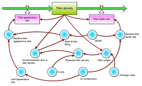
2. The Model


| Symbol | Description | Unit |
|---|---|---|
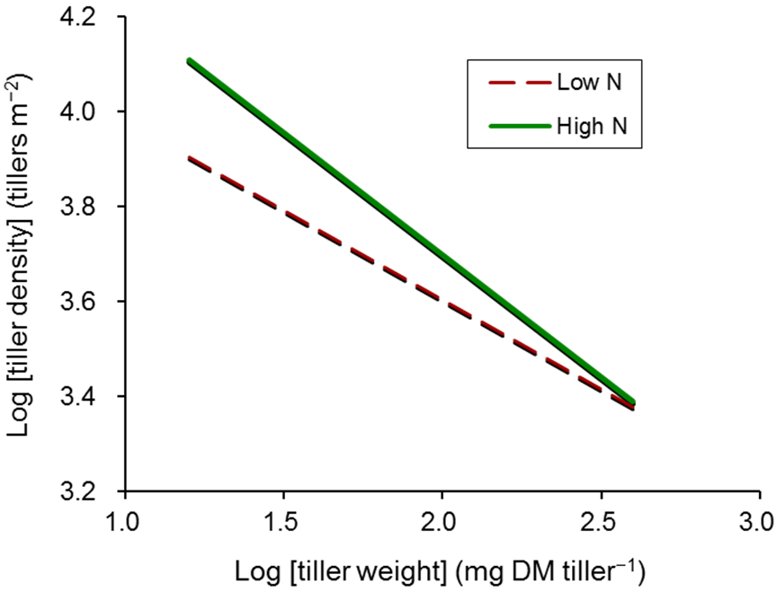
| Intercept of the standard relationship between tiller density and tiller weight | log tillers m−2 | |
| Slope of the standard relationship between tiller density and tiller weight | log tillers m−2 (log mg DM tiller−1)−1 | |
| Tiller density | tillers m−2 | |
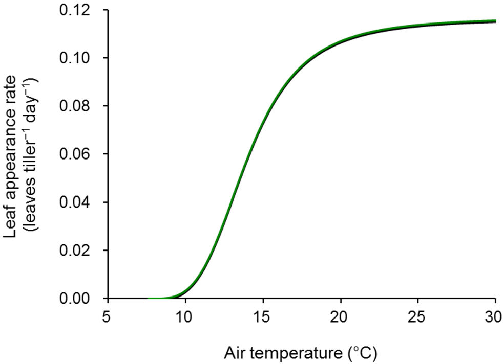
| Actual: expected ratio in tiller density | fraction | |
| Expected tiller density | tillers m−2 | |
| Annual nitrogen fertilizer rate | g m−2 year−1 | |
| Rate of site filling | tillers leaf−1 | |
| Herbage mass | g DM m−2 | |
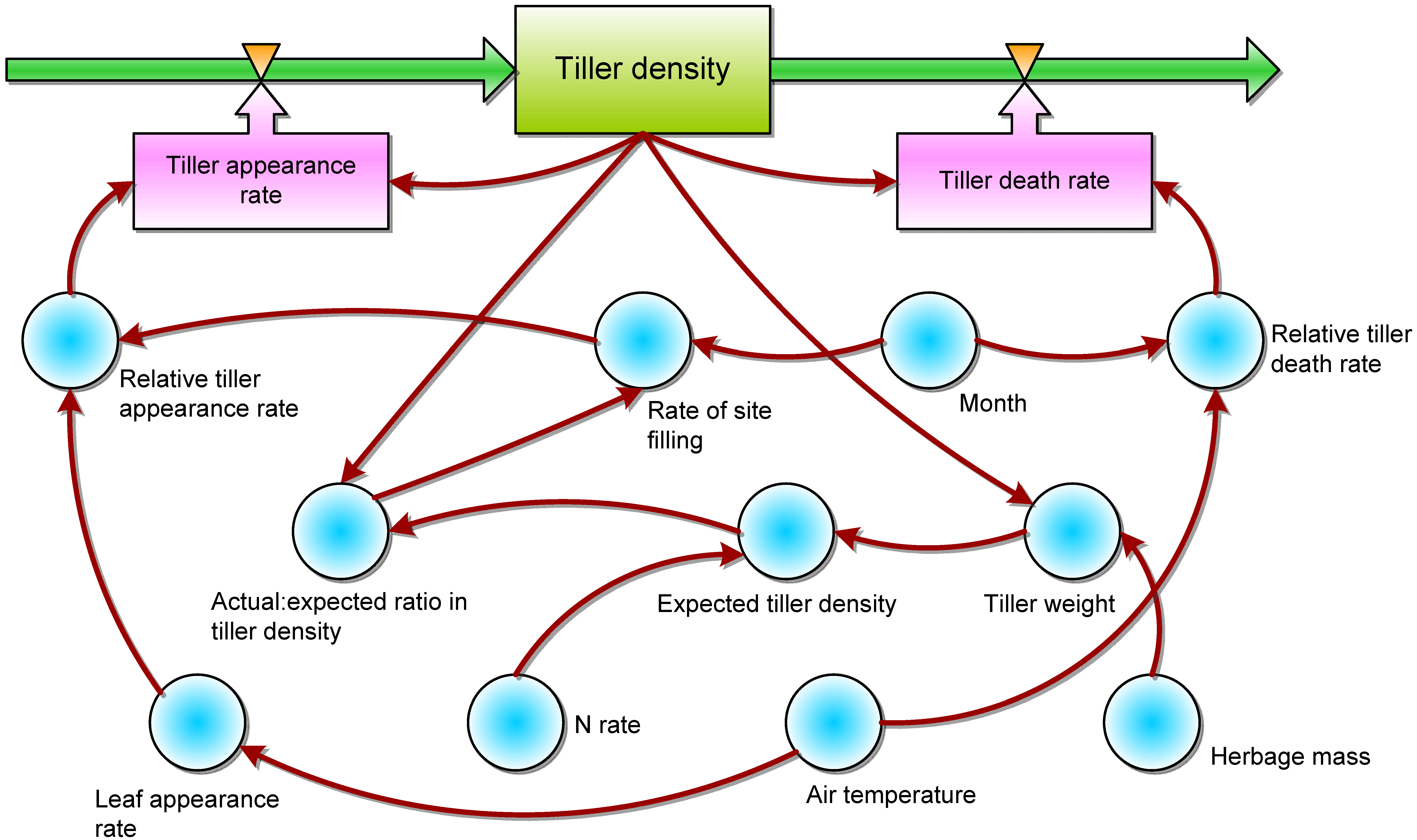
| Leaf appearance rate | leaves tiller−1 day−1 | |
| Tiller appearance rate | tillers m−2 day−1 | |
| Relative tiller appearance rate | tillers tiller−1 day−1 | |
| Tiller death rate | tillers m−2 day−1 | |
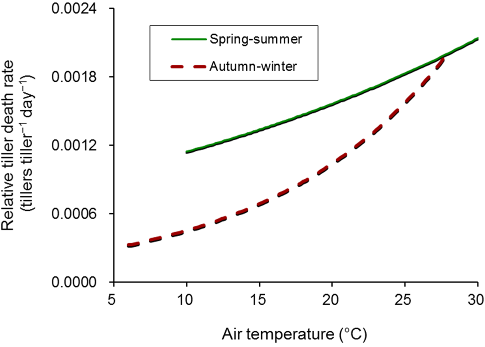
| Relative tiller death rate | tillers tiller−1 day−1 | |
| Time | day | |
| Mean daily air temperature | °C | |
| Tiller weight | mg DM tiller−1 |
2.1. Rate of Change in Tiller Density
2.2. Tiller Appearance


2.3. Tiller Death

3. Model Performance
3.1. Calibration

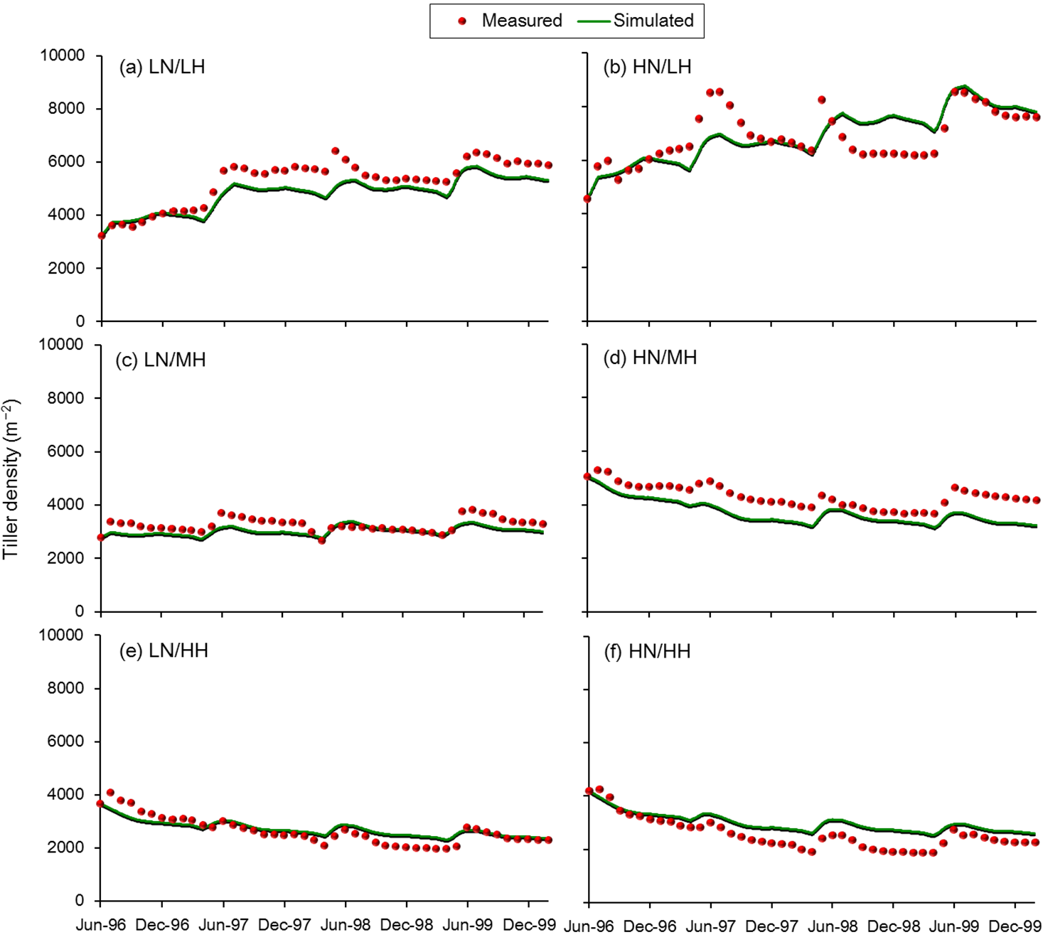
3.2. Validation
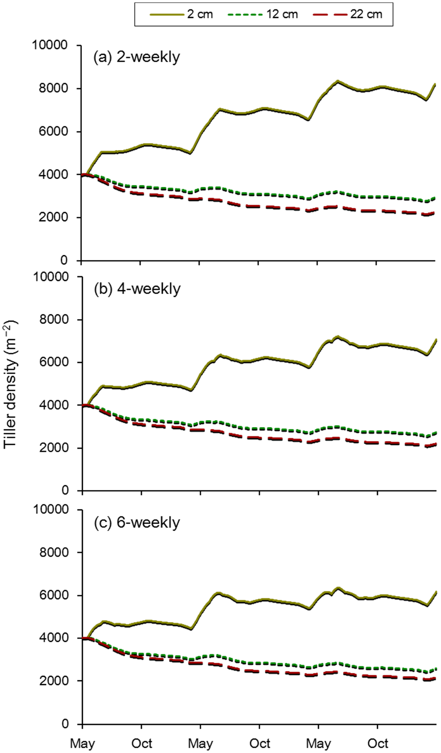
4. Use of the Model


5. Discussion
Acknowledgments
Conflicts of Interest
References
- Chapman, D.F.; Lemaire, G. Morphogenetic and structural determinants of plant regrowth after defoliation. In Proceedings of the XVII International Grassland Congress, Palmerston North, Hamilton, Lincoln and Rockhampton, New Zealand and Australia, 8–21 February 1993; pp. 95–104.
- Lemaire, G.; Chapman, D. Tissue flows in grazed plant communities. In The Ecology and Management of Grazing Systems; Hodgson, J., Illius, A.W., Eds.; CAB International: Wallingford, UK, 1996; pp. 3–36. [Google Scholar]
- Matthew, C.; Agnusdei, M.G.; Assuero, S.G.; Sbrissia, A.F.; Scheneiter, O.; da Silva, S.C. State of knowledge in tiller dynamics. In Proceedings of the 22nd International Grassland Congress, Sydney, Australia, 15–19 September 2013; New South Wales Department of Primary Industry: Orange, New South Wales, Australia, 2013; pp. 1041–1044. [Google Scholar]
- Skerman, P.J.; Riveros, F. Tropical Grasses; FAO: Rome, Italy, 1989; pp. 571–575. [Google Scholar]
- Hirata, M.; Ogawa, Y.; Koyama, N.; Shindo, K.; Sugimoto, Y.; Higashiyama, M.; Ogura, S.; Fukuyama, K. Productivity of bahiagrass pastures in south-western Japan: Synthesis of data from grazing trials. J. Agron. Crop Sci. 2006, 192, 79–91. [Google Scholar] [CrossRef]
- Beaty, E.R.; Brown, R.H.; Morris, J.B. Response of Pensacola bahiagrass to intense clipping. In Proceedings of the XI International Grassland Congress, Surfers Paradise, Australia, 13–23 April 1970; University of Queensland Press: St. Lucia, Queensland, Australia, 1970; pp. 538–542. [Google Scholar]
- Beaty, E.R.; Engel, J.L.; Powell, J.D. Yield, leaf growth, and tillering in bahiagrass by N rate and season. Agron. J. 1977, 69, 308–311. [Google Scholar] [CrossRef]
- Stanley, R.L.; Beaty, E.R.; Powell, J.D. Forage yield and percent cell wall constituents of Pensacola bahiagrass as related to N fertilization and clipping height. Agron. J. 1977, 69, 501–504. [Google Scholar] [CrossRef]
- Hirata, M.; Ueno, M. Response of bahiagrass (Paspalum notatum Flügge) sward to cutting height. 1. Dry weight of plant and litter. J. Jpn. Grassl. Sci. 1993, 38, 487–497. [Google Scholar]
- Hirata, M. Response of bahiagrass (Paspalum notatum Flügge) sward to cutting height. 3. Density of tillers, stolons and primary roots. J. Jpn. Grassl. Sci. 1993, 39, 196–205. [Google Scholar]
- Hirata, M. Response of bahiagrass (Paspalum notatum Flügge) sward to nitrogen fertilization rate and cutting interval. 1. Dry weight of plant and litter. J. Jpn. Grassl. Sci. 1994, 40, 313–324. [Google Scholar]
- Pakiding, W.; Hirata, M. Tillering in a bahia grass (Paspalum notatum) pasture under cattle grazing: Results from the first two years. Trop. Grassl. 1999, 33, 170–176. [Google Scholar]
- Hirata, M. Effects of nitrogen fertiliser rate and cutting height on leaf appearance and extension in bahia grass (Paspalum notatum) swards. Trop. Grassl. 2000, 34, 7–13. [Google Scholar]
- Pakiding, W.; Hirata, M. Leaf appearance, death and detachment in a bahia grass (Paspalum notatum) pasture under cattle grazing. Trop. Grassl. 2001, 35, 114–123. [Google Scholar]
- Hirata, M.; Pakiding, W. Tiller dynamics in a bahia grass (Paspalum notatum) pasture under cattle grazing. Trop. Grassl. 2001, 35, 151–160. [Google Scholar]
- Hirata, M.; Pakiding, W. Dynamics in tiller weight and its association with herbage mass and tiller density in a bahia grass (Paspalum notatum) pasture under cattle grazing. Trop. Grassl. 2002, 36, 24–32. [Google Scholar]
- Hirata, M.; Pakiding, W. Dynamics in lamina size in a bahia grass (Paspalum notatum) pasture under cattle grazing. Trop. Grassl. 2002, 36, 180–192. [Google Scholar]
- Pakiding, W.; Hirata, M. Effects of nitrogen fertilizer rate and cutting height on tiller and leaf dynamics in bahiagrass (Paspalum notatum Flügge) swards: Tiller appearance and death. Grassl. Sci. 2003, 49, 193–202. [Google Scholar]
- Pakiding, W.; Hirata, M. Effects of nitrogen fertilizer rate and cutting height on tiller and leaf dynamics in bahiagrass (Paspalum notatum Flügge) swards: Leaf appearance, death and detachment. Grassl. Sci. 2003, 49, 203–210. [Google Scholar]
- Pakiding, W.; Hirata, M. Effects of nitrogen fertilizer rate and cutting height on tiller and leaf dynamics in bahiagrass (Paspalum notatum Flügge) swards: Leaf extension and mature leaf size. Grassl. Sci. 2003, 49, 211–216. [Google Scholar]
- Hirata, M.; Pakiding, W. Tiller dynamics in bahia grass (Paspalum notatum): An analysis of responses to nitrogen fertiliser rate, defoliation intensity and season. Trop. Grassl. 2004, 38, 100–111. [Google Scholar]
- Hirata, M. Canopy dynamics in bahia grass (Paspalum notatum) swards. In Recent Research Developments in Crop Science; Pandalai, S.G., Ed.; Research Signpost: Kerala, India, 2004; Volume 1, pp. 117–145. [Google Scholar]
- Hirata, M. Modelling tiller density dynamics in a grass sward. In XX International Grassland Congress: Offered Papers; O’Mara, F.P., Wilkins, R.J., t’Mannetje, L., Lovett, D.K., Rogers, P.A.M., Boland, T.M., Eds.; Wageningen Academic Publishers: Wageningen, The Netherlands, 2005; p. 870. [Google Scholar]
- Davies, A. Leaf tissue remaining after cutting and regrowth in perennial ryegrass. J. Agric. Sci. Camb. 1974, 82, 165–172. [Google Scholar] [CrossRef]
- Thomas, H. Terminology and definitions in studies of grassland plants. Grass Forage Sci. 1980, 35, 13–23. [Google Scholar] [CrossRef]
- Yoda, K.; Kira, T.; Ogawa, H.; Hozumi, K. Intraspecific competition among higher plants. XI. Self-thinning in overcrowded pure stands under cultivated and natural conditions. J. Biol. Osaka City Univ. 1963, 14, 107–129. [Google Scholar]
- Hirata, M. Quantifying spatial heterogeneity in herbage mass and consumption in pastures. J. Range Manag. 2000, 53, 315–321. [Google Scholar] [CrossRef]
- Hirata, M. Estimating herbage and leaf utilization in bahiagrass (Paspalum notatum Flügge) swards from height measurements. Grassl. Sci. 2002, 48, 105–109. [Google Scholar]
- Korte, C.J. Tillering in ‘Grasslands Nui’ perennial ryegrass swards. 2. Seasonal pattern of tillering and age of flowering tillers with two mowing frequencies. N. Z. J. Agric. Res. 1986, 29, 629–638. [Google Scholar] [CrossRef]
- Bullock, J.M.; Hill, B.C.; Silvertown, J. Tiller dynamics of two grasses—Response to grazing, density and weather. J. Ecol. 1994, 82, 331–340. [Google Scholar] [CrossRef]
- Sbrissia, A.F.; da Silva, S.C.; Sarmento, D.O.L.; Molan, L.K.; Andrade, F.M.E.; Gonçalves, A.C.; Lupinacci, A.V. Tillering dynamics in palisadegrass swards continuously stocked by cattle. Plant Ecol. 2010, 206, 349–359. [Google Scholar] [CrossRef]
- Dayan, E.; van Keulen, H.; Dovrat, A. Tiller dynamics and growth of Rhodes grass after defoliation: A model named TILDYN. Agro-Ecosystems 1981, 7, 101–112. [Google Scholar] [CrossRef]
- Coughenour, M.B.; McNaughton, S.J.; Wallace, L.L. Simulation study of East-African perennial graminoid responses to defoliation. Ecol. Model. 1984, 26, 177–201. [Google Scholar] [CrossRef]
- Schapendonk, A.H.C.M.; Stol, W.; van Kraalingen, D.W.G.; Bouman, B.A.M. LINGRA, a sink/source model to simulate grassland productivity in Europe. Eur. J. Agron. 1998, 9, 87–100. [Google Scholar] [CrossRef]
- Soussana, J.F.; Oliveira Machado, A. Modelling the dynamics of temperate grasses and legumes in cut mixtures. In Grassland Ecophysiology and Grazing Ecology; Lemaire, G., Hodgson, J., de Moraes, A., de F. Carvalho, P.C., Nabinger, C., Eds.; CABI Publishing: Wallingford, UK, 2000; pp. 169–190. [Google Scholar]
© 2015 by the authors; licensee MDPI, Basel, Switzerland. This article is an open access article distributed under the terms and conditions of the Creative Commons Attribution license (http://creativecommons.org/licenses/by/4.0/).
Share and Cite
Hirata, M. Linking Management, Environment and Morphogenetic and Structural Components of a Sward for Simulating Tiller Density Dynamics in Bahiagrass (Paspalum notatum). Agriculture 2015, 5, 330-343. https://0-doi-org.brum.beds.ac.uk/10.3390/agriculture5020330
Hirata M. Linking Management, Environment and Morphogenetic and Structural Components of a Sward for Simulating Tiller Density Dynamics in Bahiagrass (Paspalum notatum). Agriculture. 2015; 5(2):330-343. https://0-doi-org.brum.beds.ac.uk/10.3390/agriculture5020330
Chicago/Turabian StyleHirata, Masahiko. 2015. "Linking Management, Environment and Morphogenetic and Structural Components of a Sward for Simulating Tiller Density Dynamics in Bahiagrass (Paspalum notatum)" Agriculture 5, no. 2: 330-343. https://0-doi-org.brum.beds.ac.uk/10.3390/agriculture5020330